Sage Journals: Discover world-class research

Abstract

A new slip-line field model and its associated hodograph of rounded-edge cutting tool were developed for orthogonal micro-cutting operation using matrix technique. The new model considers the existence of dead metal zone in front of the rounded-edge cutting tool. The ploughing forces, chip up-curl radii, chip thicknesses, primary shear zone thicknesses and lengths of bottom side of the dead metal zone are obtained by solving the model depending on the experimental resultant force data. The effects of cutting edge radius, uncut chip thickness, cutting speed and rake angle on these outputs are specified.

Keywords

Slip-line field model rounded-edge cutting tool dead metal zone ploughing force micro-machining

Introduction

The effects of cutting edge geometry should be known to understand the precision of micro- and nano-machining operations. In the previous works of Merchant,¹ Lee and Shaffer² and Oxley³, the cutting tool edge was assumed to be perfectly sharp to simplify the modelling of metal cutting. Besides, Maity and Das^4–7 carried out theoretical slip-line field solutions of perfectly sharp cutting tool for orthogonal metal cutting, and researchers considered that the sticking and slipping contact occurred at the chip–tool interface. Fang et al.⁸ developed a universal slip-line model of two-dimensional (2D) machining for restricted perfectly sharp cutting tools, and the developed model provided the effects of the chip up-curling and the chip back-flow. Fang^9,10 presented a slip-line model for a perfectly sharp cutting tool, and this model considered the tool–chip contact on the tool secondary rake face. The forces, chip thickness and tool–chip contact length can be determined using the proposed slip-line model. Das et al.¹¹ proposed a slip-line field model for perfectly sharp cutting tools which accepts the adhesion friction at the chip–tool interface by using Kudo’s¹² basic slip-line field. Fang and Dewhurst¹³ developed a slip-line model for perfectly sharp cutting tools with built-up edge formation. The model predicted the length and height of the built-up edge, cutting and thrust forces, chip up-curl radius, chip thickness and tool–chip contact length. Das and Dundur¹⁴ developed slip-line field solutions for metal cutting with perfectly sharp tools. Ye et al.¹⁵ presented a slip-line model for perfectly sharp tool of pressure-sensitive material and examined the effect of the material pressure sensitivity on the cutting operation.

However, Albrecht¹⁶ reported that a perfectly sharp cutting tool edge cannot be produced, and the nature radius of the cutting edge was determined to be 0.007 mm. Therefore, various slip-line analyses were carried out using the rounded-edge cutting tools. Abdelmoneim and Scrutton¹⁷ and Abdelmoneim¹⁸ developed a slip-line model for rounded-edge cutting tools, and this model considered the effects of dead metal zone in mathematical formulation. Waldorf et al.¹⁹ presented a slip-line model of the ploughing process for rounded-edge cutting tool in orthogonal machining. The model was based on the assumption of a dead metal zone in front of the finite radius of cutting edge. Fang^20,21 proposed a slip-line model to analyse orthogonal metal cutting with a rounded-edge cutting tool. According to the researcher, the tool edge roundness was defined by the tool edge radius, position of the stagnation point and tool–chip frictional shear stress. Fang and Fang²² investigated the finish cutting with a rounded-edge tool by both theoretical and experimental studies. The two models, including an analytical model and a finite element (FE) model, considered the effects of strain, strain rate, cutting tool edge radius and temperature on the material flow stress. Wang and Jawahir²³ developed a slip-line model for rounded-edge cutting tool–restricted contact grooved tools. Karpat and Ozel²⁴ presented the cutting mechanics with curvilinear edge cutting tool in the presence of dead metal zone to determine the effects of edge geometry and cutting conditions on the friction and the cutting tool temperature. An analytical slip-line field model was performed to investigate the cutting mechanics and friction at the tool–chip and tool–workpiece interfaces. Jin and Altintas²⁵ developed a slip-line field model for the micro-cutting process with a rounded-edge cutting tool. Uysal et al.²⁶ presented a slip-line model of the rounded-edge tool for metal cutting. The model considered the existence of a dead metal zone and consisted of seven sub-regions. Ozturk and Altan²⁷ presented a slip-line model for a rounded-edge tool. The model was divided into eight sub-regions, and the slip-line angles were calculated depending on the experimental force data. Ozturk et al.²⁸ metallographically analysed the dead metal zone during metal cutting with the rounded-edge cutting tool. Ozturk and Altan²⁹ experimentally investigated the effect of the separation point on metal flows and the material behaviour in front of the tool face with a rounded-edge cutting tool.

In the Fang’s^20,21 and Wang and Jawahir’s²³ studies, the rounded-edge cutting tool was divided into two straight chords to simplify the models, and the existence of a dead metal zone was neglected. In previous studies, some researchers assumed the cutting tool as perfectly sharp, and some researchers neglected the dead metal zone. It is known that the cutting tools have a little cutting edge radius, and in some cases, they are specially produced with a large cutting edge radius. This cutting edge radius causes the dead metal zone.

In this study, a new slip-line field model and its associated hodograph were developed for a rounded-edge cutting tool by considering the dead metal zone formation. The mathematical formulation of the new model was determined by employing the Dewhurst and Collins’³⁰ matrix technique.

The new slip-line field model

The new slip-line model for orthogonal cutting with a rounded-edge cutting tool was developed by assuming a dead metal zone formation. The new slip-line model and its hodograph can be seen in Figures 1 and 2, respectively, and this model has a dead metal zone (GSN) in front of rounded-edge cutting tool. The new slip-line model consists of eight slip-line angles (θ ₁, θ ₂, η ₁, η ₂, δ, δ ₂, δ ₃ and ψ) and two angles of vertices (α ₁ and α ₂). The angle α ₁ is between the free surface of workpiece and the straight A₃A₂ slip-line, and the angle α₂ is between the free surface of chip and the curved IA slip-line. Besides, the new model includes the angle δ ₁ between the straight AA₃ boundary and the cutting speed. If the slip-line angle ψ = 0, the region SCIJD disappears, and if the slip-line angle δ = 0, the region GKL disappears. In Figure 1, point S is called as separation point, and material flows upwards or downwards from point S.

Figure 1.

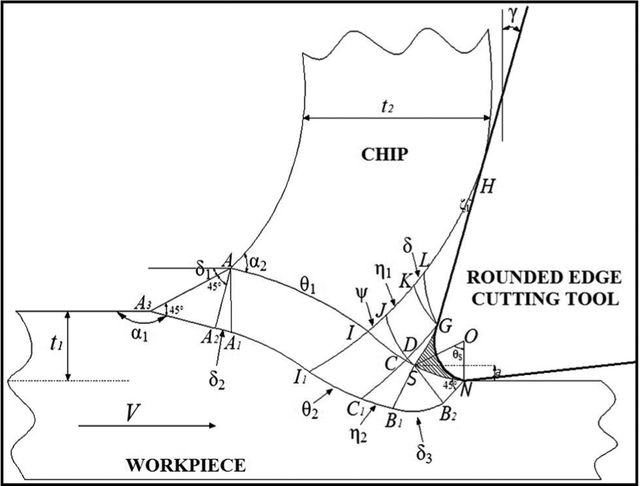
The new slip-line model for a rounded-edge cutting tool.

Figure 2.

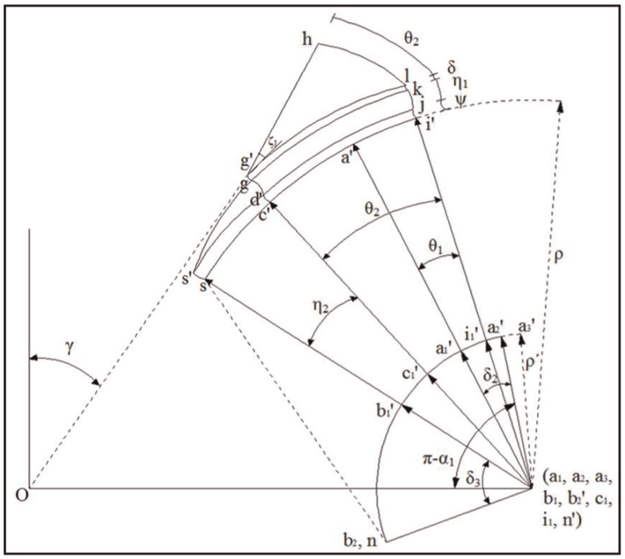
Hodograph of the new slip-line model.

The new slip-line model follows two traditional slip-line theory assumptions. The first is that the material deformation is under plane-strain conditions. For this reason, the new model is suitable for orthogonal metal cutting with continuous chip formation. The other assumption is that the workpiece material is rigid-plastic. In addition, it is accepted that the static forces are stable in the slip-line field.

Chip formation consists of the primary, secondary and tertiary shear zones; three transition regions; a material pre-flow region and a dead metal zone, as seen in Figure 3. The metal cutting models usually neglect the existence of these transition regions and the dead metal zone, but the shapes, sizes and locations of these transition regions and the dead metal zone depend on cutting conditions, tool geometries and workpiece materials.

Figure 3.

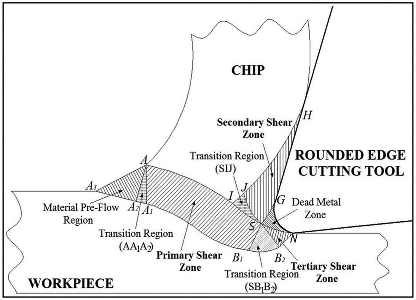
Shear zones and regions of the new slip-line model.

All 14 slip-line sub-regions of the new slip-line model of rounded-edge cutting tool for orthogonal machining are shown in Figure 4. Sub-region 1 is a non-uniform field with a straight boundary and formed by tool–chip friction on the tool rake face. In sub-region 1, the material flows from point G to point H and the tool–chip contact length is defined. Sub-region 6 is called as dead metal zone, and it occurs in front of the rounded-edge cutting tool. In sub-region 6, the material does not flow. The non-uniform sub-regions 2, 3 and 4 connect sub-regions 1 and 6. The non-uniform sub-regions 5 and 7 indicate the transition between the primary and secondary shear zones. Sub-region 8 is the tertiary shear zone. The non-uniform sub-region 9 defines the transition between the primary and secondary shear zones. The non-uniform sub-regions 10 and 11 represent the interaction between the primary and secondary shear zones. The non-uniform sub-region 12 provides the chip up-curling effect. The non-uniform sub-region 13 specifies the transition between the primary shear zone and the material pre-flow region, and the uniform sub-region 14 is formed from material pre-flow effect (Figure 4).

Figure 4.

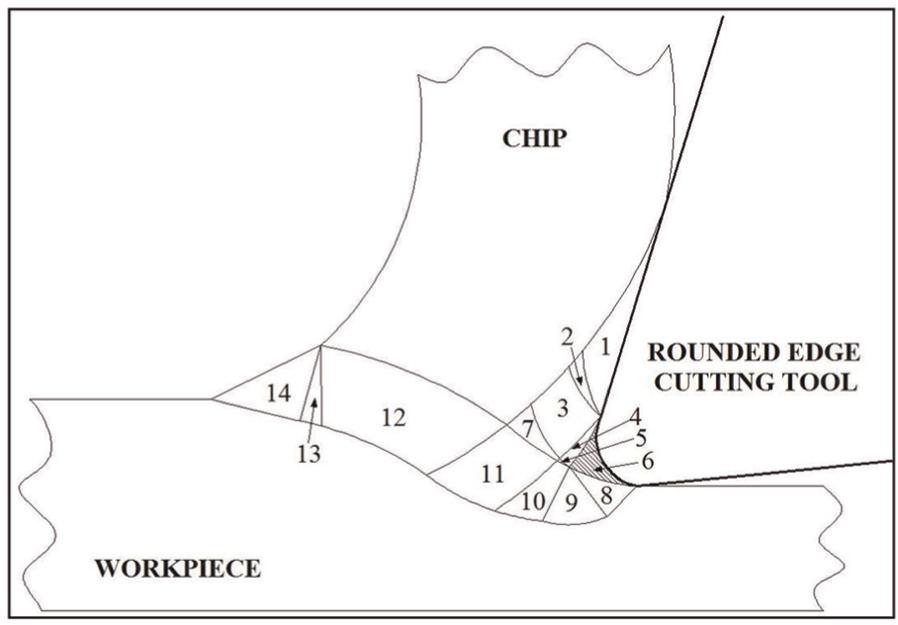
Slip-line sub-regions of the new slip-line model.

The new slip-line field model considers the cutting edge radius and the dead metal zone, and this model is adapted for cutting tools used in machining operations because perfectly sharp cutting tools cannot be produced and they have a little cutting edge radius. In some cases, cutting tools are specially produced with a large cutting edge radius. This cutting edge radius causes the dead metal zone. In most of the classic models, the chip formation occurs on a single shear plane. In the presented model, the chip deformation occurred in a shear zone differently from the classic models. This approach is much closer to practical metal cutting operations than a shear plane model. The new model considers the chip up-curling effect caused by the convex IA slip-line and the material pre-flow effect (slip-line sub-region AA ₂ A ₃, Figure 3) in the shear zone in contrast to the previous models. The new model clearly presents a strong interaction between the primary and secondary shear zones. As an example, a change in the slip-line sub-regions 1–5 and 7 in the secondary shear zone causes a change in the slip-line sub-regions 10 and 11 in the primary shear zone (Figure 4).

Mathematical formulation of the new slip-line field model

The matrix technique developed by Dewhurst and Collins³⁰ has been employed for numerically solving the mathematical formulation of the new slip-line model. This technique was expressed in Appendix 3. Also, Fang’s^20,21 work has been used to establish and solve the new slip-line field model.

Determination of the tool–chip friction

The tool–chip friction occurs on the tool rake face and is determined according to equation (1)²⁰

ζ = \frac{1}{2} {Cos}^{- 1} (τ / k)

(1)

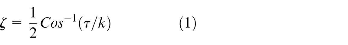
where ζ is the factor for tool–chip friction on the tool rake face, τ is the corresponding tool–chip frictional shear stress and k is the material shear flow stress.

Determination of the slip-lines in the secondary shear zone

The slip-lines HL and KJ seen in Figure 1 are two base slip-lines, and their radii are indicated as column vectors σ ₁ and σ ₂, respectively. In the following equations, P, P*, Q, Q*, R and G are the basic matrix operators defined by Dewhurst and Collins.³⁰ The angles θ ₁, θ ₂, δ, δ ₂, δ ₃, ψ, η ₁ and η ₂ shown in Figure 1 are slip-line angles.

Relationships among the slip-lines in the proposed new slip-line model

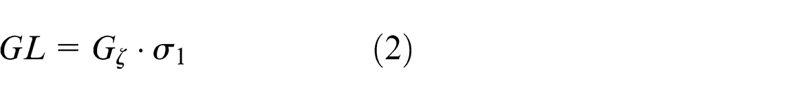
In the HLG slip-line region, GL is calculated as

GL = G_{ζ} \cdot σ_{1}

(2)

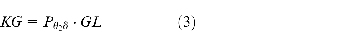
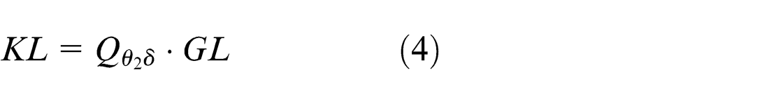
In the LKG slip-line region, KG and KL are given by

KG = P_{θ_{2} δ} \cdot GL

(3)

KL = Q_{θ_{2} δ} \cdot GL

(4)

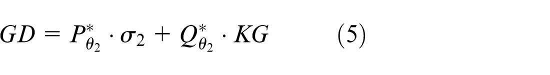
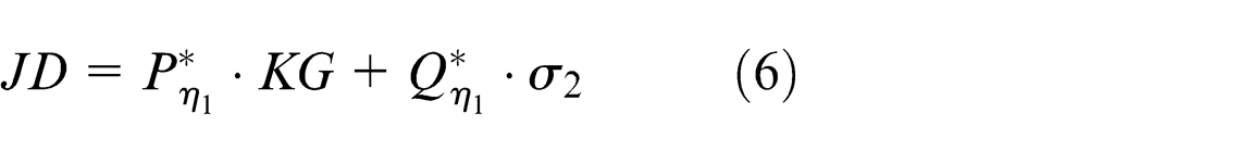
In the KJDG slip-line region, GD and JD are expressed as

GD = P_{θ_{2}}^{*} \cdot σ_{2} + Q_{θ_{2}}^{*} \cdot KG

(5)

JD = P_{η_{1}}^{*} \cdot KG + Q_{η_{1}}^{*} \cdot σ_{2}

(6)

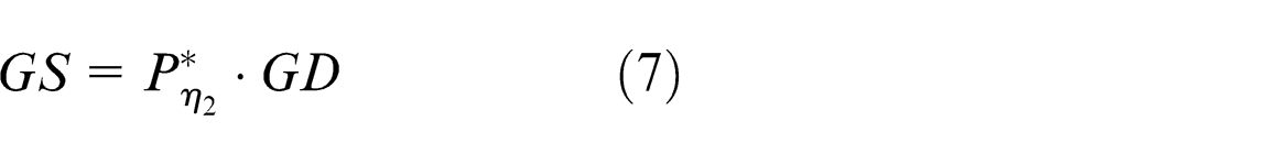
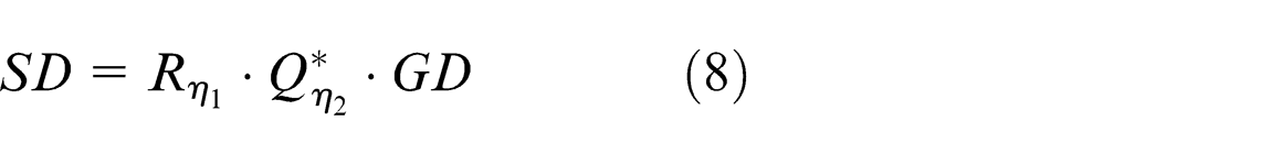
In the GDS slip-line region, GS and SD are represented by

GS = P_{η_{2}}^{*} \cdot GD

(7)

SD = R_{η_{1}} \cdot Q_{η_{2}}^{*} \cdot GD

(8)

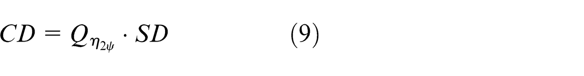
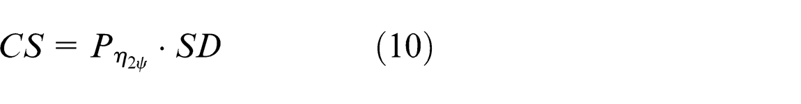
In the DCS slip-line region, CD and CS are calculated as

CD = Q_{η_{2 ψ}} \cdot SD

(9)

CS = P_{η_{2 ψ}} \cdot SD

(10)

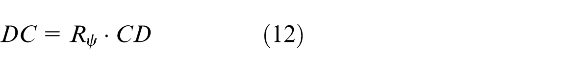
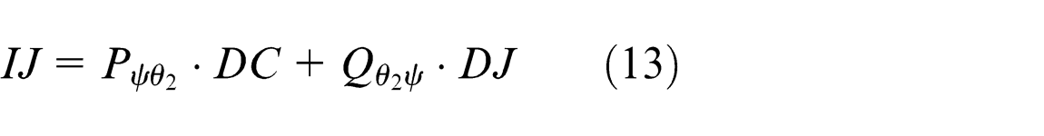
In the JICD slip-line region, DJ, DC, IJ and IC are determined by

DJ = R_{θ_{2}} \cdot JD

(11)

DC = R_{ψ} \cdot CD

(12)

IJ = P_{ψ θ_{2}} \cdot DC + Q_{θ_{2} ψ} \cdot DJ

(13)

IC = P_{θ_{2} ψ} \cdot DC + Q_{ψ θ_{2}} \cdot DJ

(14)

The convex IA slip-line is calculated by

IA = (ρ / ω) \cdot c

(15)

where ρ is the magnitude of total velocity jump across the slip-lines AICSN, ω is the angular velocity of a curled chip rotation and c is a column vector representing a unit circle as given in equation (16)

c = [\begin{matrix} \begin{matrix} 1 \\ 0 \\ 0 \end{matrix} \\ ⋮ \end{matrix}]

(16)

Relationships among the slip-lines in the hodograph of the proposed new slip-line model

Equations (17)–(22) are determined by Green³¹

i' c' = ρ \cdot c

(17)

i' a' = ω \cdot IA

(18)

i' j = ω \cdot IJ

(19)

kj = ω \cdot σ_{2}

(20)

kl = ω \cdot KL

(21)

hl = ω \cdot σ_{1}

(22)

In the i′jd′c′ slip-line region, jd′ and c′d′ are represented by

jd' = P_{ψ}^{*} . i' c' + Q_{ψ}^{*} . i' j

(23)

c' d' = P_{θ_{2}}^{*} \cdot i' j + Q_{θ_{2}}^{*} \cdot i' c'

(24)

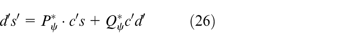
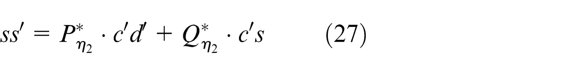
In the c′d′s′s slip-line region, c′s, d′s′ and ss′ are determined by

c' s = ρ \cdot c

(25)

d' s' = P_{ψ}^{*} \cdot c' s + Q_{ψ}^{*} c' d'

(26)

ss' = P_{η_{2}}^{*} \cdot c' d' + Q_{η_{2}}^{*} \cdot c' s

(27)

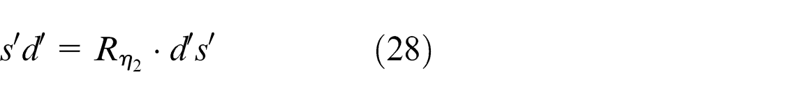
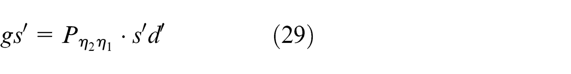
In the d′gs′ slip-line region, s′d′, gs′ and gd′ are calculated as

s' d' = R_{η_{2}} \cdot d' s'

(28)

gs' = P_{η_{2} η_{1}} \cdot s' d'

(29)

gd' = Q_{η_{2} η_{1}} \cdot s' d'

(30)

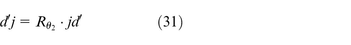
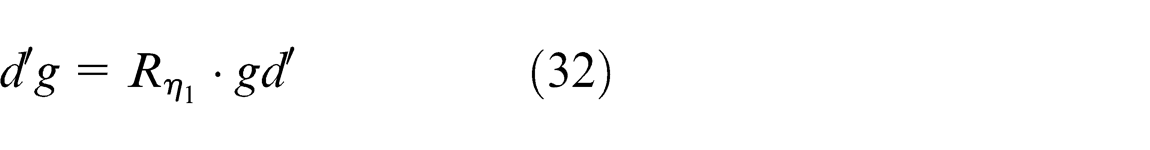
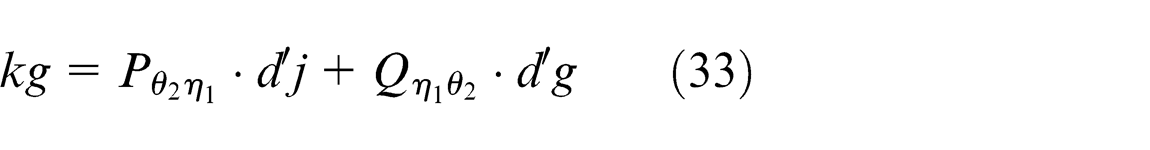
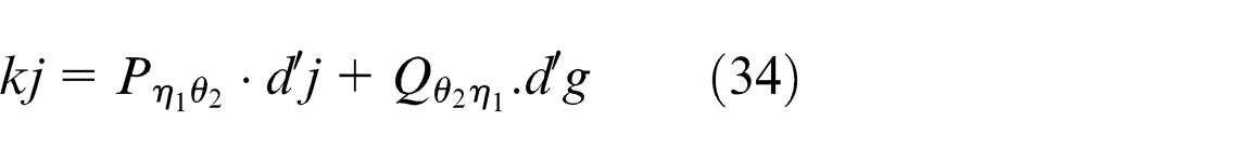
In the gd′jk slip-line, d′j, d′g, kg and kj are given by

d' j = R_{θ_{2}} \cdot jd'

(31)

d' g = R_{η_{1}} \cdot gd'

(32)

kg = P_{θ_{2} η_{1}} \cdot d' j + Q_{η_{1} θ_{2}} \cdot d' g

(33)

kj = P_{η_{1} θ_{2}} \cdot d' j + Q_{θ_{2} η_{1}} . d' g

(34)

In the lg′gk slip-line region, g′l and g′g are expressed as

g' l = P_{θ_{2} δ} \cdot kg + Q_{δ θ_{2}} \cdot kl

(35)

g' g = P_{δ θ_{2}} \cdot kg + Q_{θ_{2} δ} \cdot kl

(36)

In the hg′l slip-line region, hl is determined by

hl = G_{ζ} \cdot g' l

(37)

Equations (2)–(37) have been employed to determine two base slip-lines HL and KJ. After slip-lines HL and KJ are determined, all slip-lines in the secondary shear zone JDSGHLKJ and the transition region ICSDJI and the IA slip-line can be determined by matrix technique.

Determinations of the slip-lines in the primary and tertiary shear zones

The slip-lines in the primary and tertiary shear zones can be determined from relationships between the slip-lines in the new model (Figure 1) and its hodograph (Figure 2), when the slip-lines in the secondary shear zone are determined. The A₃A₂ and B₂N slip-lines are assumed as straight, and the curved slip-lines A ₂ A ₁, I ₁ A ₁, I ₁ C ₁, C ₁ B ₁ and B ₁ B ₂ can be calculated according to equations (38)–(42)

A_{2} A_{1} = Δ S \cdot c

(38)

I_{1} A_{1} = \frac{ρ'}{ρ} \cdot IA

(39)

I_{1} C_{1} = \frac{ρ}{ρ'} \cdot IC

(40)

C_{1} B_{1} = \frac{ρ}{ρ'} \cdot CS

(41)

B_{1} B_{2} = Δ S \cdot c

(42)

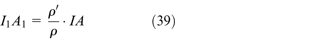
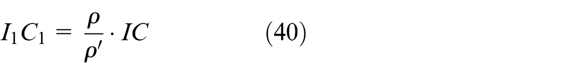
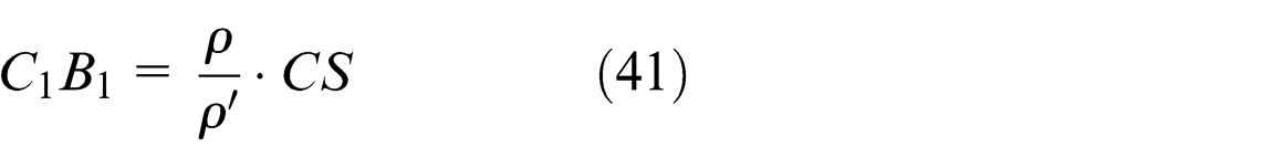
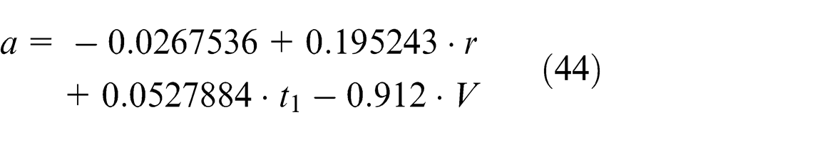
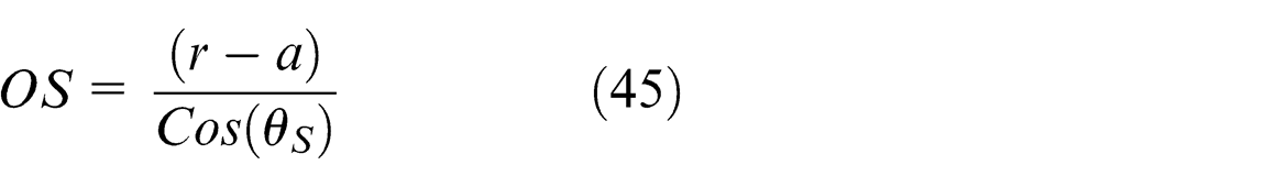
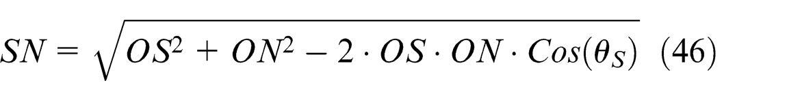
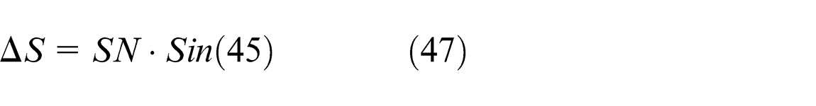
In the above equations, ρ′ is the magnitude of total velocity jump across the slip-lines A ₃ A ₂ A ₁ I ₁ C ₁ B ₁ B ₂ N, ΔS is the thickness of the primary shear zone and the SN slip-line is the length of the bottom side of the dead metal zone and calculated according to equation (47) when it is assumed as straight. Besides, it is assumed that ΔS is equal to SB₂. Equation (44) used to determine the length between the machined surface and the end point of the dead metal zone (separation point S shown in Figure 5) has been taken from Ozturk’s³² work

ON = r

(43)

\begin{matrix} a = - 0.0267536 + 0.195243 \cdot r \\ + 0.0527884 \cdot t_{1} - 0.912 \cdot V \end{matrix}

(44)

OS = \frac{(r - a)}{Cos (θ_{S})}

(45)

SN = \sqrt{{OS}^{2} + {ON}^{2} - 2 \cdot OS \cdot ON \cdot Cos (θ_{S})}

(46)

Δ S = SN \cdot Sin (45)

(47)

Figure 5.

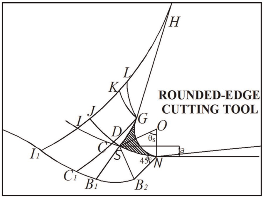
The dead metal zone and the separation angle (θ_S ) in the new slip-line model.

where r is the cutting edge radius, a is the length between the machined surface and the end point of the dead metal zone (separation point S), t ₁ is the uncut chip thickness, V is the cutting speed and θ_S is the separation angle shown in Figure 5.

Determination of the resultant and ploughing forces

The forces and the bending moments are resolved at point I and transmitted through the slip-lines IA, IJ, KJ, KL and HL as shown in Figure 6. Equations (48)–(50) must be satisfied to provide the force and bending moment equilibriums

f_{1} = \sum F_{x} = 0

(48)

f_{2} = \sum F_{y} = 0

(49)

f_{3} = \sum M = 0

(50)

Figure 6.

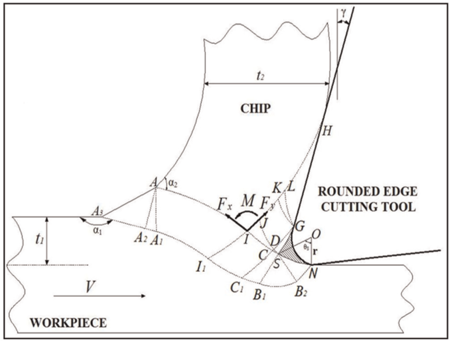
The transmitting of forces and bending moment through slip-lines in the new model.

where the variables f ₁, f ₂ and f ₃ are symbolized three non-linear functions. Powell’s³³ algorithm is performed to solve equations (48)–(50). Equation (51) must be satisfied to provide the force and bending moment equilibriums and to achieve the force-free chip

{(\frac{f_{1}}{{kt}_{1} w})}^{2} + {(\frac{f_{2}}{{kt}_{1} w})}^{2} + {(\frac{f_{3}}{{kt}_{1}^{2} w})}^{2} \leq 10^{- 10}

(51)

where w is the width of cut.

If the forces transmitted through the slip-lines A ₃ A ₂, A ₂ A ₁, I ₁ A ₁, I ₁ C ₁, C ₁ B ₁, B ₁ B ₂ and B ₂ N are denoted by the vectors $F_{A_{3} A_{2}}, F_{A_{2} A_{1}}, F_{I_{1} A_{1}}, F_{I_{1} C_{1}}, F_{C_{1} B_{1}}, F_{B_{1} B_{2}} and F_{B_{2} N}$ , the resultant force (F) can be calculated by adding these seven vectors in equation (52)

\begin{matrix} \frac{F}{{kt}_{1} w} = & \frac{F_{A_{3} A_{2}}}{{kt}_{1} w} + \frac{F_{A_{2} A_{1}}}{{kt}_{1} w} + \frac{F_{I_{1} A_{1}}}{{kt}_{1} w} \\ + \frac{F_{I_{1} C_{1}}}{{kt}_{1} w} + \frac{F_{C_{1} B_{1}}}{{kt}_{1} w} + \frac{F_{B_{1} B_{2}}}{{kt}_{1} w} + \frac{F_{B_{2} N}}{{kt}_{1} w} \end{matrix}

(52)

The cutting force and thrust force can be determined by decomposing the resultant force in the parallel and normal directions to the cutting speed. The ploughing force (P) can be determined according to equation (53)

\frac{P}{{kt}_{1} w} = \frac{F_{B_{1} B_{2}}}{{kt}_{1} w} + \frac{F_{B_{2} N}}{{kt}_{1} w}

(53)

Constraints of stresses and determination of the chip up-curl radius and the chip thickness

According to Hill’s^34,35 overstressing theory, the extension of a stress field into a rigid field is possible for a limited range of solutions of the model for each value of the tool rake angle. For an acceptable solution, the two angles of vertices (α ₁ and α ₂) seen in Figure 1 should not be overstressed, and this condition is mathematically expressed in equations (54) and (55)

\frac{π}{2} - 1 - 2 α_{1} \leq \frac{P_{A}}{k} \leq 2 α_{1} - \frac{3 π}{2} + 1

(54)

2 \cdot Cos (α_{2} - \frac{π}{4}) - 1 \leq \frac{P_{A}}{k} \leq 1 + 2 \cdot (α_{2} - \frac{π}{4})

(55)

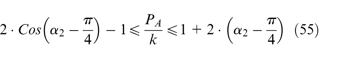
where P_A is the hydrostatic pressure at point A. The two angles of vertices (α ₁ and α ₂) can be determined according to equations (56)–(57)

α_{1} = π - \frac{γ}{2} - \frac{θ_{s}}{2} - δ_{3} - η_{2} - θ_{2} + θ_{1} - δ_{2}

(56)

α_{2} = {Sin}^{- 1} (\frac{V}{ω} \frac{1}{R_{ui}} \sin α_{1})

(57)

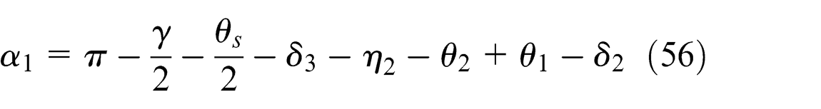
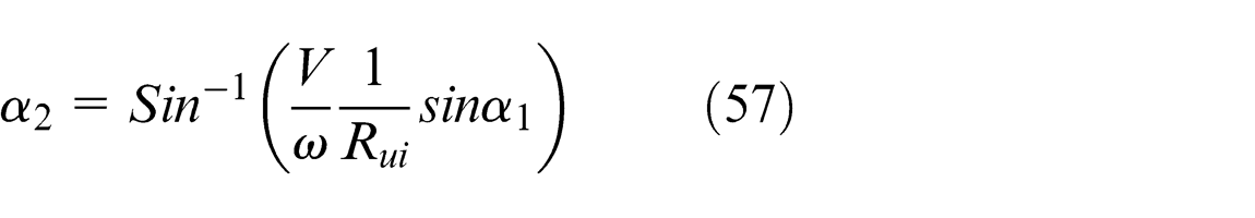
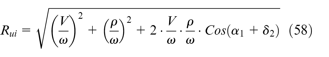
where γ is the tool rake angle and R_ui is the intermediate variable of chip up-curl radius and calculated according to equation (58)

R_{ui} = \sqrt{{(\frac{V}{ω})}^{2} + {(\frac{ρ}{ω})}^{2} + 2 \cdot \frac{V}{ω} \cdot \frac{ρ}{ω} \cdot Cos (α_{1} + δ_{2})}

(58)

Besides, R_u is calculated according to equation (59), and t₂ is the chip thickness and determined according to equation (60)

R_{u} = \frac{R_{ui}}{2} + \frac{V_{h}}{2 ω}

(59)

t_{2} = 2 \cdot (\frac{V_{h}}{ω} - R_{u})

(60)

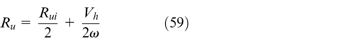
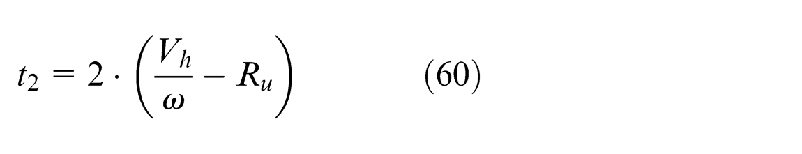
where V_h is the chip speed.

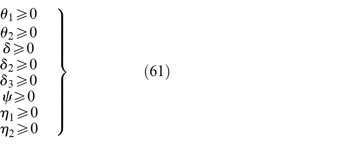
Constraints of slip-line angles

All the eight slip-line angles (θ ₁, θ ₂, δ, δ ₂, δ ₃, ψ, η ₁ and η ₂) must be positive in their numerical value as given in equation (61)

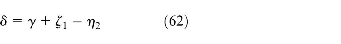
\begin{matrix} \begin{matrix} \begin{matrix} \begin{matrix} \begin{matrix} \begin{matrix} \begin{matrix} θ_{1} \geq 0 \\ θ_{2} \geq 0 \end{matrix} \\ δ \geq 0 \end{matrix} \\ δ_{2} \geq 0 \end{matrix} \\ δ_{3} \geq 0 \end{matrix} \\ ψ \geq 0 \end{matrix} \\ η_{1} \geq 0 \end{matrix} \\ η_{2} \geq 0 \end{matrix}}

(61)

In addition, the slip-line angles have the following relationships

δ = γ + ζ_{1} - η_{2}

(62)

δ_{1} = α_{1} - \frac{3 π}{4}

(63)

δ_{2} = \frac{1}{2} (\frac{P_{A}}{k} - 1)

(64)

δ_{3} = \frac{π}{4} + \frac{γ}{2} - \frac{θ_{s}}{2} + ζ - ψ

(65)

Inputs and outputs of the new slip-line field model

Inputs and outputs of the new slip-line field model are given in Figure 7. The input parameters were used in the equations to determine the slip-lines and to calculate the resultant and ploughing forces. The tool rake angle was used in equations (56), (62) and (65), and the cutting edge radius was used in equations (43)–(45). Machining parameters such as the cutting speed, uncut chip thickness and width of cut were used in equations (44), (52), (53), (57) and (58). Experimental results were performed in equations (44)–(46), (52) and (56), and the stress boundary conditions were used in equations (1), (51)–(55) and (64).

Figure 7.

Inputs and outputs of the new slip-line field model.

Experimental study

In this study, a shaping-based quick stop device (QSD) was used in experiments (Figure 8). The QSD was developed to collect the chip-root samples. It is necessary to effectively freeze the cutting action without substantially disturbing the state of the chip. There are two basic motions in this QSD. One of them is cutting and the other is sensitive depth-of-cut motions. Brass (CuZn30) was chosen as workpiece material. Chemical composition of the samples was Cu% = 69.73, Zn% = 30.216, Pb% = 0.006, Fe% = 0.008 and Ni% = 0.04, and the yield strength, the tensile strength, the elongation and the elastic modulus were 320 MPa, 440 MPa, 11% and 114 GPa, respectively. The dimensions of the workpieces were set as 32 × 30 × 1.5 mm³ by laser cutting and the depth of heat-affected zone was measured as 60 μm by Bulut Machine HVS-1000 micro-hardness device. Therefore, the uncut chip thicknesses were chosen more than 60 μm. Uncoated tungsten carbide (WC) cutting tool inserts were chosen as TPGN160308.

Figure 8.

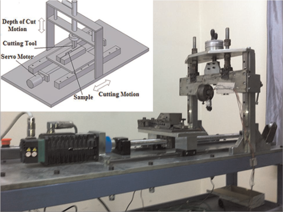
Shaping-based quick stop device.

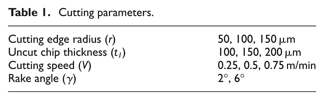
All 54 experiments were performed with various cutting edge radii, uncut chip thicknesses, cutting speeds and rake angles. Cutting parameters are given in Table 1. Cutting edge radii were measured by the optical measuring system.

Table 1.

Cutting parameters.

Cutting edge radius (r)	50, 100, 150 µm
Uncut chip thickness (t₁ )	100, 150, 200 µm
Cutting speed (V)	0.25, 0.5, 0.75 m/min
Rake angle (γ)	2°, 6°

Brass samples were machined by the shaping-based QSD. The workpiece was not cut along the length and the chip was not broken to investigate the dead metal zone. The sanding and polishing operations of the samples were performed using MetaServ 2000 Sander/Polisher device. Then, the samples were etched by etchant including 100 mL H₂O, 96 mL ethanol and 59 g FeCl₃, as given in Voort’s³⁶ study. Investigation of these etched brass samples was carried out by SOIF XJP-2 optical microscope. Dead metal zone microphotographs were observed for the rounded-edge cutting tools (Figure 9).

Figure 9.

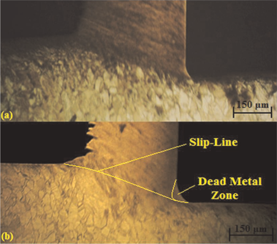
Microphotographs of the dead metal zone for rounded-edge cutting tools of V = 0.5 m/min, t ₁ = 150 μm and γ = 2°: (a) r = 50 μm and (b) r = 100 μm.

Results and discussions

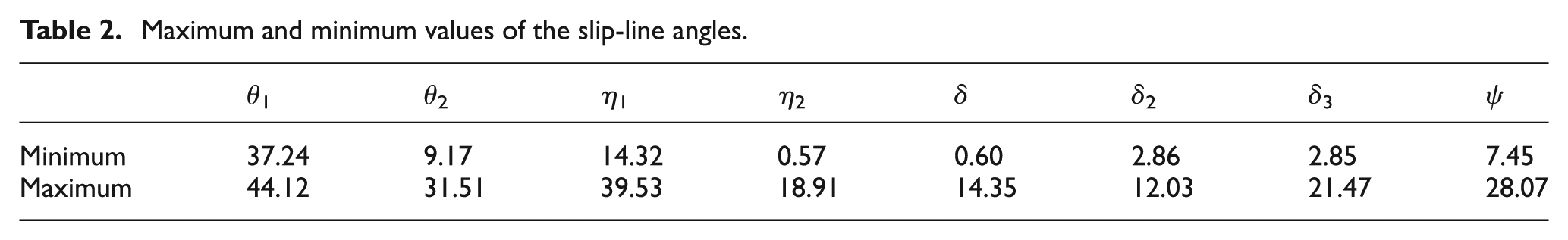
Mathematical formulations of the new slip-line field model were solved by MATLAB^® software. The values of P_A /k and τ/k were assumed to be 1.1 and 0.9, respectively, from Fang’s²¹ and Fang and Jawahir’s³⁷ studies. The separation angle (θ_S ) was chosen as 60° from Fang’s²¹ work and Ozturk’s³² experimental study. Besides, the length between the machined surface and the end point of the dead metal zone (a) was calculated using equation (44) based on Ozturk’s³² work. The approach to solve the new slip-line field model was taken to be 1%. All variables were solved by equalizing the resultant force obtained from the computer-controlled QSD to the resultant force obtained from the new model. The slip-line angles were obtained by solving the model and the maximum and minimum values are given in Table 2.

Table 2.

Maximum and minimum values of the slip-line angles.

	θ ₁	θ ₂	η ₁	η ₂	δ	δ ₂	δ ₃	ψ
Minimum	37.24	9.17	14.32	0.57	0.60	2.86	2.85	7.45
Maximum	44.12	31.51	39.53	18.91	14.35	12.03	21.47	28.07

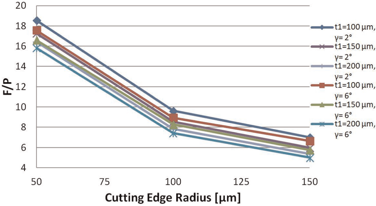
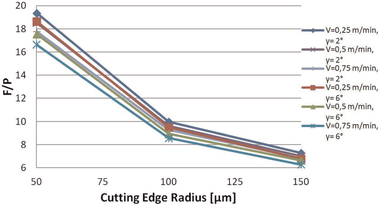
The effects of cutting edge radius and uncut chip thickness on the ploughing force are given in Figures 10 and 11, respectively. Besides, the change in the ratio of the resultant force to the ploughing force according to the cutting edge radius and uncut chip thickness can be seen in Figures 12 –15.

Figure 10.

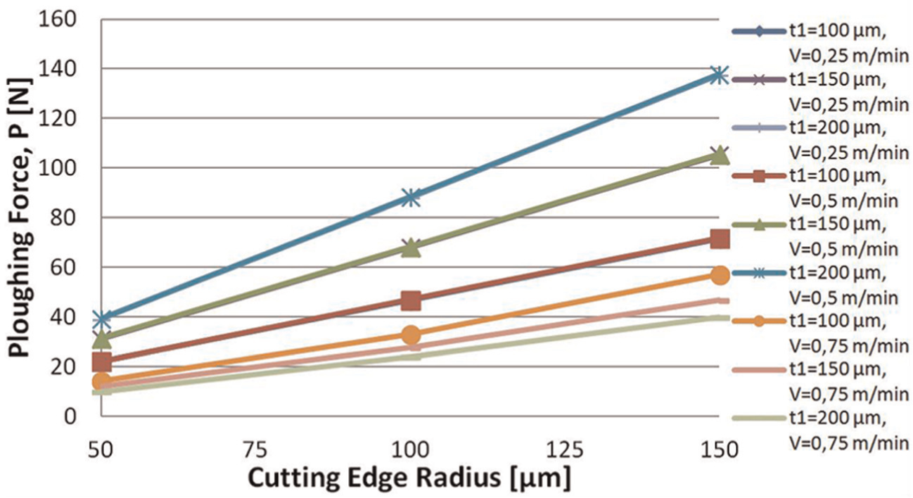
Effect of cutting edge radius on ploughing force, γ = 2°.

Figure 11.

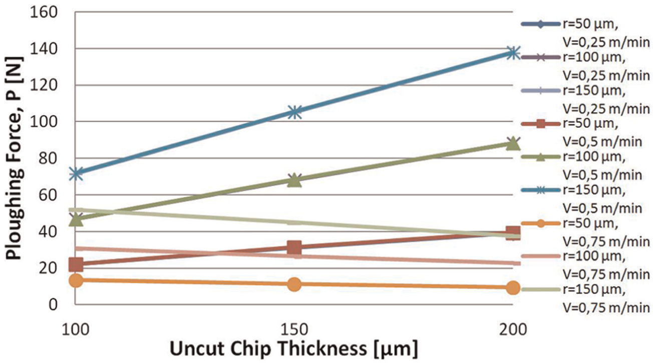
Effect of uncut chip thickness on ploughing force, γ = 6°.

Figure 12.

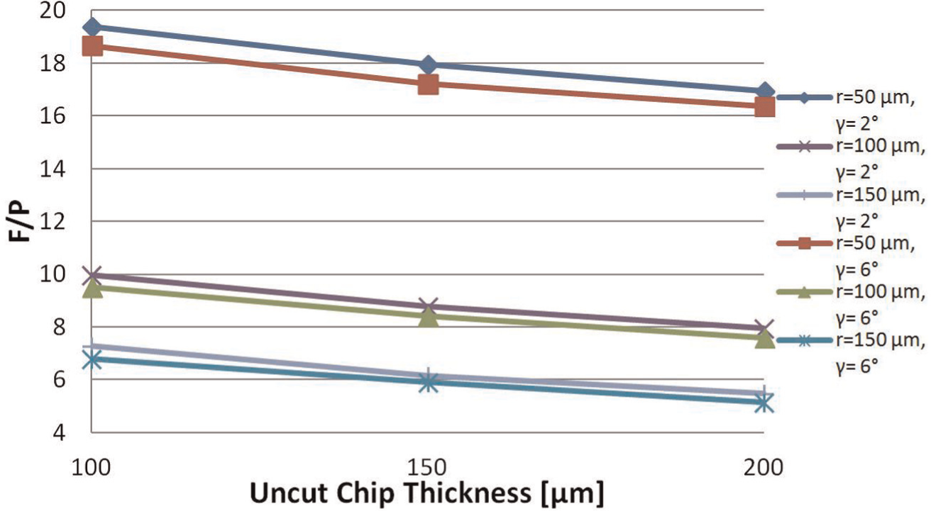
Effect of cutting edge radius on the ratio of resultant force to ploughing force, V = 0.5 m/min.

Figure 13.

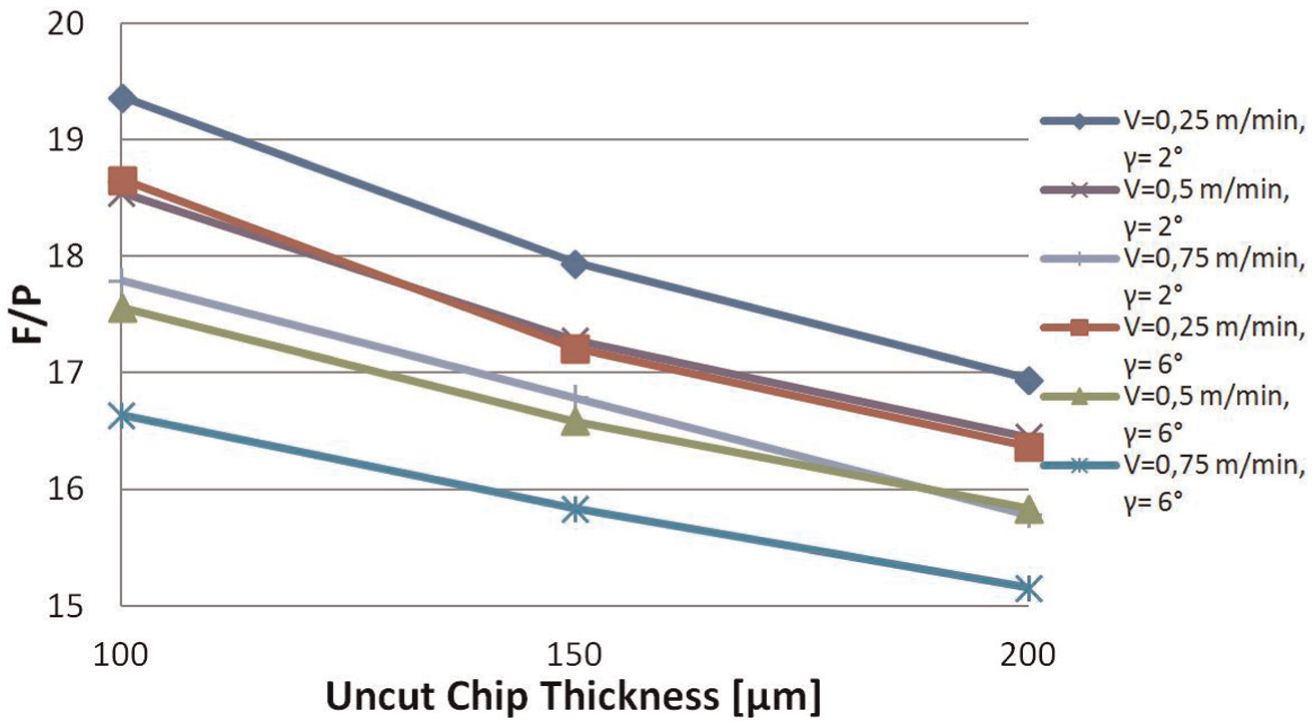
Effect of cutting edge radius on the ratio of resultant force to ploughing force, t₁ = 100 μm.

Figure 14.

Effect of uncut chip thickness on the ratio of resultant force to ploughing force, V = 0.25 m/min.

Figure 15.

Effect of uncut chip thickness on the ratio of resultant force to ploughing force, r = 50 μm.

The ploughing force increased when the cutting edge radius increased as shown in Figure 10. It was specified that the effect of ploughing force on the resultant force increased as the cutting edge radius increased (Figures 12 and 13) because higher cutting edge radius made the ploughing process of the cutting tool difficult. The change in the ratio of the resultant force to the ploughing force was affected by the cutting speed very much as the cutting edge radius decreased. It was seen that the effect of the ploughing force on the resultant force decreased slightly with an increase in the cutting speed (seen in Figure 15) and the rake angle (seen in Figures 12 –15). For given cutting conditions, the ratio of resultant force to ploughing force decreased when the cutting speed increased due to the fact that the increase in the cutting speed reduced the dead metal zone formation and this caused the decrease in the ploughing force.

The ploughing force increased with a cutting speed of 0.25 and 0.5 m/min as given in Figure 11. It decreased with a cutting speed of 0.75 m/min when the uncut chip thickness increased. In addition, it was specified that the effect of ploughing force on the resultant force increased with an increase in uncut chip thickness (Figures 14 and 15).

Effects of the cutting edge radius and the uncut chip thickness on the primary shear zone (ΔS) and the length of the bottom side of the dead metal (SN) are given in Figures 16 –19.

Figure 16.

Effect of cutting edge radius on the primary shear zone thickness, V = 0.5 m/min.

Figure 17.

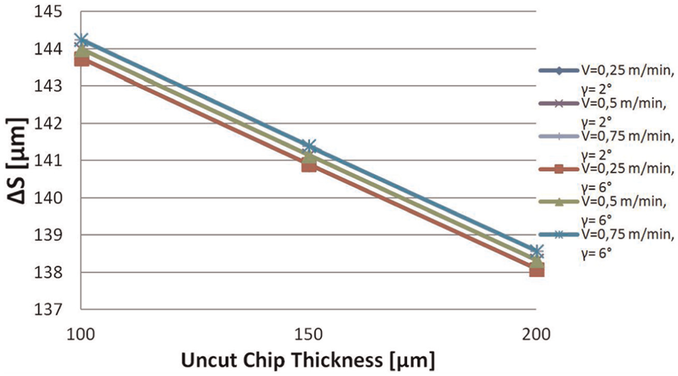
Effect of uncut chip thickness on the primary shear zone thickness, r = 150 μm.

Figure 18.

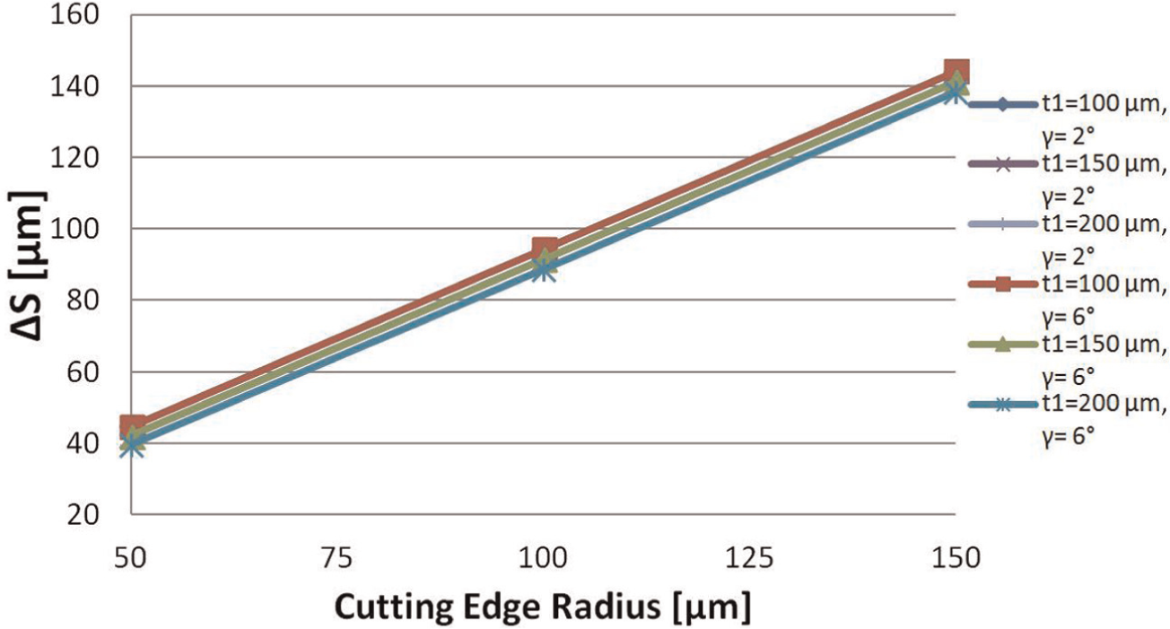
Effect of cutting edge radius on the length of the bottom side of the dead metal, V = 0.75 m/min.

Figure 19.

Effect of uncut chip thickness on the length of the bottom side of the dead metal, r = 50 μm.

The primary shear zone thickness (ΔS) increased with the increase in the cutting edge radius, decreased slightly with the increase in the uncut chip thickness, and it did not change with the cutting speed and rake angle very much as shown in Figures 16 and 17.

The length of the bottom side of the dead metal zone (SN) increased as the cutting edge radius increased and decreased a little when the uncut chip thickness increased (Figures 18 and 19). Besides, it did not change with cutting speed very much. The size of the dead metal zone grew as the length of the bottom side of the dead metal zone increased. Therefore, it can be pointed that the reason of increasing the ploughing force with the increase in the cutting edge radius was the growing of dead metal zone size.

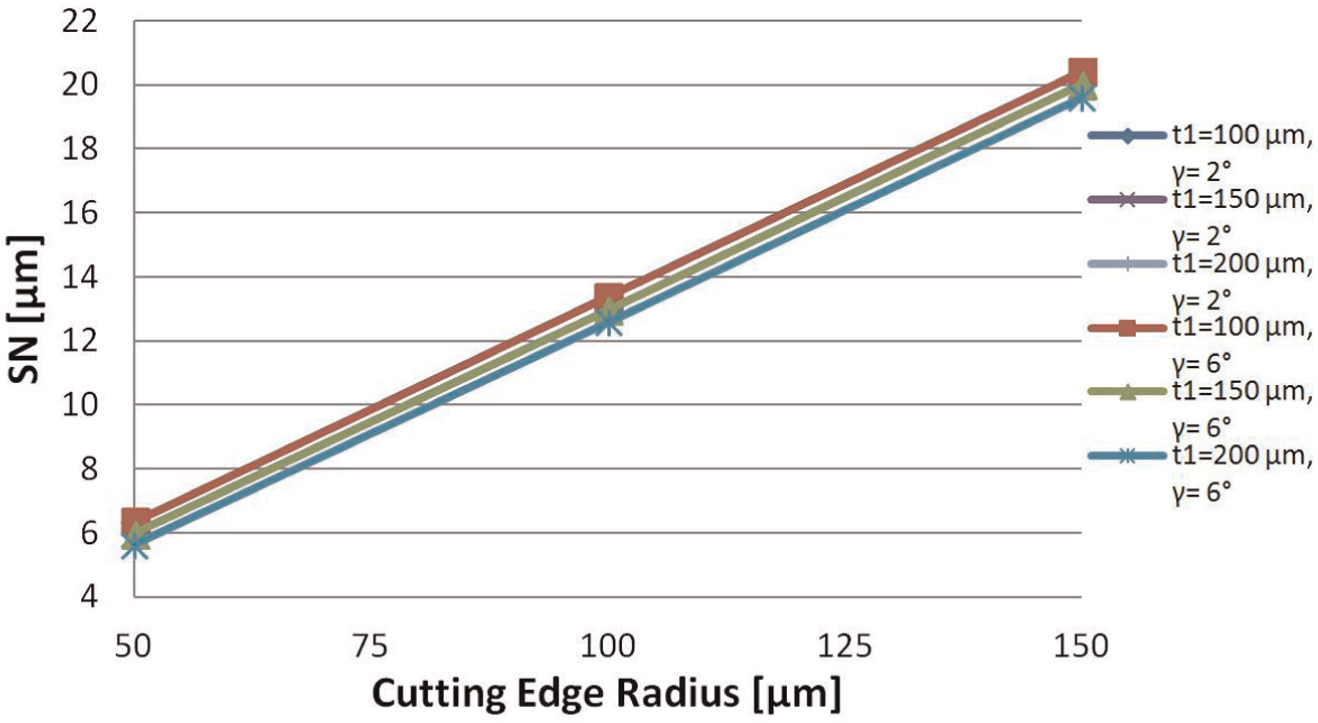
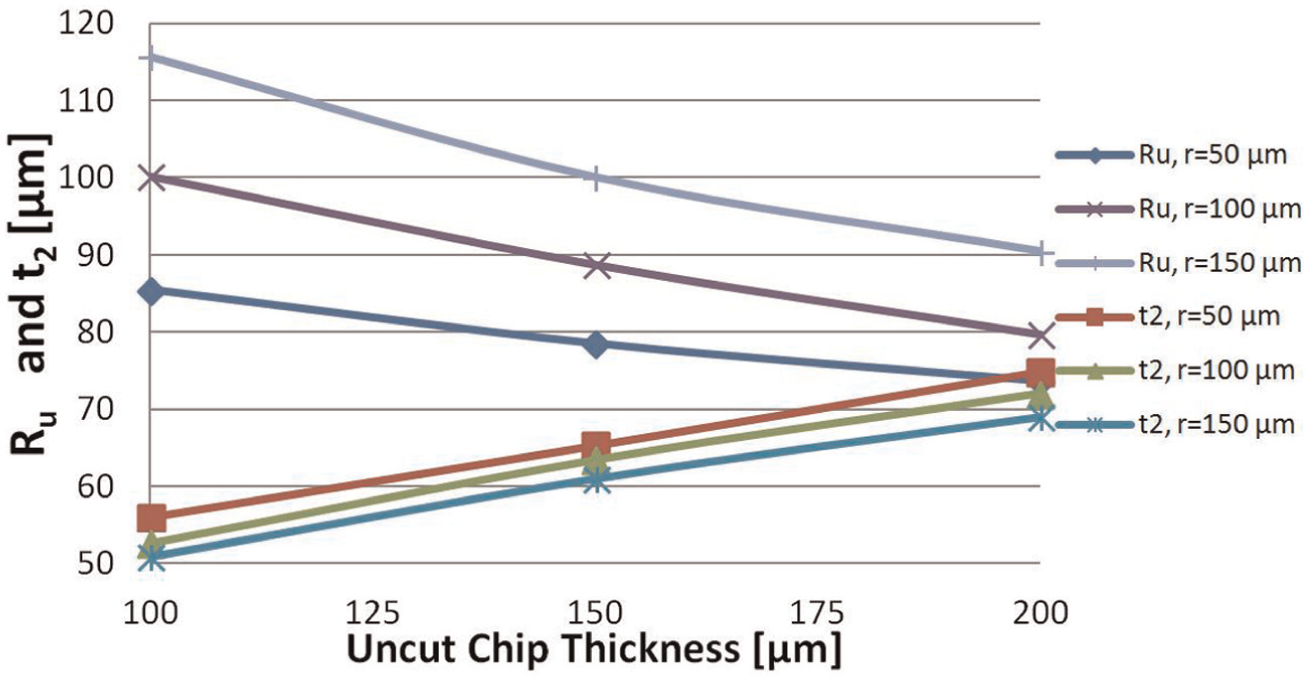
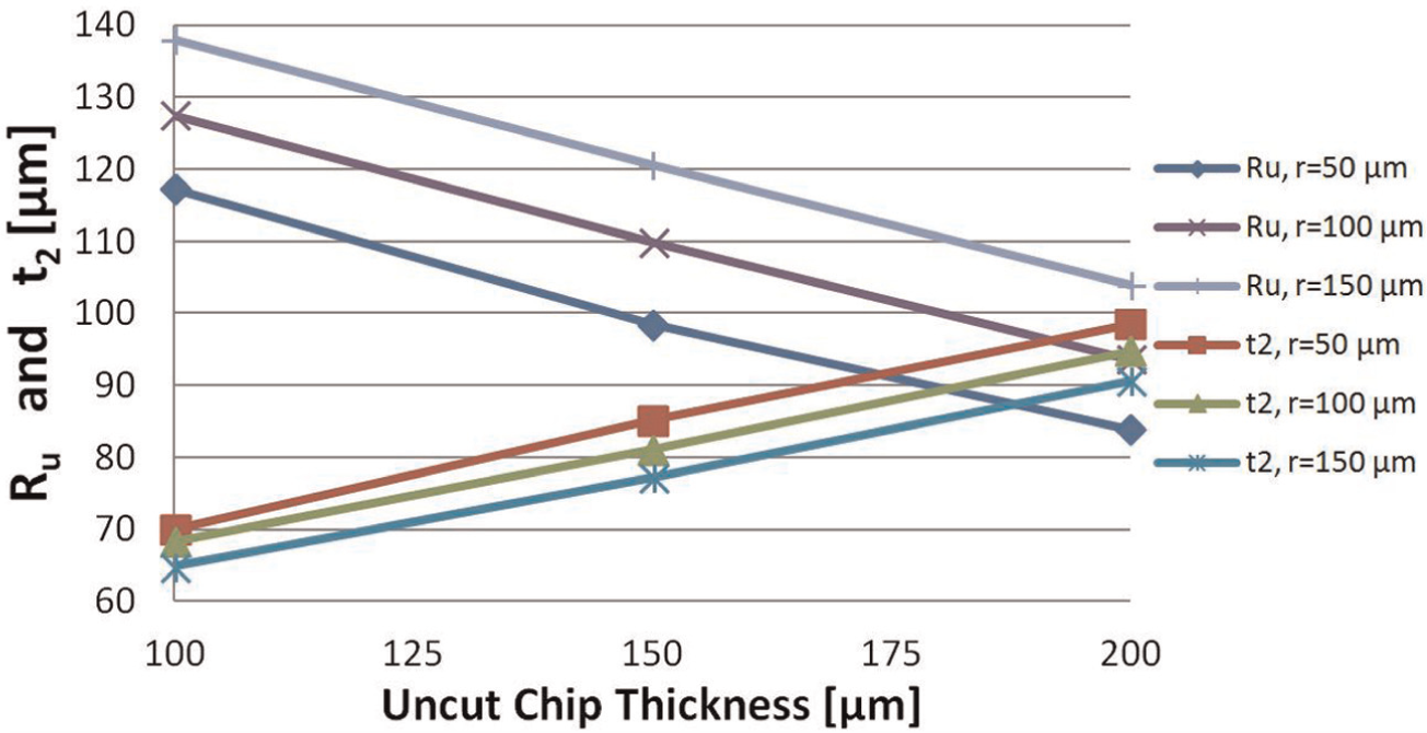
The effects of the cutting edge radius and the uncut chip thickness on the chip up-curl radius (R_u ) and the chip thickness (t₂ ) are given in Figures 20 –23.

Figure 20.

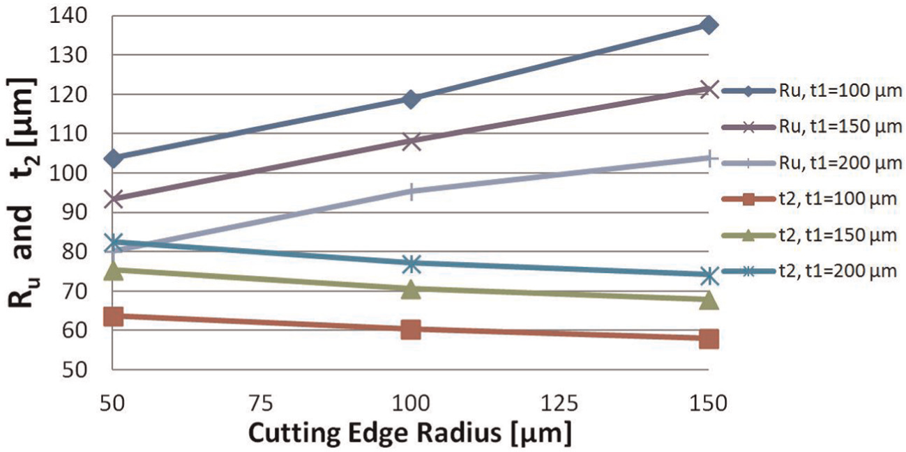
Effect of the cutting edge radius on the chip up-curl radius and chip thickness, V = 0.5 m/min, γ = 2°.

Figure 21.

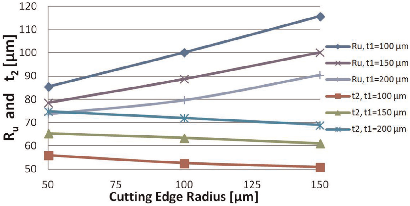
Effect of the cutting edge radius on the chip up-curl radius and chip thickness, V = 0.75 m/min, γ = 2°.

Figure 22.

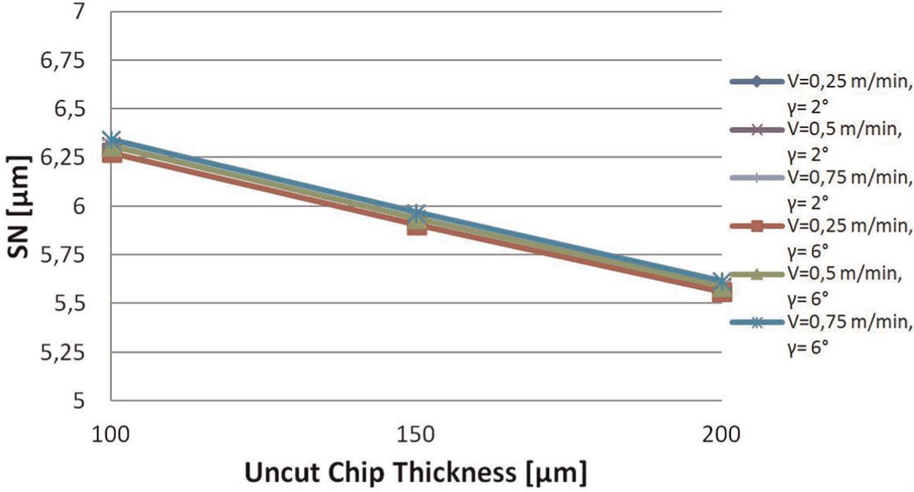
Effect of uncut chip thickness on the chip up-curl radius and chip thickness, V = 0.75 m/min, γ = 2°.

Figure 23.

Effect of uncut chip thickness on the chip up-curl radius and chip thickness, V = 0.75 m/min, γ = 6°.

The chip-breaking process and the chip formation were affected by the chip up-curl radius (R_u ). It was observed that the chip up-curl radius increased when the cutting edge radius increased. Thus, longer chips were obtained with an increase in the chip up-curl radius (Figures 20 and 21). Additionally, it was seen that the chip up-curl radius decreased with an increase in the uncut chip thickness, and the increase in uncut chip thickness made the chip curling difficult (Figures 22 and 23). Besides, the chip up-curl radius increased as the rake angle increased and decreased as the cutting speed increased. It was specified that the chip thickness (t₂ ) decreased slightly when the cutting edge radius rose and increased when the uncut chip thickness increased. In addition, the chip thickness increased with the increase in the rake angle and decreased with the increase in the cutting speed (Figures 20 –23).

Conclusion

In this study, a new slip-line field model for orthogonal machining with a rounded-edge cutting tool was developed. The proposed slip-line model simultaneously predicted the resultant force, ploughing force, primary shear zone, length of the bottom side of the dead metal zone, chip up-curl radius and chip thickness. The mathematical formulations of the new model and hodograph were developed based on the basic matrix algorithm of Dewhurst and Collins.³⁰ The results obtained from solving the new slip-line model and hodograph are as follows:

The mathematical formulation of the new model was calculated by equalizing the resultant force obtained from the slip-line field model to the experimental resultant force. The approach to solve the new slip-line field model was taken to be1%. Therefore, the new model results were consistent with the experimental results.

It was specified that the ploughing force efficiency on the resultant force increased with the increase in the cutting edge radius.

The ratio of the resultant force to the ploughing force was much more affected by the cutting speed with the reduction in the cutting edge radius.

It was seen that the ploughing force efficiency decreased as the rake angle and the cutting speed increased. Besides, it was specified that the ploughing force was most affected by the cutting edge radius in machining with a rounded-edge cutting tool.

The ploughing force usually increased with the increase in the uncut chip thickness. In addition, it was seen that the effect of ploughing force on the resultant force increased as the uncut chip thickness increased.

It was specified that the primary shear zone thickness (ΔS) increased with the increase in the cutting edge radius, decreased a little with the increase in the uncut chip thickness, and it did not change with the cutting speed and rake angle very much.

It was defined that the length of the bottom side of the dead metal zone (SN) increased as the cutting edge radius increased and decreased slightly when the uncut chip thickness increased. It was specified that it did not change with the cutting speed very much.

It was seen that the chip up-curl radius (R_u ) increased with an increase in the cutting edge radius and decreased with an increase in the uncut chip thickness. Furthermore, the chip up-curl radius increased as the rake angle increased and decreased as the cutting speed increased.

It was specified that the chip thickness (t₂ ) decreased a little when the cutting edge radius increased and increased when the uncut chip thickness increased. In addition, the chip thickness increased with the increase in the rake angle and decreased with the increase in the cutting speed.

Footnotes

Appendix 1

Appendix 2

The computational flow chart of the new slip-line model is given in Figure 24.

Appendix 3

In this study, P, P*, Q, Q*, R and G are the basic matrix operators defined by Dewhurst and Collins³⁰ which were used to solve the developed slip-line model. According to the researchers’ study, a slip-line is to be thought of as being represented by the column vector of coefficients in the series expansion of its radius of curvature. Thus, the curves and flow directions forming the slip-lines can be defined by mathematical expressions.

The column vector coefficients of the curves are expressed as equation (66)

(66)

\begin{matrix} σ_{1} = [\begin{matrix} \begin{matrix} a_{0} \\ a_{1} \end{matrix} \\ a_{2} \\ ⋮ \end{matrix}] & σ_{2} = [\begin{matrix} \begin{matrix} b_{0} \\ b_{1} \end{matrix} \\ b_{2} \\ ⋮ \end{matrix}] \\ σ_{3} = [\begin{matrix} \begin{matrix} r_{0} \\ r_{1} \end{matrix} \\ r_{2} \\ ⋮ \end{matrix}] & σ_{4} = [\begin{matrix} \begin{matrix} s_{0} \\ s_{1} \end{matrix} \\ s_{2} \\ ⋮ \end{matrix}] \end{matrix}}

These latter components are related to those of σ ₁ and σ ₂ and can be written in matrix form as equation (67)

(67)

\begin{matrix} σ_{3} = P_{ψ}^{*} σ_{1} + Q_{ψ}^{*} σ_{2} \\ σ_{4} = P_{θ}^{*} σ_{2} + Q_{θ}^{*} σ_{1} \end{matrix}}

where

(68)

P_{θ}^{*} = [\begin{matrix} θ_{0} & 0 & 0 & \dots \\ θ_{1} & θ_{0} & 0 & \dots \\ θ_{2} & θ_{1} & θ_{0} & \dots \\ ⋮ & ⋮ & ⋮ & ⋮ \end{matrix}]

and

(69)

Q_{θ}^{*} = - [\begin{matrix} θ_{1} & θ_{2} & θ_{3} & \dots \\ θ_{2} & θ_{3} & θ_{4} & \dots \\ θ_{3} & θ_{4} & θ_{5} & \dots \\ ⋮ & ⋮ & ⋮ & ⋮ \end{matrix}]

where

(70)

θ_{m} = \frac{θ^{m}}{m!}

The significance of the P* and Q* matrix operators can be seen by considering the special case in which one of the base slip-lines (σ ₂) degenerates into a point (σ ₂ = 0 in equation (67)). P* and Q* are hence the matrix operators which generate the singular field on the convex side of a given slip-line. From equation (67), therefore, it is evident that the curves σ ₃ and σ ₄ can be regarded as the sum of certain curves in the singular fields constructed on the two base curves σ ₁ and σ ₂.

We now define the unstarred P and Q matrices by equation (71)

(71)

P_{θ ψ} = R_{θ} P_{ψ}^{*} and Q_{θ ψ} = R_{ψ} Q_{θ}^{*}

where R_θ and R_ψ are reversion matrix operators. For example, R_ψ reverses the intrinsic direction of a given slip-line with angular span ψ

(72)

R_{ψ} = - [\begin{matrix} ψ_{0} & ψ_{1} & ψ_{2} & \dots \\ 0 & - ψ_{0} & - ψ_{1} & \dots \\ 0 & 0 & ψ_{0} & \dots \\ ⋮ & ⋮ & ⋮ & ⋮ \end{matrix}]

When the intrinsic directions of σ ₃ and σ ₄ are opposite to those in equation (67), the mathematical expressions are represented as equation (73)

(73)

\begin{matrix} σ_{3} = P_{θ ψ} σ_{1} + Q_{ψ θ} σ_{2} \\ σ_{4} = P_{ψ θ} σ_{1} + Q_{θ ψ} σ_{2} \end{matrix}}

When a slip-line makes an angle λ with a rough straight boundary, the G matrix operator (equation (74)) is used

(74)

G_{λ} = Q_{θ θ} + P_{θ θ} {(Icos λ - Jsin λ)}^{- 1} (Jcos λ - Isin λ)

where I is the unit matrix, and J is expressed as equation (75)

(75)

J = [\begin{matrix} 0 & 0 & 0 & \dots \\ 1 & 0 & 0 & \dots \\ 0 & 1 & 0 & \dots \\ ⋮ & ⋮ & ⋮ & ⋮ \end{matrix}]

Declaration of conflicting interests

The authors declare that there is no conflict of interest.

Funding

This research has been supported by Yildiz Technical University Scientific Research Projects Coordination Department. Project Number: 29-06-01-DOP01.

References

Merchant

. Basic mechanics of the metal cutting process. J Appl Mech: T ASME 1941; 66: A168–A175.

Lee

Shaffer

. The theory of plasticity applied to a problem of machining. J Appl Mech: T ASME 1951; 73: 405–413.

Oxley

PLB

. The mechanics of machining: an analytical approach to assessing machinability. Chichester: Ellis Horwood Limited, 1989.

Maity

Das

. A slip-line solution to metal machining using a cutting tool with a step-type chip-breaker. J Mater Process Tech 1998; 79: 217–223.

Maity

Das

. A class of slip-line field solutions for metal machining with elastic contact. J Mater Process Tech 1999; 96: 9–18.

Maity

Das

. A class of slip-line field solutions for metal machining with Coulomb friction at the chip–tool interface. J Mater Process Tech 2001; 116: 278–288.

Maity

Das

. A class of slipline field solutions for metal machining with slipping and sticking contact at the chip-tool interface. Int J Mech Sci 2001; 43: 2435–2452.

Fang

Jawahir

Oxley

PLB

. A universal slip-line model with non-unique solutions for machining with curled chip formation and a restricted contact tool. Int J Mech Sci 2001; 43: 557–580.

Fang

. Machining with tool–chip contact on the tool secondary rake face – part I: a new slip-line model. Int J Mech Sci 2002; 44: 2337–2354.

10.

Fang

. Machining with tool–chip contact on the tool secondary rake face – part II: analysis and discussion. Int J Mech Sci 2002; 44: 2355–2368.

11.

Das

Chawla

Biswas

. An analysis of strain in chip breaking using slip-line field theory with adhesion friction at chip/tool interface. J Mater Process Tech 2005; 170: 509–515.

12.

Kudo

. Some new slip-line solutions for two dimensional steady state machining. Int J Mech Sci 1965; 7: 43–55.

13.

Fang

Dewhurst

. Slip-line modeling of built-up edge formation in machining. Int J Mech Sci 2005; 47: 1079–1098.

14.

Das

Dundur

. A slipline field analysis of free-chip orthogonal machining with adhesion friction at rake face. Mach Sci Technol 2006; 10: 371–387.

15.

Xue

Tong

. Slip-line field modeling of orthogonal machining pressure sensitive materials. Int J Adv Manuf Tech 2012; 58: 907–914.

16.

Albrecht

. New developments in the theory of the metal cutting process: the ploughing process in metal cutting. J Eng Ind 1960; 81: 348–358.

17.

Abdelmoneim

MES

Scrutton

. Tool edge roundness and stable build-up formation in finish machining. J Eng Ind 1974; 96: 1258–1267.

18.

Abdelmoneim

MES

. Tool edge roundness in finish machining at high cutting speeds. Wear 1980; 58: 173–192.

19.

Waldorf

DeVor

Kapoor

. A slip-line field for ploughing during orthogonal cutting. J Manuf Sci E: T ASME 1998; 120: 693–699.

20.

Fang

. Slip-line modeling of machining with a rounded-edge tool – part I: new model and theory. J Mech Phys Solids 2003; 51: 715–742.

21.

Fang

. Slip-line modeling of machining with a rounded-edge tool – part II: analysis of the size effect and the shear strain-rate. J Mech Phys Solids 2003; 51: 743–762.

22.

Fang

. Theoretical and experimental investigations of finish machining with a rounded edge tool. J Mater Process Tech 2007; 191: 331–334.

23.

Wang

Jawahir

. Recent advances in plasticity applications in metal machining: slip-line models for machining with rounded cutting edge restricted contact grooved tools. Int J Mach Mach Mater 2007; 2: 347–360.

24.

Karpat

Ozel

. Mechanics of high speed cutting with curvilinear edge tools. Int J Mach Tool Manu 2008; 48: 195–208.

25.

Jin

Altintas

. Slip-line field model of micro-cutting process with round tool edge effect. J Mater Process Tech 2011; 211: 339–355.

26.

Uysal

Ozturk

Altan

. A slip-line approach to the micro-cutting process with a rounded-edge tool. Adv Mat Res 2012; 445: 56–61.

27.

Ozturk

Altan

. A slip-line approach to the machining with rounded-edge tool. Int J Adv Manuf Tech 2012; 63: 513–522.

28.

Ozturk

Uysal

Altan

. Metallographic analysis of the dead metal zone in metal cutting with a rounded-edge tool. Prakt Metallogr: Pr M 2013; 50: 318–330.

29.

Ozturk

Altan

. Position of the separation point in machining with a rounded-edge tool. Proc IMechE, Part B: J Engineering Manufacture 2013; 227: 965–971.

30.

Dewhurst

Collins

. A matrix technique constructing slip-line field solutions to a class of plane strain plasticity problems. Int J Numer Meth Eng 1973; 7: 357–378.

31.

Green

. On the use of hodographs in problems of plane plastic strain. J Mech Phys Solids 1954; 2: 73–80.

32.

Ozturk

. Investigation and modeling of cutting forces by using material flow on orthogonal cutting with a rounded-edge cutting tool. PhD Thesis, Yildiz Technical University, Istanbul, Turkey, 2009 (in Turkish).

33.

Powell

MJD

. A fortran subroutine for solving systems of non-linear algebraic equations. London: Gordon and Breach, 1970.

34.

Hill

. The mechanics of machining: a new approach. J Mech Phys Solids 1954; 3: 47–53.

35.

Hill

. On the limits set by plastic yielding to the intensity of singularities of stress. J Mech Phys Solids 1954; 2: 278–285.

36.

Voort

GFV

. ASM handbook: volume 9: metallography and microstructures. Materials Park, OH: ASM International, 2004.

37.

Fang

Jawahir

. Analytical predictions and experimental validation of cutting force ratio, chip thickness and chip back-flow angle in restricted contact machining using the universal slip-line model. Int J Mach Tool Manu 2002; 42: 681–694.

Slip-line field modelling of rounded-edge cutting tool for orthogonal machining

Abstract

Keywords

Introduction

The new slip-line field model

Mathematical formulation of the new slip-line field model

Determination of the tool–chip friction

Determination of the slip-lines in the secondary shear zone

Relationships among the slip-lines in the proposed new slip-line model

Relationships among the slip-lines in the hodograph of the proposed new slip-line model

Determinations of the slip-lines in the primary and tertiary shear zones

Determination of the resultant and ploughing forces

Constraints of stresses and determination of the chip up-curl radius and the chip thickness

Constraints of slip-line angles

Inputs and outputs of the new slip-line field model

Experimental study

Results and discussions

Conclusion

Footnotes

Appendix 1

Appendix 2

Appendix 3

Declaration of conflicting interests

Funding

References