Multipart setup planning through integration of process planning and scheduling

Abstract

The importance of integration of process planning and scheduling is evident in today’s competitive manufacturing system. Meanwhile, the setup planning plays an important role for integration, because setup planning is done after process planning, just before scheduling. In this article, a new approach for setup planning for multiparts is introduced to realize integration of process planning and scheduling with more details of manufacturing constraints for setup planning. For this purpose, the necessary and unnecessary (preferred) constraints are defined for setup formation and a new matrix is presented to distinguish these and to specify the precedence of operations. The simulated annealing is used in setup planning for N parts simultaneously based on multi-technical and scheduling objectives. The proposed system is based on the machining operation instead of features, to select machine tools more accurately. Another factor for the selection of machine tools is tolerances that are considered in this article and greatly affected the machining cost. An illustrative example is presented to show the effectiveness of the operation-based system and the second example is presented to demonstrate the influence of multipart setup planning versus single-part setup planning. The results show that considering multiparts improves the scheduling objectives such as makespan.

Introduction

In the competitive market of today, companies can be growing which are able to adopt themselves to the rapid change in the market demand. In this way, the integration of process planning and scheduling (IPPS) plays an important role in the manufacturing system. In the past, process planning and scheduling have been treated as separate systems with different objectives. Process planning systems focus on systematic determination of methods by which design requirements have been complied with little attention to the shop floor status.

On the other hand, the industrial development has led to more complex scheduling problem. The modern machines, generally, require a shorter processing time for performing the same operations as the older machines. It is well known that a combinatorial problem such as job shop scheduling problem (JSSP) presents a nonlinear multi-peak objective function in the multidimensional searching space. Thus, undirected searching techniques or branch and bound methods, in the worst case, take an unacceptable computational time to produce a solution close to the optimum; therefore, presentation of the most efficient heuristic algorithm has been the main concern of the scheduling research area. ¹

Today’s manufacturing environment is quite different from the traditional one. It is characterized by decreasing lead time, exacting standards of quality, larger part variety and competitive costs. In such manufacturing environment, it is difficult to get a satisfactory result using traditional approach. ² If a process plan is determined without considering the availability of shop resources, it may become unfeasible owing to probable constraints and changes in the manufacturing workshop. ³

Over the last decades, several methods and algorithms have been reported in the literatures for IPPS. The biggest problem is thus the complexity of the problems which limit the achievements of the integration.

Setup planning is identifying the proper setups to be used when machining a part, the number of setups and the sequence of setups and sequencing of operations in each setup. Therefore, setup planning must consider constraints of design specification and manufacturing resources including availability of machine tools and their capabilities, simultaneously. As a result, setup planning is done after process planning, just before scheduling. Thus, it is obvious that setup planning plays an important role in the IPPS.

The literature reviews reveal that the flexibility of setup planning has not been fully addressed, especially from a process planning and scheduling integration point of view. ⁴ A few researches that focused on this point such as Wang et al. ⁴ and Mohapatra et al. ⁵ suffer from two big problems:

1. They proposed an approach that is proper for one part, while the IPPS has N parts.

2. Manufacturing constraints that affect the setup planning are partially considered as their availability and other constraints especially machine tool capabilities (such as accuracy) have been ignored.

This article presents an approach to integrate process planning and scheduling for multiparts with more details on setup planning which considers the manufacturing constraints. The remaining part of the article is organized as follows: section “Literature review” reviews literatures. Section “Representation of the setup planning system” represents the setup planning system; the proposed optimization algorithm is defined in section “Proposed algorithm.” An example is illustrated in section “Illustrative example” and finally, the conclusion is presented in section “Conclusion.”

Literature review

The IPPS is defined as follows. ⁶ Given a set of N parts that are to be processed on m machines with operations including alternative manufacturing resources (machines, tools and tool approach directions (TADs)), select suitable manufacturing resources and sequence the operations so as to determine a schedule in which the precedence constraints among operations can be satisfied and the corresponding objectives can be achieved.

There are two general approaches for IPPS: progressive (distributed) approach and centralized (simultaneous) approach. In the progressive e approach, the process planning system generates a reasonable alternative process plan for each part before it enters into the shop floor and then in production time, a schedule can be determined by iteratively selecting a suitable process plan from alternative plans of each part until a satisfactory performance is achieved. ⁶ Jain et al. ⁷ proposed a method to take advantage of this approach, while following a real-time strategy for scheduling. Haddadzade et al. ⁸ proposed a progressive approach to avoid dismantling existing departments in a company.

In a simultaneous approach, the process planning and scheduling are both in dynamic adjustments until specific performance criteria are satisfied. ⁹ In this approach, a closer IPPS is achieved by dynamic interactions and information sharing between these two functions. ¹⁰ Leung et al. ¹¹ used this approach for an agent-based job shop environment. Li and McMahon ¹⁰ represented a unified model to integrate process planning and scheduling more tightly to achieve the global optimization. Bensmaine et al. ¹² proposed a heuristic algorithm to IPPS problem for reconfigurable manufacturing systems and the results were compared with the sequential process planning and scheduling in which the results showed that the makespan is reduced with their algorithm. Lv and Qiao ¹³ proposed a dynamic rescheduling model which considered three situations for rescheduling including arrival of new jobs, machine breakdown and order cancellation.

Setup planning is one of the important activities of process planning. Huang and Xu ¹⁴ divided setup planning activities into three parts: setup formation, datum selection and setup sequencing. The task of setup formation is to group features within a component into sets such that each set of features can be machined in the same setup. The task of datum selection is to select locating and clamping surfaces for each setup. The task of setup sequencing is to sequence the setup so that the precedence constraints of machining are satisfied.

Zhang et al. ¹⁵ proposed a systematic graph-theoretical approach to generate setup plans based on tolerance analysis. Huang ¹⁶ formulated setup planning as a mathematical problem. He presented an automatic approach which considered fixture design, tolerance requirements and workpiece geometry simultaneously for the rotational part. Huang and Xu ¹⁴ proposed an integrated methodology for systematic setup planning of the prismatic part where the complex setup planning is divided into the simpler sub problems. Gologlu ¹⁷ proposed a setup planning module with emphasis on fixture design to include determining supporting surfaces, locating surfaces and clamping surfaces. Yao et al. ¹⁸ represented a graph to describe the features’ relationship and information for setup planning. Hebbal and Mehta ¹⁹ presented a formalized procedure for setup planning which considered the basic concepts of setup planning and calculated process tolerances to achieve design tolerances. Cai et al. ²⁰ proposed an adaptive setup planning (ASP) by considering the tool orientation space of different multi-axis machine tools to minimize the number of setups which is the basic idea for many other researches. Abedini et al. ²¹ proposed an automatic system for setup planning and fixture design to determine the effect of locator height error on hole position tolerance.

As the literature review reveals, most of the existing setup planning approaches attempt to satisfy design specification including tolerance, precedence, machining knowledge and fixturing which are fixed constraint, while the production environment is not necessarily fixed. Therefore, a setup planning system should have the ability to generate setup plans with different sequences and resources to react to changes in the production environment. Ong et al. ²² presented a methodology for the setup planning process with dynamic resource constraints. In their methodology, two strategies are applied. Generating setup plans based on an available machine database, while this database is updated with the changing circumstances in the workshop. Re-setup planning is applied when the condition in the shop floor changes, while the setup plan is currently being executed. Cai et al. ²³ indirectly extend their ASP system toward process planning and scheduling integration. They considered the availability of machine tools as a constraint and chose some scheduling objective functions such as makespan and machine utilization. Wang et al. ⁴ used the ASP approach to integrate loosely with the scheduling function. They also considered availability of machine tools as a only constraint for the integration problem. Mohapatra et al. ⁵ used an artificial immune system (AIS) to setup plans in an environment where more than one machine is available. They also used the ASP method.

Review of the previous related works revealed that setup planning methods that were proposed for IPPS did not fully address the scheduling problem. Almost all previous works are setup planning for multi-machines (cross machine setup approach). They ignored that real integration of the process planning and scheduling problem must be considered as N parts which are to be processed on m machines. This article introduces the necessary and the unnecessary (preferred) constraints for setup formation. In this way, a new matrix is presented to distinguish two types of constraints and to specify the precedence of operations. The main contribution of this article for IPPS is setup planning for N parts simultaneously. The simulated annealing (SA) is used for this purpose.

Representation of the setup planning system

The system presented in this article is design setup planning for multiparts in two steps based on the existing facilities. In the first step, information of parts is analyzed on the basis of existing rules to extract and sort operations of each part. In the second step, only the production time is arrived; setup planning for all parts is done at the same time and is based on the existing facilities at this time. Figure 1 illustrates the workflow of the proposed system. Inputs of the system are geometrical information of parts, surface quality and the tolerance of features which are extracted from the computer-aided design (CAD) file. Instead of being based on the feature, the system is based on the machining operation to select machine tools more accurately. Using CAD data and rules in the system, features are transformed to the machining operations. For example, the hole feature with the tight tolerance is described as drilling and grinding operations. Because the machine selection is based on the most accurate features of a group, the separation of operations of a feature leads to choosing the best machines, that is, in Figure 2 a sequence for machining a hole is drilling, boring and reaming; therefore, in this system, drilling, boring and reaming operations are used instead of the hole feature. The boring and reaming operations can be done on separate machine and drilling operations to be on the less accurate and of course cheaper machine.

Figure 1.

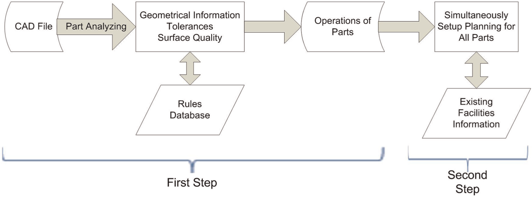
Workflow of information.

Figure 2.

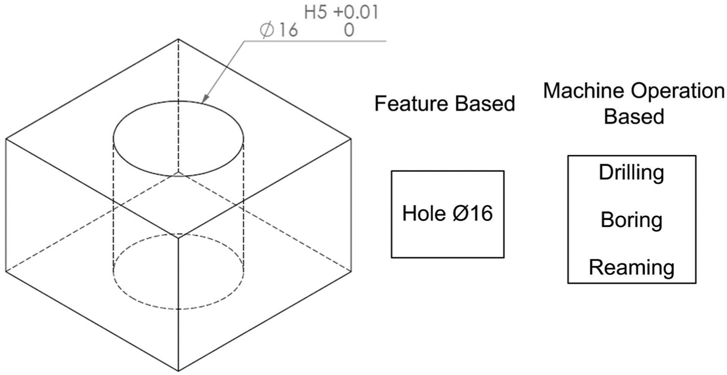
Transformation of feature to machine operation.

The proposed setup planning system clusters, sorts and sequences the machining operations based on some constraints to generate the best process plan with the available resources. These constraints make the operation constraint and precedence (OCP) matrix determine what operations can be grouped into one cluster and precedence between the operations. Operations in the same cluster can be machined in one three-axis-based setup. Some of these constraints must necessarily be carried out, which are mentioned as a strong constraint and some of these are preferred constraints which are mentioned as a weak constraint. If two operations have a weak constraint, they can be grouped in the same setup or not. This enhances the flexibility of the setup plan significantly. This procedure is done for all parts and is saved to restore the production time. At the production time, all operations of parts are distributed among the available resources simultaneously to optimize the objective function which includes the weighted sum of scheduling objectives similar to makespan and the technical objectives such as locating stability.

One of the constraints for assignment of operations into one cluster is the consideration of the TAD. A TAD is a path along which the tool can approach the feature without an obstacle. For a prismatic part, there are six primary TAD directions (±x, ±y, ±z). Some features may be machined in more than one approach direction. Some features may have an approach direction which is different from the six orthogonal directions. If such features have only one TAD, the machining of such features is more expensive in three-axis machines because they need special fixturing requirements. For four-axis and five-axis machines, this problem is not so important because these directions can be achieved by rotation of the table. For features with more than one TAD direction, the TADs that are not in six orthogonal directions have been eliminated. If two operations have the same TAD direction, they would have a weak constraint relationship.

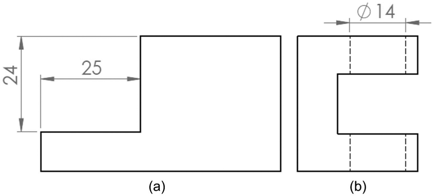
The tolerance relations between features include geometrical and dimensional tolerances. Some geometrical tolerances such as orientation, run out, location and some feature profiles are specified between one target feature and one or more datum features (Figure 3(a)). To avoid or minimize the machining error stack-up, one of the straightforward rules is trying the machine features following their datum dependency precedence if they have a direct datum reference relationship, especially when this relationship is critical. ²³ The other types of geometrical tolerances such as circularity do not have datum and are related to a single feature (Figure 3(b)). Dimensional tolerances are divided into two types of dimensional tolerances: tolerances that are related to two features (Figure 4(a)) or tolerances that are related to one feature (Figure 4(b)).

Figure 3.

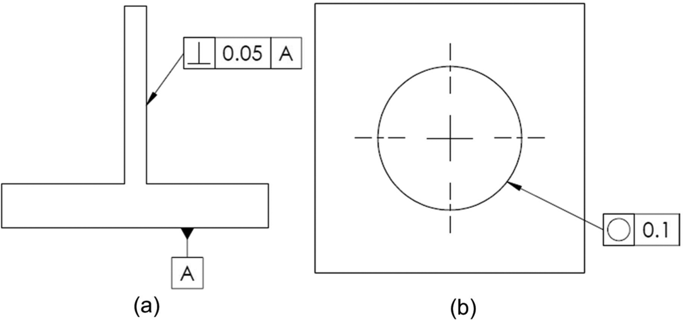
Two types of geometrical tolerances: (a) tolerance related to more than one feature and (b) single-feature tolerance.

Figure 4.

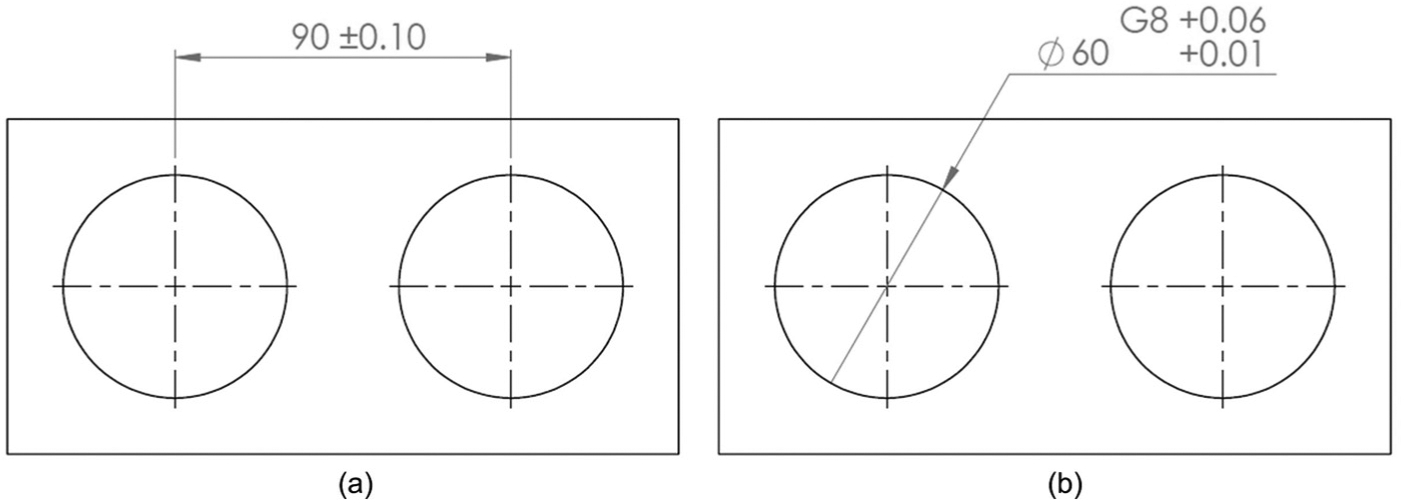
Two types of dimensional tolerances: (a) tolerance related to more than one feature and (b) single-feature tolerance.

In numerical control (NC) machining, three setup methods are used to obtain the dimension between two features. These methods are as follows:

1. Machining the two features in the same setup, where setup error is not included and mainly depends on the machine tool accuracy. The error of the single-feature tolerance is similar.

2. Using one feature as the locating datum and machining the other, in which setup error is added to the machine tool error.

3. Using an intermediate locating datum to machine two features in different setups which is the least desired setup method because for all dimensions obtained using this method, a tolerance chain is formed.

In most of the previous works, the main goal was avoiding setup method 3 and the single-feature tolerance (dimensional and geometrical) is screened out, while this tolerance is one of the most important parameters in selection of the machine tool. Therefore, in addition to the grouping of operations with tight tolerance (dimensional or geometrical) in the same setup as a strong constraint, the tolerance of single features is used to select a proper machine tool.

The other effect of tolerances and surface finish quality is on the operation planning. For example, a hole with tight tolerance in diameter or good surface finish must be complete with extra operations such as boring and reaming. Some of these operations must be executed on one machine and in one setup which is considered as a strong constraint, and if these operations can be executed on different machines, it is considered as a weak constraint. This effect was seldom considered in previous researches.

Another important constraint is good manufacturing practices which are represented as rules of thumb. Some of these practices are important in selection of the best TAD, therefore leading to selection of the proper setup. For example, the best TAD for a setup is normal to the largest surface of the setup, while these rules are not absolutely true especially when two surface areas are near (Figure 5(a)). The other practices are related to the sequence of features in the same setup. For example, if a hole is cut through the other features, the hole drilling should be first (Figure 5(b)). All these rules of thumbs are analyzed and some of them are regarded as a strong constraint and the others are regarded as a weak constraint.

Figure 5.

Examples of manufacturing practice constraint: (a) best TAD selection and (b) priority of operations.

Generate OCP matrix

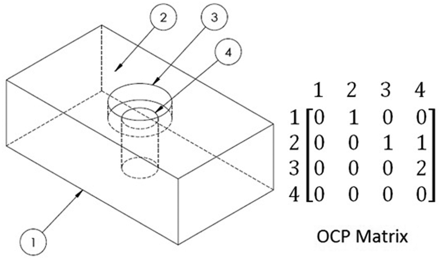
The first step for setup generation is analysis of parts for determining the proper operation. The result of these analyses is stored in the OCP matrix which is an n × n matrix, in which n is the number of operations of the part.

The entry OCP_ijk is defined as follows

$$\mathrm{OC}{P}_{\mathrm{ijk}}=\{\begin{array}{c}1\mathrm{if}\mathrm{operation}j\mathrm{and}k\mathrm{have}a\mathrm{weak}\mathrm{constraint}\mathrm{for}\hfill \\ \multicolumn{1}{c}{\mathrm{part}i\mathrm{and}\mathrm{operation}j}\\ \multicolumn{1}{c}{\mathrm{must}\mathrm{be}\mathrm{executed}\mathrm{before}\mathrm{operation}k\mathrm{or}\mathrm{there}\mathrm{are}}\\ \multicolumn{1}{c}{\mathrm{no}\mathrm{precedence}\mathrm{relation}}\\ \multicolumn{1}{c}{2\mathrm{if}\mathrm{operation}j\mathrm{and}k\mathrm{have}a\mathrm{strong}\mathrm{constraint}}\\ \multicolumn{1}{c}{\mathrm{for}\mathrm{part}i\mathrm{and}\mathrm{operation}j}\\ \multicolumn{1}{c}{\mathrm{must}\mathrm{be}\mathrm{executed}\mathrm{before}\mathrm{operation}k\mathrm{or}}\\ \multicolumn{1}{c}{\mathrm{there}\mathrm{are}\mathrm{no}\mathrm{precedence}\mathrm{relation}}\\ \multicolumn{1}{c}{0\mathrm{otherwise}}\end{array}$$

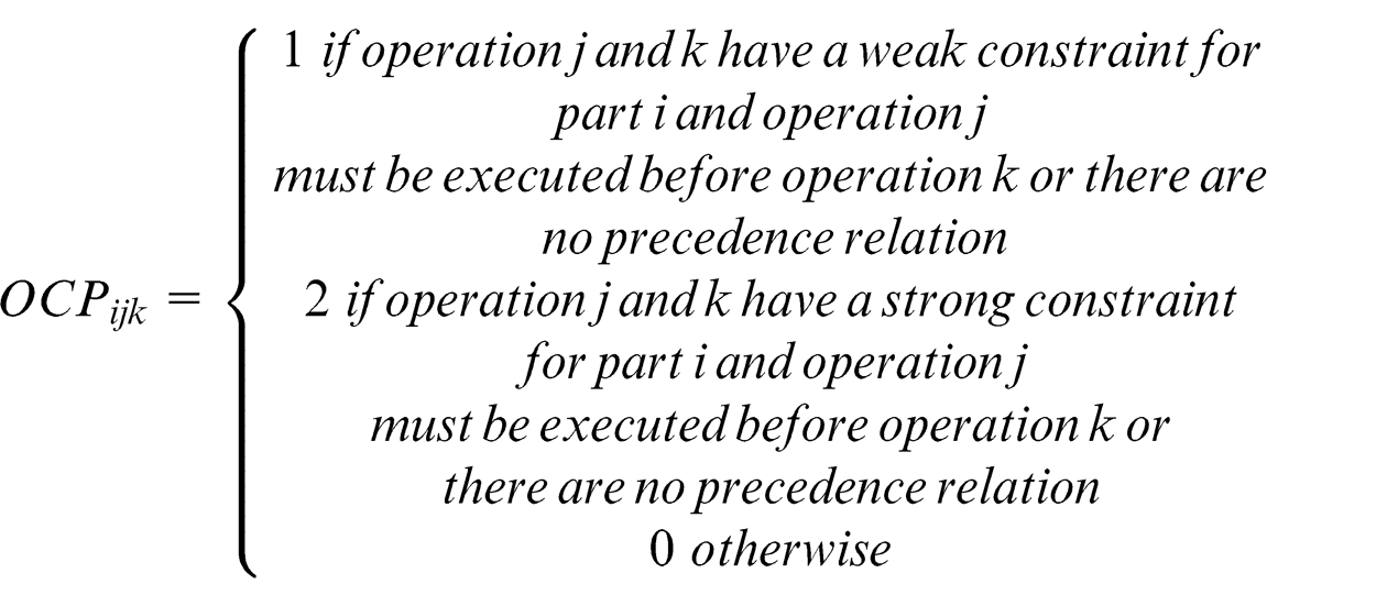
Therefore, if operations j and k have a weak constraint and there are no precedence relations between them OCP_ijk  = OCP_{ik j} = 1. But if operation j must be executed before operation k, OCP_ijk  = 1, OCP_ikj  = 0. This also holds for the operations with a strong constraint.

For filling this matrix, the weak constraints are considered at first and the strong constraints are considered afterward. Therefore, if operations j and k both have weak and strong constraints, the strong constraint is considered. The remaining elements of the matrix are filled with 0. After the constraint and precedence matrix is completely constructed, the groups’ operations are chosen. The groups’ operations are a set of operations which have strong constraints. The remaining operations are considered as a single operation. This partitioning enhances the flexibility of the setup planning.

Proposed algorithm

The general algorithm proposed in this article is presented in Figure 6.

Figure 6.

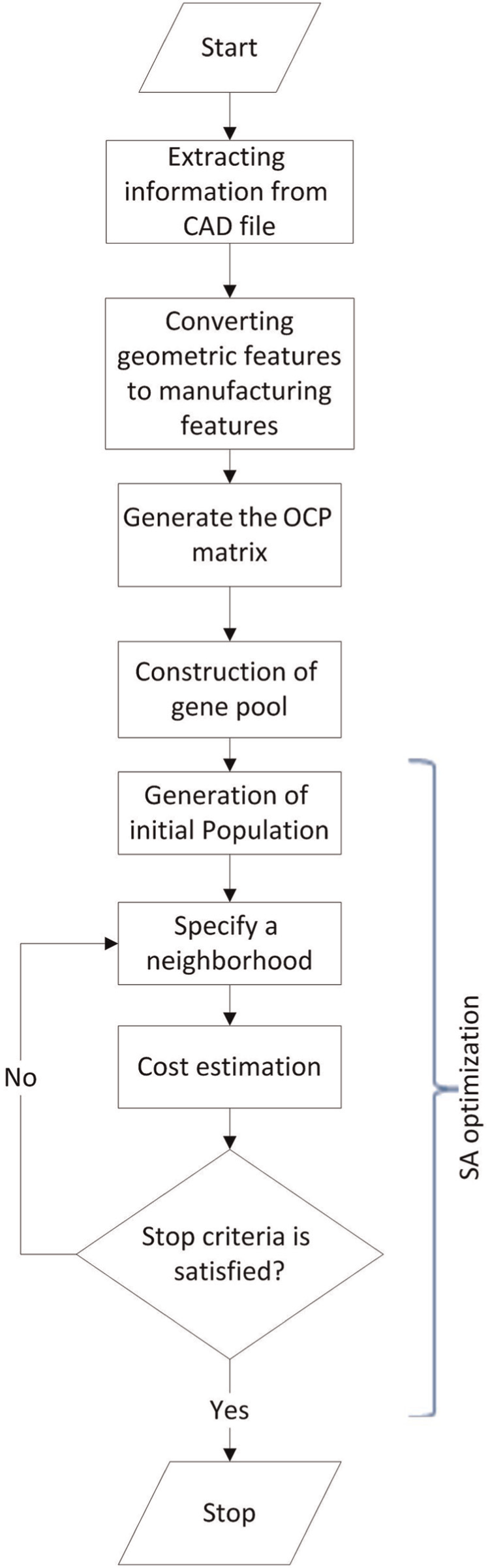
General algorithm.

After essential information is extracted from the CAD file, features are transformed to the operations and the OCP matrix is formed. Using the OCP matrix, operations are classified based on the three-axis setup. Then comes the optimization, in which gene pool generation is the first step. Genes in the pool, including single operations and group operations according to the three-axis-based setup, are shown in Figure 7. Moreover, in the features’ specification, every gene contains information about TADs and machines which have the capability to produce the most accurate features in the group.

Figure 7.

An example of gene.

There are specific pools for each part that have a primary and secondary section. Operations in which their respective columns are 0 are placed in the primary section and the rest are placed in the secondary section. For example, in Figure 8, milling of surface 1 is placed in the primary section and the other operations are placed in the secondary section. If all elements of a column are 0, this ensures that no operation should be performed before this operation.

Figure 8.

An example for primary and secondary section.

SA optimization

An SA is a stochastic searching algorithm which consists of five major processes for integrated process planning and scheduling ¹⁰ :

1. Decide an initial schedule.

2. The initial schedule is chosen as the current schedule.

3. Determine the start temperature (T ₀), the end temperature (T ₁) and setting the start temperature as the current temperature (T = T ₀).

4. While not yet frozen, generate a temporary schedule by neighborhood strategies and then the performance is evaluated and the current temperature decreases.

5. If frozen, the algorithm is ended.

These processes are as follows:

The initial population must be a set of random feasible solutions. For this purpose, a pool of parts is randomly selected and from its primary section, a gene is selected. A machine and TAD are randomly selected for this gene. Rows and the columns related to this gene are removed from the OCP matrix and the genes in the secondary section are searched to find the genes that have the conditions to be transferred to the primary section. This procedure is repeated until all the pools become empty. Selected operations are assigned to the available resources sequentially, then if two operations of a part are on a machine successively, search whether there is the possibility of merging those in which case the common primary locating surface is chosen; otherwise a locating surface is randomly chosen for each. For four-axis and five-axis machines, the merging of different setups is done using the ASP approach that was proposed by Cai et al. ²⁰ This approach searches a primary locating surface for different setups which have the common tool orientation space. Applying this algorithm leads to generating a feasible random solution (Figure 9). This feasible solution is chosen as the current schedule and then the start and end temperatures are chosen.

Figure 9.

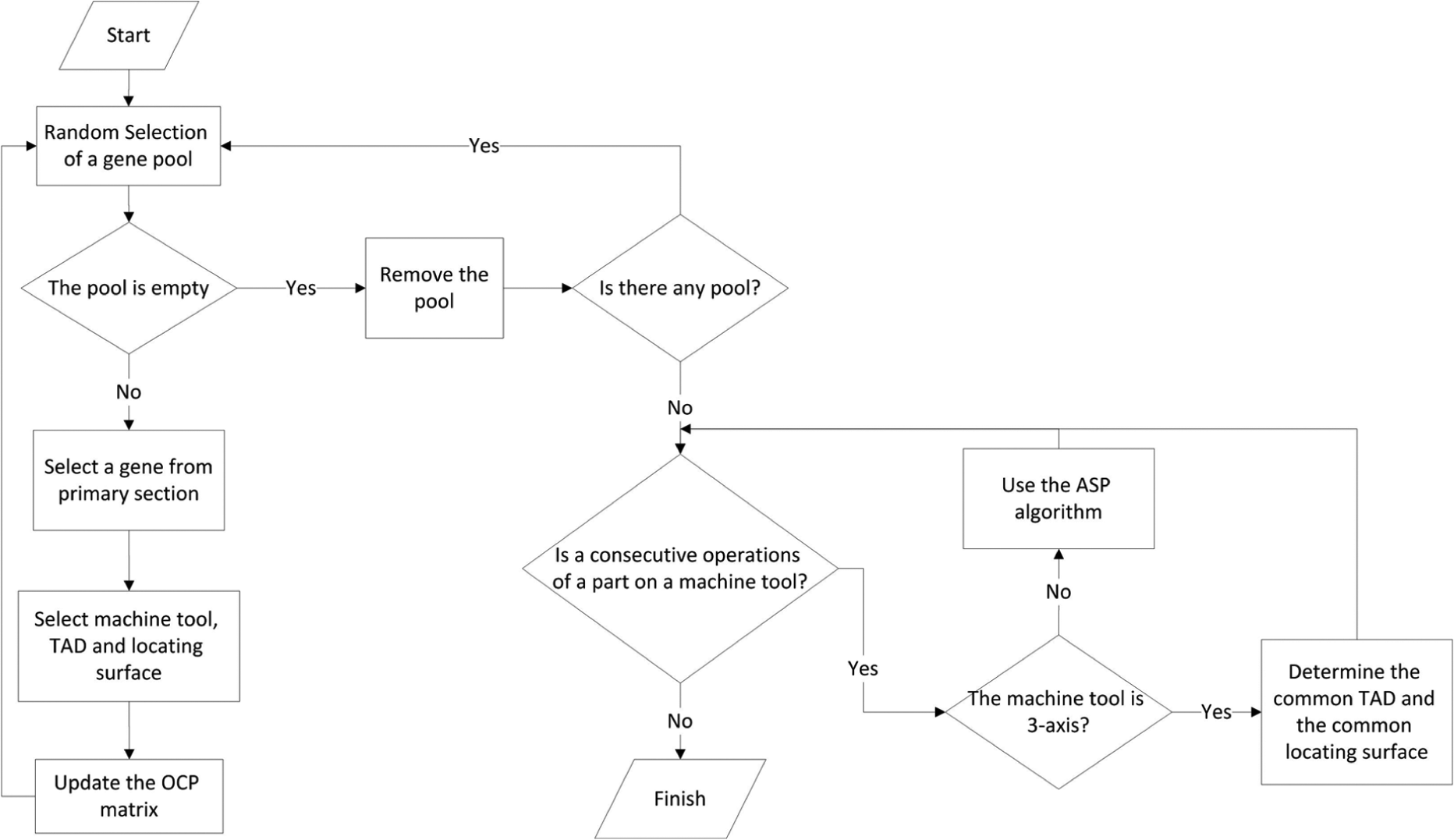
Flowchart of random feasible solution generation.

The neighborhood strategies are explained in three ways:

1. Two groups or single operations can exchange their order in a chromosome if according to the OCP matrix their priority is respected (Figure 10(a)).

2. The machine that is assigned for specific operations can be changed or the primary locating surface can also be changed (Figure 10(b)).

3. If two groups’ operations are not in the neighborhood of the other and have the conditions to merge, these operations come together and are merged. The reverse of this procedure is also possible, which is called decomposition (Figure 10(c)).

Figure 10.

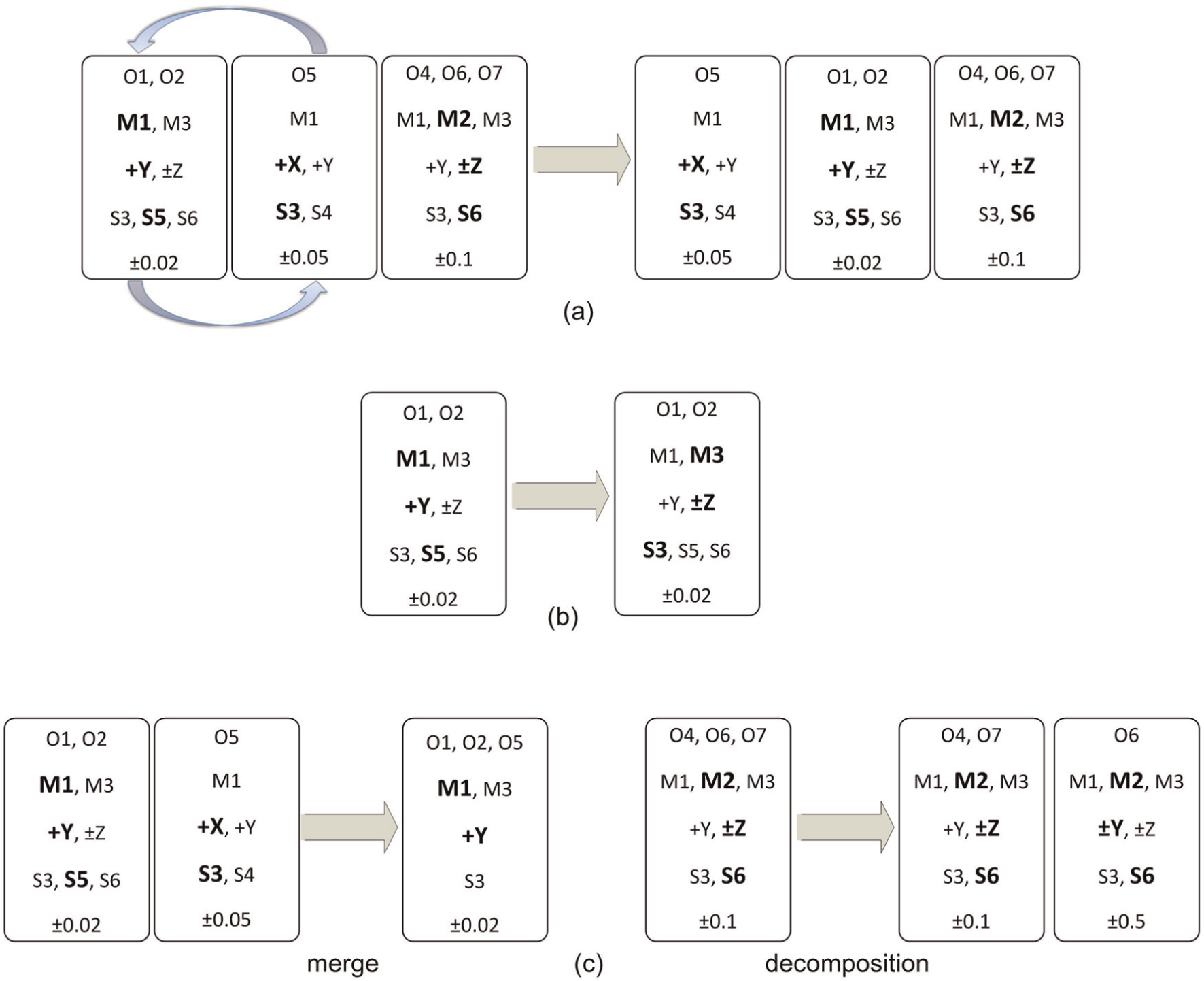
Types of neighborhood in SA: (a) order exchange, (b) parameters’ change and (c) merge and decomposition.

For performance evaluation, an objective function is used in this article. This objective function is the weighted sum of locating surface stability, setup number, machining cost, makespan and machine utilization, the first three criteria of which are technical objectives and the last two are scheduling criteria

$$\begin{array}{c}\multicolumn{1}{c}{\mathrm{objective}\mathrm{function}=\max \frac{1}{P}{\displaystyle \sum _{p=1}^P}(w_l\times L{F}_p+w_G\times G{F}_p}\\ \multicolumn{1}{c}{+w_c\times C{F}_p+w_m\times M{F}_p+w_u\times {\mathrm{UF}}_p)}\end{array}$$

(1)

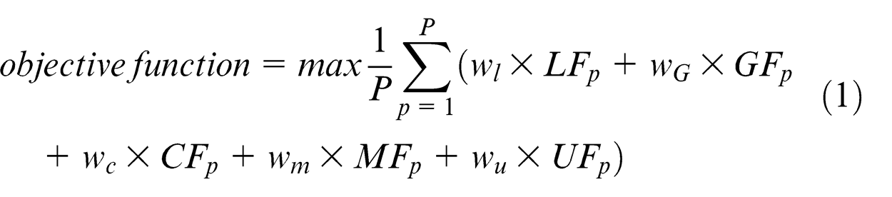
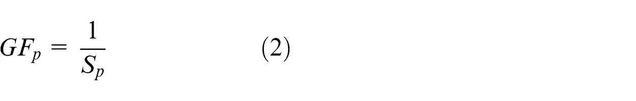
where w_l, w_g, w_c, w_m and w_u are weights of locating factor, grouping factor, cost factor, makespan factor and utilization factor, respectively, and p is the number of the part. LF_p is the locating factor that evaluates the quality of locating surface, and the articles of Wang et al. ⁴ and Mohapatra et al. ⁵ presented a detailed discussion about how it is calculated. GF_p is a grouping factor that is used to minimize the number of setups and is calculated as follows

$$G{F}_p=\frac{1}{S_p}$$

(2)

where S_p is the number of setups for part p. CF_p is the cost factor and is calculated by

$$C{F}_p=\frac{{\displaystyle \sum _{s=1}^{S_p}}{\displaystyle \sum _{f=1}^{Q_p^s}}M{T}_f\times {\mathrm{UC}}_p^{\mathrm{cheap}}}{{\displaystyle \sum _{s=1}^{S_p}}{\displaystyle \sum _{f=1}^{Q_p^s}}M{T}_f\times {\mathrm{UC}}_p^s}$$

(3)

where $Q_p^s$ is the number of machining feature in setup s, MT_f is the machining time of feature f, ${\mathrm{UC}}_p^s$ is the unit cost of the machine which is used for setup s and ${\mathrm{UC}}_p^{\mathrm{cheap}}$ is the unit cost on a low-end machine with a cheap unit cost. MF_p is a makespan factor that is calculated as follows

$$M{F}_p=\frac{M{S}_{{\min }_p}}{M{S}_p}$$

(4)

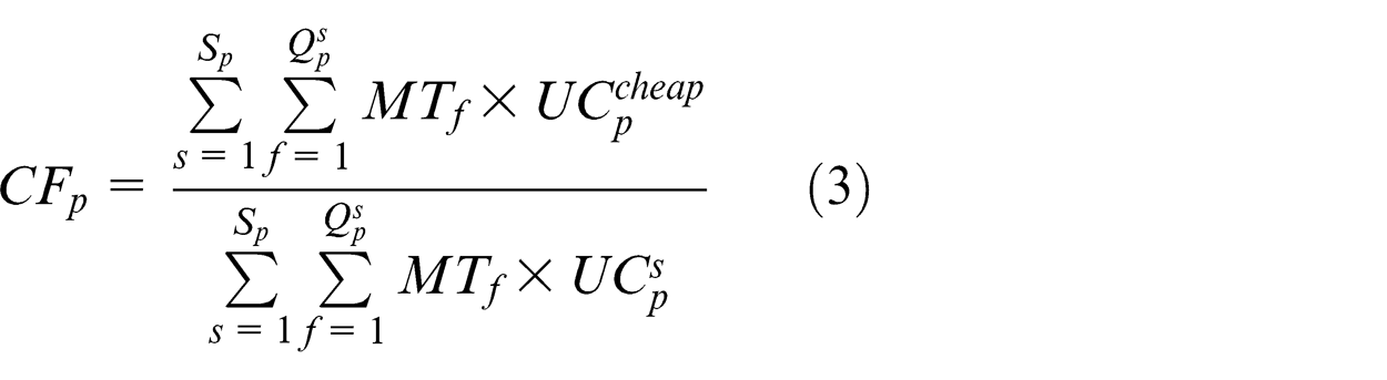
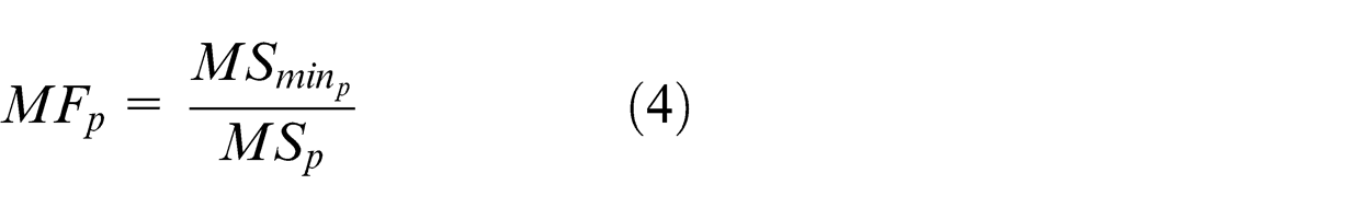
where MS_p is the makespan and is equivalent to when the last operation of each part is completed and $M{S}_{{\min }_p}$ is calculated as follows

$$M{S}_{\min }={\displaystyle \sum _{s=1}^{S_p}}{\displaystyle \sum _{f=1}^{Q_p^s}}M{T}_f$$

(5)

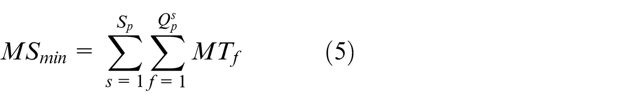
This means that all parts of the operations are to be performed sequentially without any delay. In the articles that have been published in this field, such as Mohapatra et al., ⁵ MS_p is calculated by adding a constant value that is non-machining time, but this assumption is not at all true especially when there are multiparts, and the waiting time is very different for each part and every setup. In this article, the exact makespan is calculated.

The current temperature is updated as follows

$$T=\alpha \times T$$

(6)

where 0 < α < 1.

Finally, the frozen criteria are checked (T ≤ T ₁), if so the algorithm ends.

Illustrative example

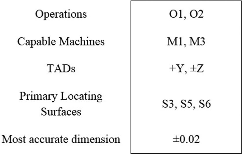
The part that is chosen for describing the algorithm procedure is depicted in Figure 11. The feature specifications are described in Table 1, and the machine tool specification is reported in Table 2. This part consists of eight features. For the groups’ operation, a common TAD is selected. This TAD is mentioned as the constrained TAD and is shown in the last column in Table 1. For example, the face milling of feature 1 and drilling of feature 4 must be executed in the same setup; therefore, the TAD direction of these features is reduced to +z. This is a significantly reduced search space. The OCP matrix is shown in Figure 12. It should be considered that in the first OCP matrix if two operations have a common TAD and the proposed machines, they could have a weak constraint. By selection of machine tools for each operation, the OCP matrix is updated. For example, if M1 is selected for operation 9, it could not be merged with operation 3, because M1 is not proper for operation 3 and therefore OCP (3, 9) and OCP (9, 3) become 0. For simplicity, a unit time is assigned for performing all operations and five unit times for changing setups or machines.

Figure 11.

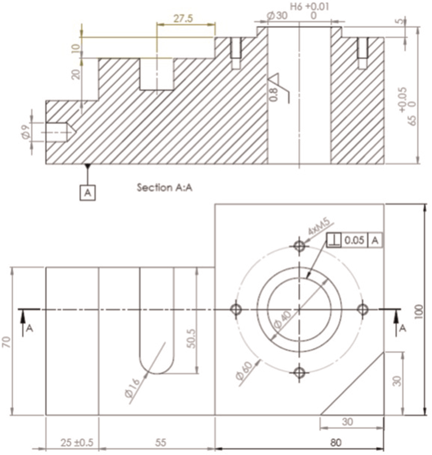
First example.

Table 1.

Feature specification.

Feature no.	Operation no.	TAD directions	Accuracy	Proposed machines	Constrained TAD
Face (1)	Op1: face milling	±x, ±y, +z	General	M2, M3, M4	+z
Step (2)	Op2: face milling	±x, ±y, −z	0.5	M2, M3, M4	+y
Slot (3)	Op3: slot milling	−z	General	M2, M3, M4	−z
Through hole (4)	Op4: drilling	±z	General	M1, M2, M3, M4	+z
	Op5: boring	±z	0.01	M4, M5	±z
	Op6: reaming	±z	0.01	M4, M5	±z
Boss (5)	Op7: rough milling	−z	General	M2, M3, M4	−z
	Op8: finish milling	−z	0.05	M2, M3, M4	−z
Tapped hole (6)	Op9: drilling	−z	General	M1, M2, M3, M4	−z
	Op10: tapping	−z	General	M1, M2, M3, M4	−z
Corner notch (7)	Op11: milling	−z, a	General	M2, M3, M4	−z
Blind hole (8)	Op12: drilling	+y	General	M1, M2, M3, M4	+y

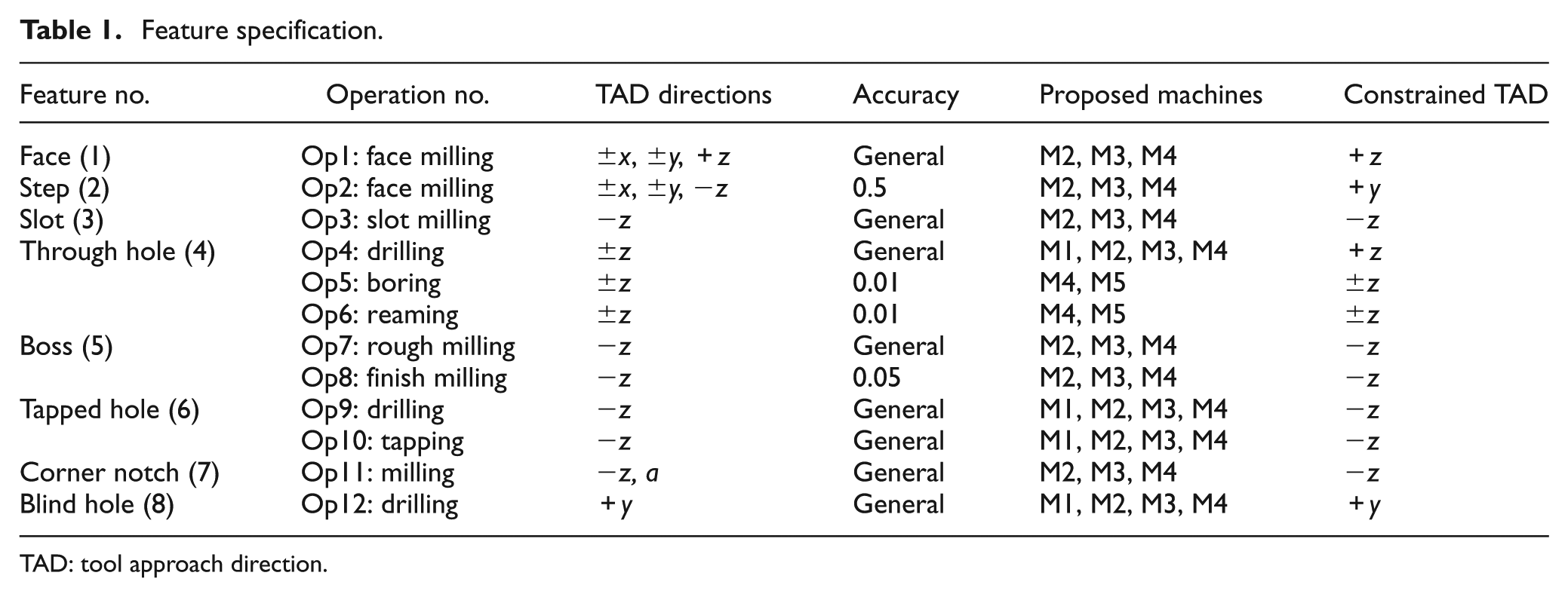
TAD: tool approach direction.

Table 2.

Machine tool’s specification.

Machine no.	Specification	Machining cost/time	Accuracy
M1	Drilling machine	10	0.1
M2	CNC milling machine (three-axis)	30	0.05
M3	CNC milling machine (four-axis)	50	0.01
M4	CNC milling machine (three-axis)	80	0.005
M5	Boring machine	40	0.01

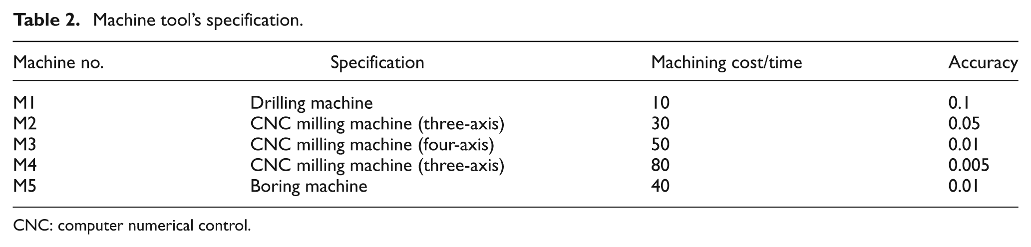
CNC: computer numerical control.

Figure 12.

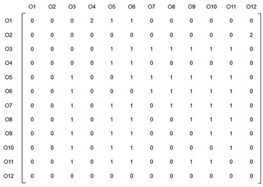
Primary feature precedence constraint matrix.

The objective function, which is expressed in equation (1), includes locating factor, grouping factor, cost factor, makespan factor and machine utilization factor in which different scenarios are examined by their weights and are given in Table 3. To execute all experiments, a laptop with Core i5 processor and 4 GB RAM is used.

Table 3.

Different scenarios.

Scenario no.	Weights	Objective
1	Wl  = Wg  = 1 Wc  = Wm  = Wu  = 0	To utilize the most capable machines
2	Wl  = Wg  = Wc  = 1 Wm  = Wu  = 0	To reduce cost and setup simultaneously
3	Wl  = Wg  = Wm  = 1 Wc  = Wu  = 0	To reduce makespan regardless of cost
4	Wl  = Wg  = Wc  = Wm  = Wu  = 1	A trade-off between all criteria
5	Wl  = Wg  = 1 Wc  = 2 Wm  = Wu  = 0	To reduce cost as much as possible

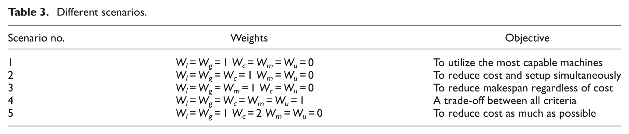
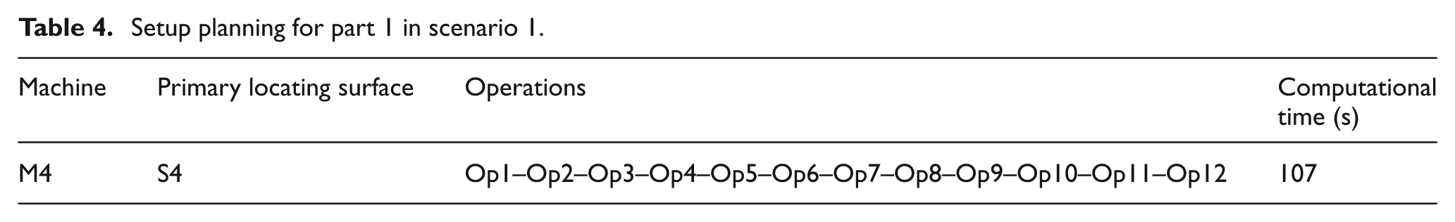
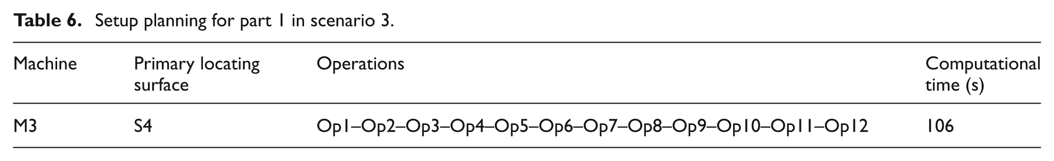
In the first scenario, when only a technological constraint is an issue, only the M4 machine is used which is able to perform all operations in a setup to increase the grouping factor. The biggest surface is also selected to increase the locating factor (Table 4). In the second scenario, when the cost issue is also raised, M4 is replaced by M3 which also has the ability to perform all operations in a setup with a lower cost (Table 5). In the third scenario, the cost factor is replaced by the makespan factor so M3 is selected again to perform all operations until no time is spent for changing setups or machines and the lowest makespan is achieved (Table 6).

Table 4.

Setup planning for part 1 in scenario 1.

Machine	Primary locating surface	Operations	Computational time (s)
M4	S4	Op1–Op2–Op3–Op4–Op5–Op6–Op7–Op8–Op9–Op10–Op11–Op12	107

Table 5.

Setup planning for part 1 in scenario 2.

Machine	Primary locating surface	Operations	Computational time (s)
M3	S4	Op1–Op2–Op3–Op4–Op5–Op6–Op7–Op8–Op9–Op10–Op11–Op12	106

Table 6.

Setup planning for part 1 in scenario 3.

Machine	Primary locating surface	Operations	Computational time (s)
M3	S4	Op1–Op2–Op3–Op4–Op5–Op6–Op7–Op8–Op9–Op10–Op11–Op12	106

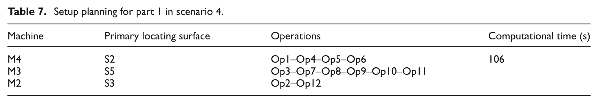
In the fourth scenario, all the objectives have the same weights and all operations are distributed relatively evenly among the three machines. The grouping factor and the makespan factor will prevent the use of M1 and M5 (Table 7).

Table 7.

Setup planning for part 1 in scenario 4.

Machine	Primary locating surface	Operations	Computational time (s)
M4	S2	Op1–Op4–Op5–Op6	106
M3	S5	Op3–Op7–Op8–Op9–Op10–Op11
M2	S3	Op2–Op12

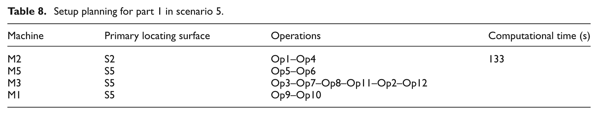
In the latter scenario, the cost has the highest weight; thus, machines M1 and M5, which are for specific processes but have less cost, are used more. For this purpose, M4 machine is not used. The reason for using M3 is the grouping factor (Table 8).

Table 8.

Setup planning for part 1 in scenario 5.

Machine	Primary locating surface	Operations	Computational time (s)
M2	S2	Op1–Op4	133
M5	S5	Op5–Op6
M3	S5	Op3–Op7–Op8–Op11–Op2–Op12
M1	S5	Op9–Op10

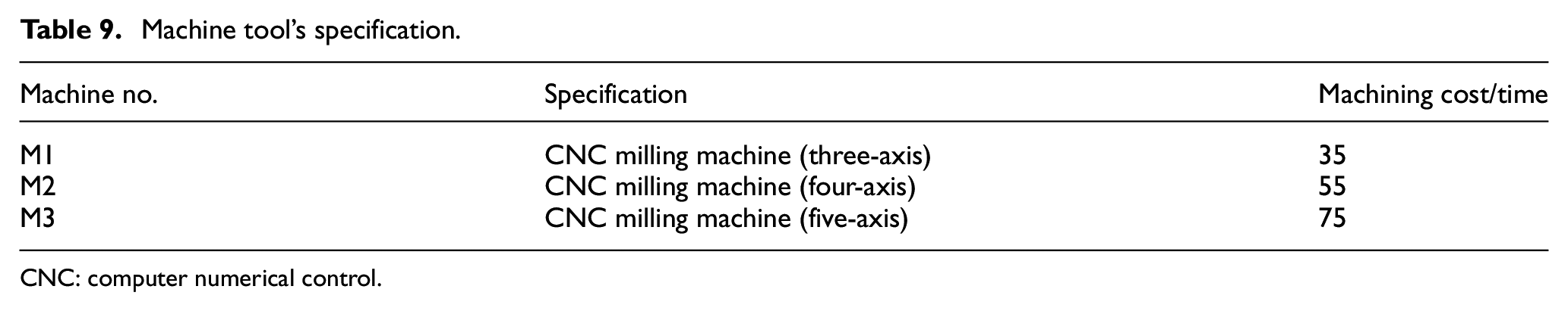
The comprehensive example consists of three parts (Figure 13–15) which are adopted from Mohapatra et al. ⁵ (Appendix 1). All these parts are available at 0 time and must be executed on three machine tools (Table 9). This example is presented to show the effect of multipart setup planning versus single-part setup planning. Five scenarios that are represented in Table 3 are repeated here and the results are compared with AIS-based algorithm ⁵ and genetic algorithm (GA) ²³ for each of the individual parts performed.

Figure 13.

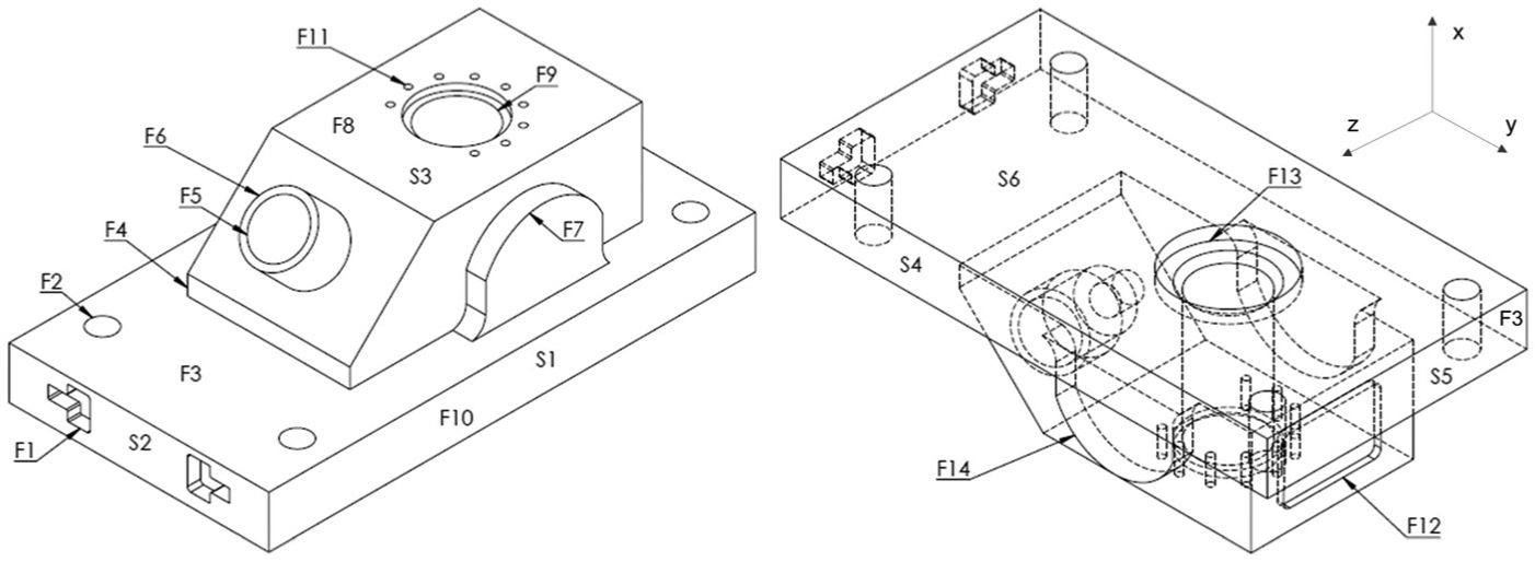
First part of second experiment.

Figure 14.

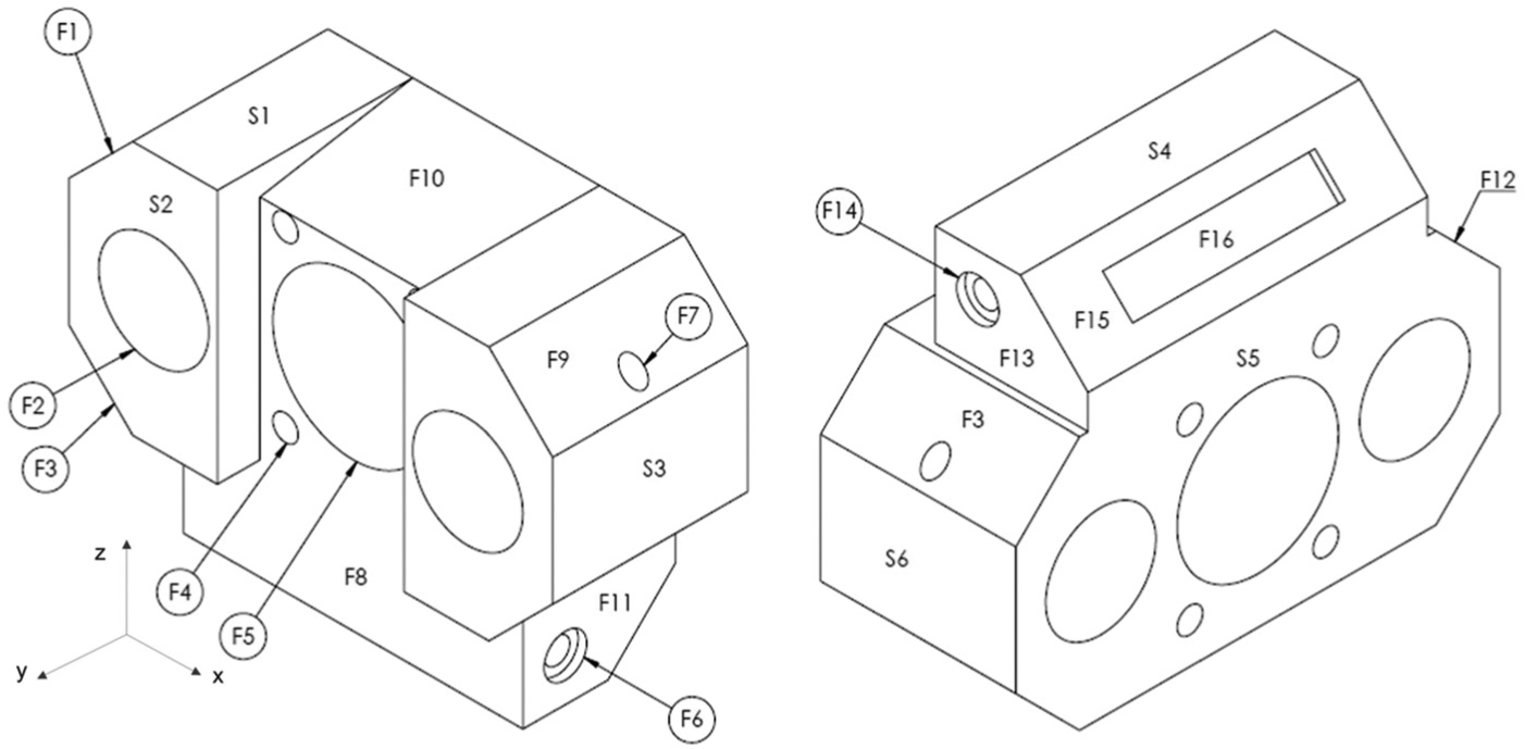
Second part of second experiment.

Figure 15.

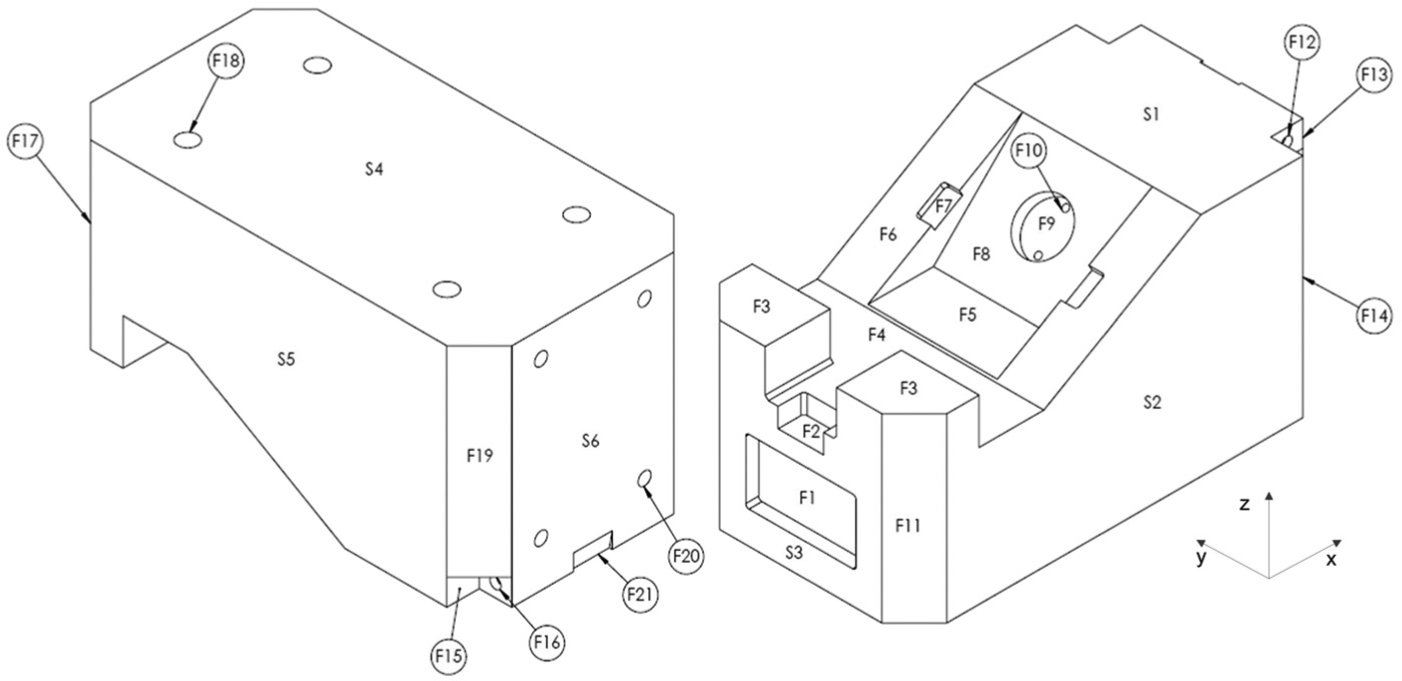
Third part of second experiment.

Table 9.

Machine tool’s specification.

Machine no.	Specification	Machining cost/time
M1	CNC milling machine (three-axis)	35
M2	CNC milling machine (four-axis)	55
M3	CNC milling machine (five-axis)	75

CNC: computer numerical control.

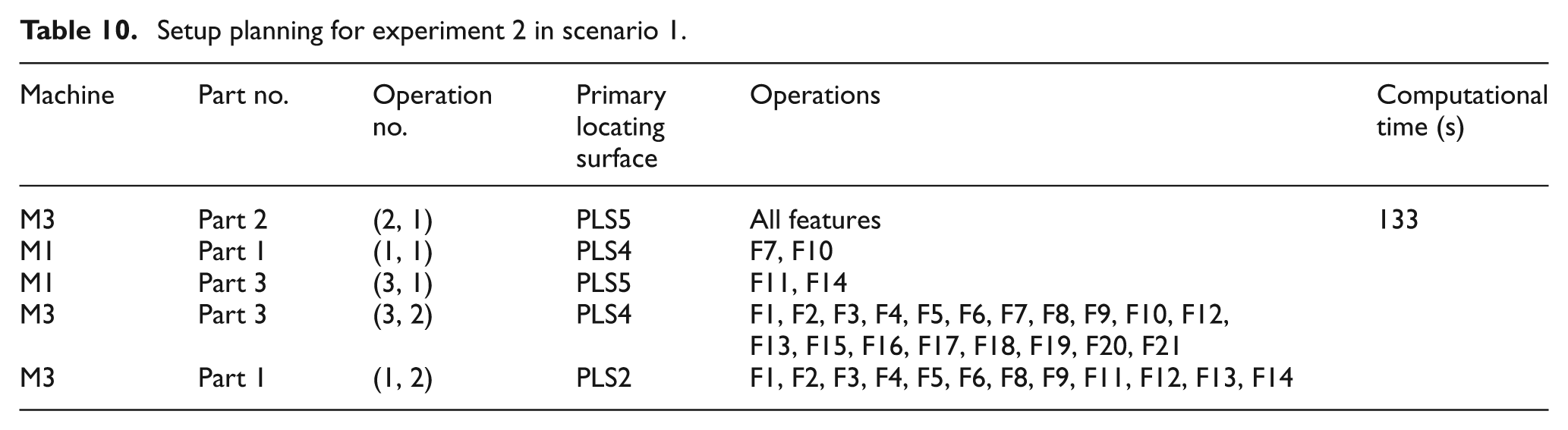
In the first scenario that cost, makespan and the machine utilization have no effects on the results, all operations are executed on M3 which is capable of doing all operations of parts in one setup except some features (F7 and F10 from part 1 and F11 and F14 from part 3) because there is no possibility to generate all features of these two parts in a setup (Table 10). Relevant Gantt chart is shown in Figure 16.

Table 10.

Setup planning for experiment 2 in scenario 1.

Machine	Part no.	Operationno.	Primary locating surface	Operations	Computationaltime (s)
M3	Part 2	(2, 1)	PLS5	All features	133
M1	Part 1	(1, 1)	PLS4	F7, F10
M1	Part 3	(3, 1)	PLS5	F11, F14
M3	Part 3	(3, 2)	PLS4	F1, F2, F3, F4, F5, F6, F7, F8, F9, F10, F12, F13, F15, F16, F17, F18, F19, F20, F21
M3	Part 1	(1, 2)	PLS2	F1, F2, F3, F4, F5, F6, F8, F9, F11, F12, F13, F14

Figure 16.

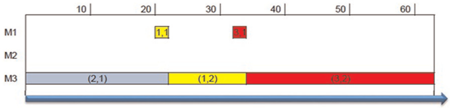
Gantt chart of experiment 2 in scenario 1.

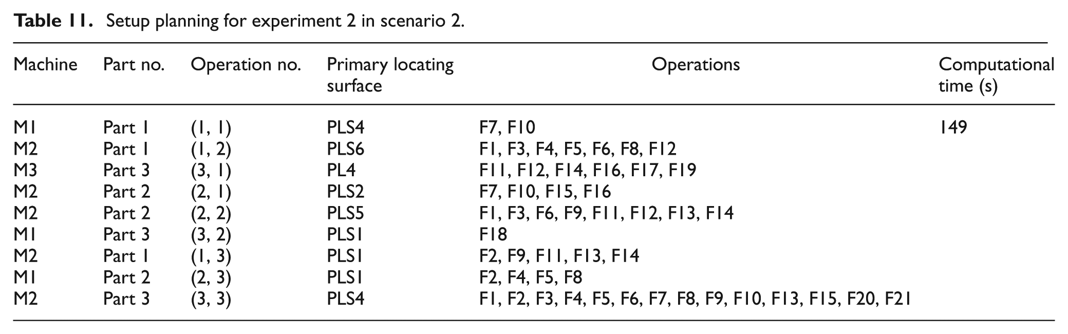
In the second scenario, the cost has to be considered and M3 is replaced by M2 which is less expensive except some operations for part 3. Although the numbers of setups are increased, this increase is compensated by the reduction in cost (Table 11). Relevant Gantt chart is shown in Figure 17.

Table 11.

Setup planning for experiment 2 in scenario 2.

Machine	Part no.	Operation no.	Primary locating surface	Operations	Computational time (s)
M1	Part 1	(1, 1)	PLS4	F7, F10	149
M2	Part 1	(1, 2)	PLS6	F1, F3, F4, F5, F6, F8, F12
M3	Part 3	(3, 1)	PL4	F11, F12, F14, F16, F17, F19
M2	Part 2	(2, 1)	PLS2	F7, F10, F15, F16
M2	Part 2	(2, 2)	PLS5	F1, F3, F6, F9, F11, F12, F13, F14
M1	Part 3	(3, 2)	PLS1	F18
M2	Part 1	(1, 3)	PLS1	F2, F9, F11, F13, F14
M1	Part 2	(2, 3)	PLS1	F2, F4, F5, F8
M2	Part 3	(3, 3)	PLS4	F1, F2, F3, F4, F5, F6, F7, F8, F9, F10, F13, F15, F20, F21

Figure 17.

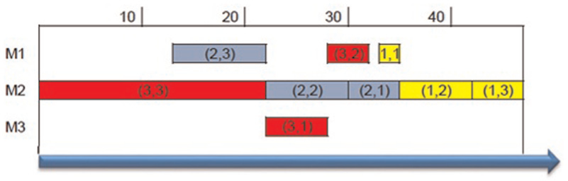
Gantt chart of experiment 2 in scenario 2.

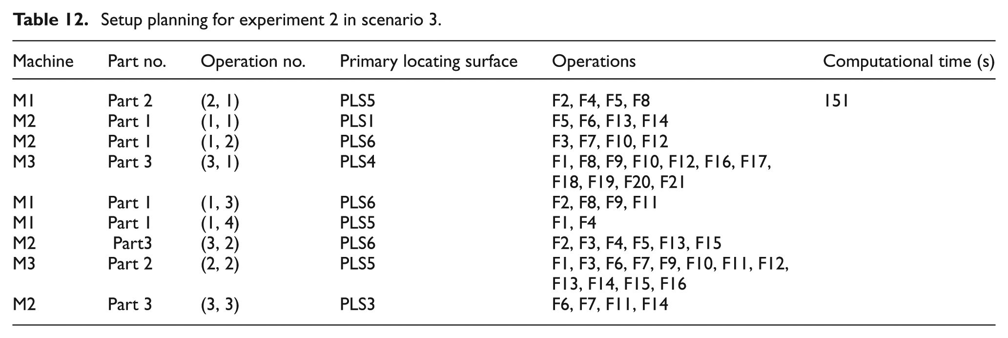
In the third scenario, in which cost is replaced by makespan, operations are more evenly distributed between machines so that the idle time of machines has to be less to have minimum makespan (Table 12). Relevant Gantt chart is shown in Figure 18.

Table 12.

Setup planning for experiment 2 in scenario 3.

Machine	Part no.	Operation no.	Primary locating surface	Operations	Computational time (s)
M1	Part 2	(2, 1)	PLS5	F2, F4, F5, F8	151
M2	Part 1	(1, 1)	PLS1	F5, F6, F13, F14
M2	Part 1	(1, 2)	PLS6	F3, F7, F10, F12
M3	Part 3	(3, 1)	PLS4	F1, F8, F9, F10, F12, F16, F17, F18, F19, F20, F21
M1	Part 1	(1, 3)	PLS6	F2, F8, F9, F11
M1	Part 1	(1, 4)	PLS5	F1, F4
M2	Part3	(3, 2)	PLS6	F2, F3, F4, F5, F13, F15
M3	Part 2	(2, 2)	PLS5	F1, F3, F6, F7, F9, F10, F11, F12, F13, F14, F15, F16
M2	Part 3	(3, 3)	PLS3	F6, F7, F11, F14

Figure 18.

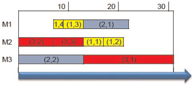
Gantt chart of experiment 2 in scenario 3.

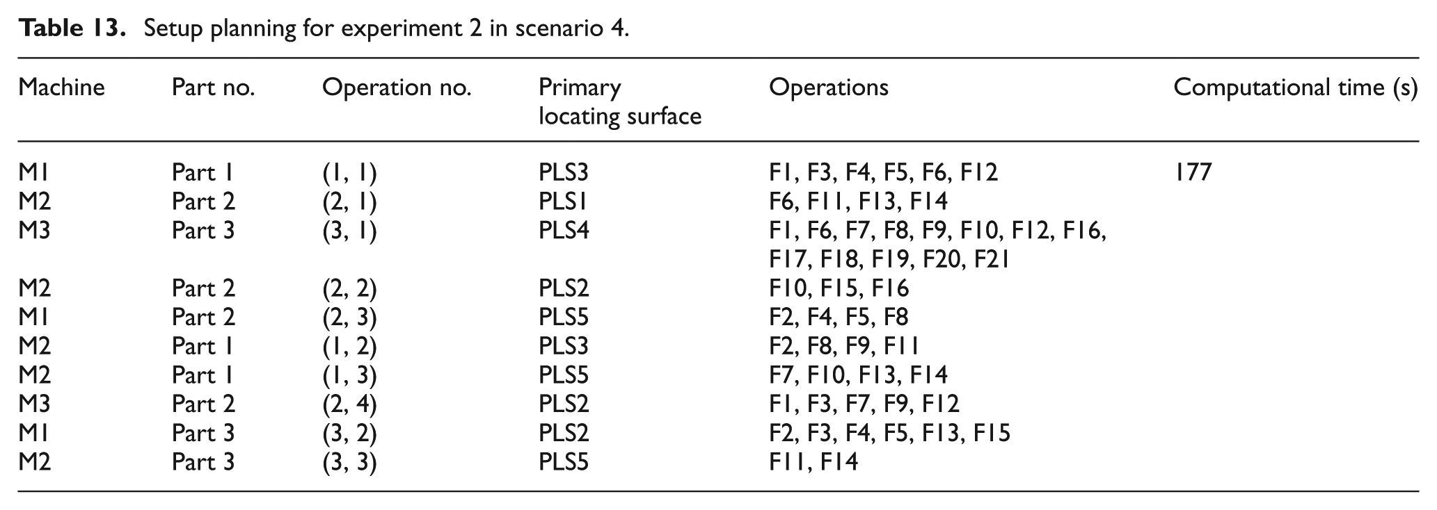
In the fourth scenario, in which all weights are equal, the condition is the same as the previous scenario and operations of all parts are distributed among the three machines (Table 13). Relevant Gantt chart is shown in Figure 19.

Table 13.

Setup planning for experiment 2 in scenario 4.

Machine	Part no.	Operation no.	Primary locating surface	Operations	Computational time (s)
M1	Part 1	(1, 1)	PLS3	F1, F3, F4, F5, F6, F12	177
M2	Part 2	(2, 1)	PLS1	F6, F11, F13, F14
M3	Part 3	(3, 1)	PLS4	F1, F6, F7, F8, F9, F10, F12, F16, F17, F18, F19, F20, F21
M2	Part 2	(2, 2)	PLS2	F10, F15, F16
M1	Part 2	(2, 3)	PLS5	F2, F4, F5, F8
M2	Part 1	(1, 2)	PLS3	F2, F8, F9, F11
M2	Part 1	(1, 3)	PLS5	F7, F10, F13, F14
M3	Part 2	(2, 4)	PLS2	F1, F3, F7, F9, F12
M1	Part 3	(3, 2)	PLS2	F2, F3, F4, F5, F13, F15
M2	Part 3	(3, 3)	PLS5	F11, F14

Figure 19.

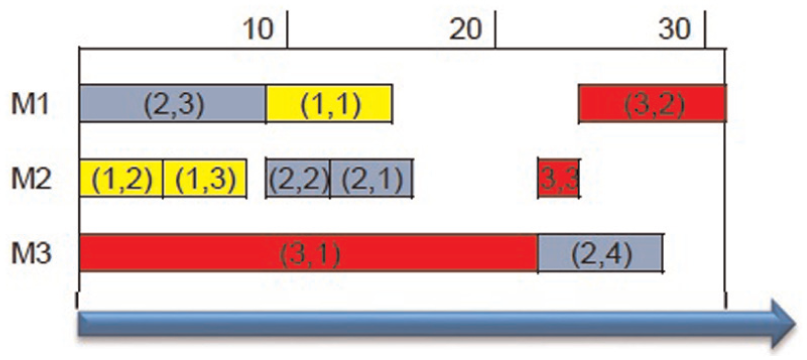
Gantt chart of experiment 2 in scenario 4.

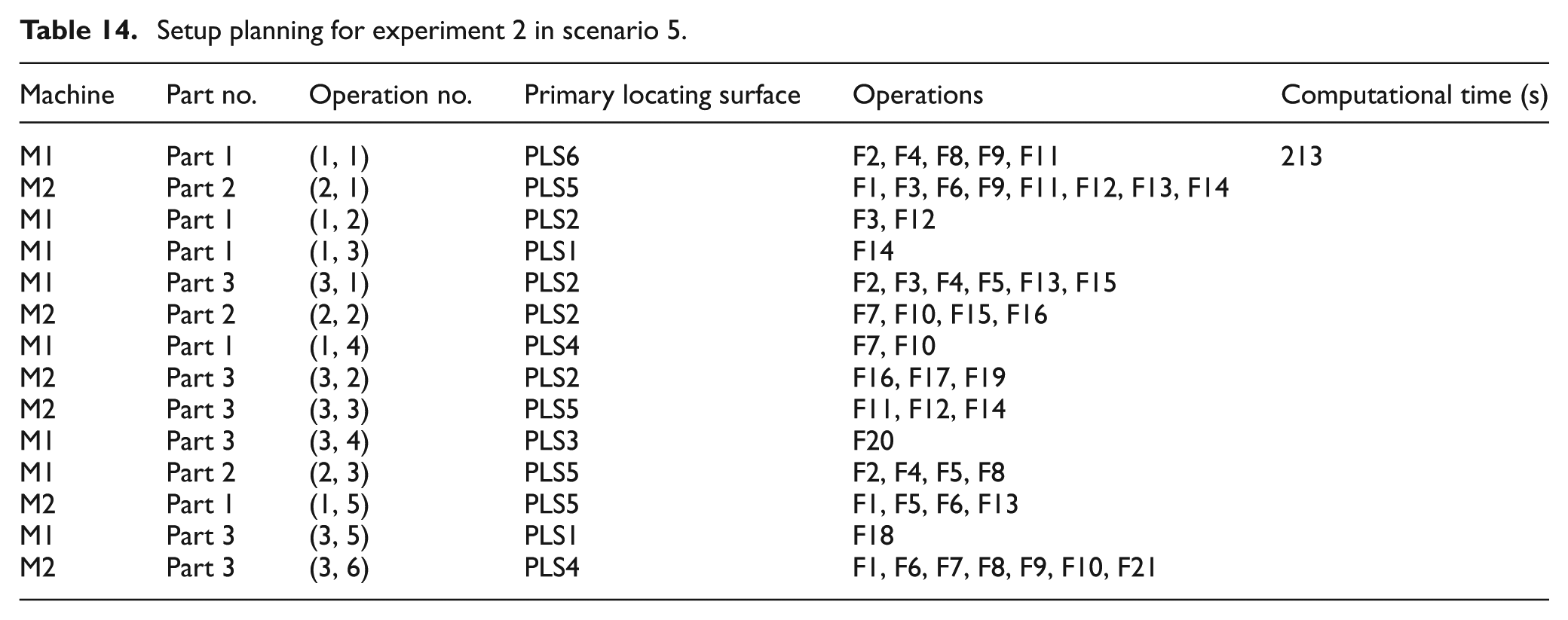
In the last scenario, in which cost has the greatest weight, we observe the increasing use of M1 and M3 is removed (Table 14). Relevant Gantt chart is shown in Figure 20. The overall comparison between the system proposed in this article and AIS ⁵ is presented in Table 15.

Table 14.

Setup planning for experiment 2 in scenario 5.

Machine	Part no.	Operation no.	Primary locating surface	Operations	Computational time (s)
M1	Part 1	(1, 1)	PLS6	F2, F4, F8, F9, F11	213
M2	Part 2	(2, 1)	PLS5	F1, F3, F6, F9, F11, F12, F13, F14
M1	Part 1	(1, 2)	PLS2	F3, F12
M1	Part 1	(1, 3)	PLS1	F14
M1	Part 3	(3, 1)	PLS2	F2, F3, F4, F5, F13, F15
M2	Part 2	(2, 2)	PLS2	F7, F10, F15, F16
M1	Part 1	(1, 4)	PLS4	F7, F10
M2	Part 3	(3, 2)	PLS2	F16, F17, F19
M2	Part 3	(3, 3)	PLS5	F11, F12, F14
M1	Part 3	(3, 4)	PLS3	F20
M1	Part 2	(2, 3)	PLS5	F2, F4, F5, F8
M2	Part 1	(1, 5)	PLS5	F1, F5, F6, F13
M1	Part 3	(3, 5)	PLS1	F18
M2	Part 3	(3, 6)	PLS4	F1, F6, F7, F8, F9, F10, F21

Figure 20.

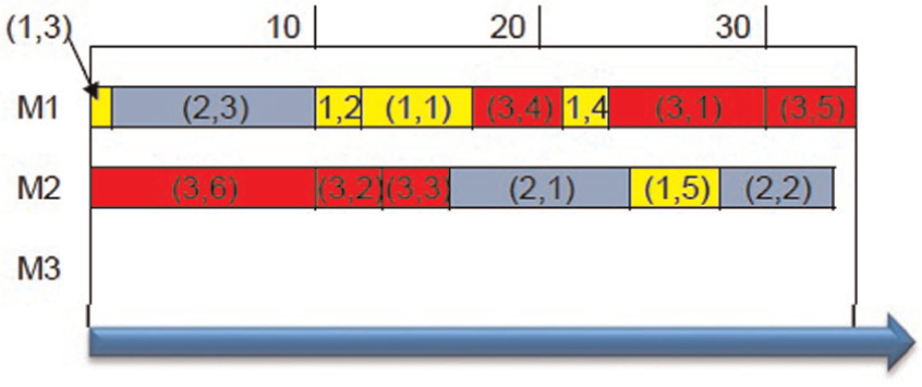
Gantt chart of experiment 2 in scenario 5.

Table 15.

Result of proposed system and AIS.

	GA		AIS		Proposed system
	Objective function	Makespan	Objective function	Makespan	Objective function	Makespan
Scenario 1	1.38	63	1.38	63	1.38	63
Scenario 2	1.66	34	1.77	31	1.83	47
Scenario 3	2.01	31	2.01	31	2.08	31
Scenario 4	3.37	43	3.33	45	3.72	31
Scenario 5	2.43	41	2.44	40	2.54	34

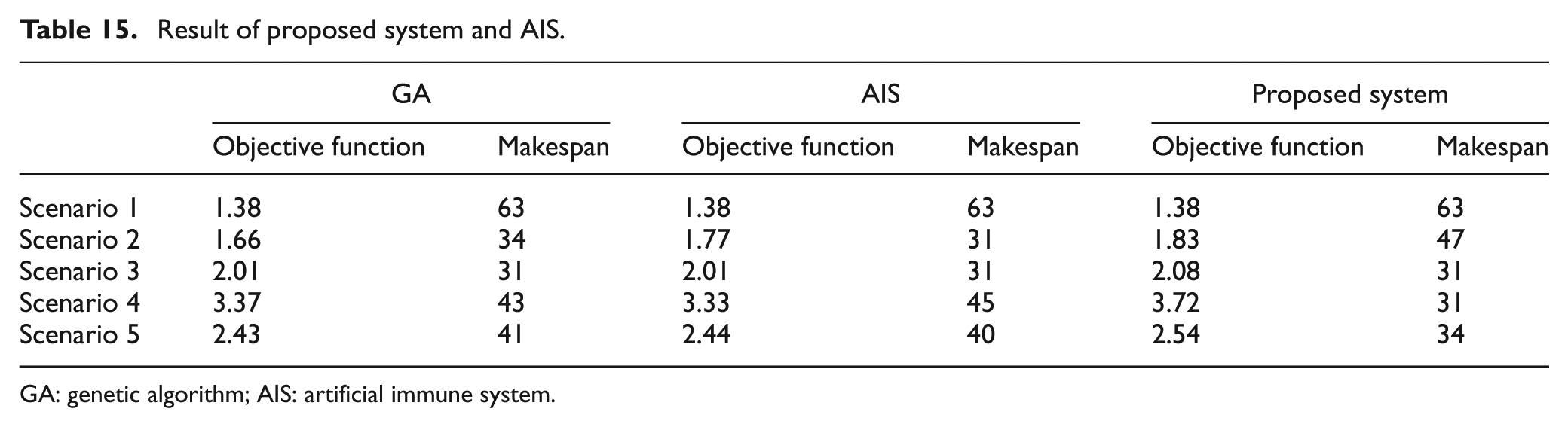
GA: genetic algorithm; AIS: artificial immune system.

The results of the first, second and third scenarios are relatively similar to AIS results. ⁵ In the fourth scenario, using the results of AIS ⁵ greatly increases the cost and time. In the fourth scenario, if setup planning for each part is done separately and these results are then combined, the makespan increases by 31%. This is because setup planning for each part is done individually and regardless of the situation of other parts. In the latter scenario, the results are similar once more. In almost all scenarios, the results of the proposed algorithm of the GA are superior. The interesting point here is that in the fourth scenario, the results of the AIS are superior to the GA for the individual parts, ⁵ but in the multipart setup planning situation the results of the GA are better.

As the results show, the greatest effect of integration for multipart is for scenario 4 in which the makespan greatly changes. Of course if for cost estimation, in addition to the machining cost, the cost of storage and the penalty of delay are also considered; the cost would be significantly changed.

Conclusion

In this article, a new approach for setup planning of multiparts is presented, with the IPPS. It first extracts data from the CAD file and transfers feature data to machining operation. Then the OCP matrix is built to specify what operations can be grouped into one cluster and precedence between the operations. This clustering is based on the strong (necessary) constraint and weak (preferred) constraint which includes the technological and production environment necessities. The pool that consists of operation specifications is built based on this matrix for every part. The SA is used to generate a feasible solution with data which are in pools. This procedure is done for all parts and is saved while in the production time, and all operations of the parts are distributed among the available resources simultaneously to optimize the weighted sum of scheduling objectives and the technical objectives. In this procedure, tolerances are considered in the feature for operation transfer, in machine selection and in the OCP matrix to show the relation and precedence between operations. The results show that the main effect of the proposed system is on the scheduling objectives such as makespan and machining cost.

The contribution of this article can be summarized as follows:

1. The setup planning is done for multiparts simultaneously.

2. Consideration of tolerances for the single feature and two features in different steps of setup planning.