
Abstract
One of the main objectives of computer-aided process planning is to determine the optimum machining sequences and setups. Among the different methods to implement this task, it can be named the constrained optimization algorithms. The immediate drawback of these algorithms is usually a large space needed to be searched for the solution. This can easily hinder the convergence of the solution and increase the possibility of getting trapped in the local minima. A novel approach has been developed in this work with the objective of reducing the search space. It is based on consolidating the decisive factors influencing the consecutive features. This helps prevent creation of sequences which need the change of setup, machine tool, and cutting tool. The proposed method has been applied to three different optimization methods, including genetic, particle swarm, and simulated annealing algorithms. It is shown that these algorithms with reduced search spaces outperform those reported in the literature, with respect to the convergence rate. The best results are found in the genetic algorithm from the viewpoint of the obtained solution and the convergence rate. The worst results belong to the particle swarm algorithm in connection with the strategy of generating new solutions.
Keywords
Introduction
Determination of feature machining sequences (FMSs), operation sequencing, and setup planning are vital steps in computer-aided process planning (CAPP) systems. The initial information for setup planning and FMS determination includes the workpiece machining features, tool access directions (TADs), machining rules, and candidate machine and cutting tools. To specify the operation sequences, candidate operations for machining each feature should also be determined.1,2
The methods for FMS or operation machining sequence (OMS) and setup determination by the researchers are divided into two general categories. In the first category, the researchers introduce novel concepts, such as the enriched machining feature (EMF)3,4 and employ analytical approaches, such as the graph theory5,6 and permutation method,7–9 for setup and FMS determination. In the second category, the researchers assume the setup planning and FMS determination as a constrained optimization problem which can be solved by heuristic algorithms, such as the genetic algorithm (GA), particle swarm optimization (PSO), simulated annealing (SA), and ant colony (AC).
Salehi and Bahreininejad 10 used GA for FMS optimization. They employed the operation precedence graph (OPG) to generate the initial population and used the ordered crossover. They do not change the manufacturing resources (MRs). It should be noted that the machine tools, cutting tools, and TADs are loosely denoted by MRs. Huang et al. 11 employed the GA and OPG techniques for FMS determination. Su et al. 12 used GA with a modified technique for the generation of initial population. They proved the inadequacy of previous methods in the generation of initial population; then, they proposed a novel technique. Chen et al. 13 combined a Hopfield network with SA for setup and FMS determination and sequence energy calculation. They used the penalty method to apply the machining rules. Ma et al. 14 also employed SA algorithm. Their algorithm starts with a feasible sequence. The new operation sequence is acceptable provided that it follows the machining rules. Guo et al. 15 determined the OMS using the PSO algorithm. They employed the crossover, adjacent swapping, and the MR shifting to escape the local minima. Kafashi et al. 16 also used the PSO for setup planning. They generated various sequences by PSO and determined the setups by changing the TAD in sequential operations. Miljković and Petrović 17 applied PSO for process planning. They considered several alternative operations for a single feature. Krishna and Rao 18 used the AC optimization algorithm for FMS determination. They, however, excluded the machine and cutting tools in their work. Liu et al. 19 considered one operation with several MRs. Then, the AC algorithm was used for OMS determination. Hu et al. 20 also employed the AC algorithm for OMS optimization. They considered the machining rules and moved the ants by the OPG. Wang et al. 21 considered the MRs as in Liu et al. 19 Other researchers employed algorithms, such as the tabu search (TS) and bat algorithm (BA) for similar purposes.22,23
Search space reduction leads to faster optimization algorithms and less possibility of getting trapped into the local minima. In this work, a novel approach is proposed for considering the MRs. The proposed approach is implemented for GA, PSO, and SA algorithms. This approach is based on MR intersection (MRs are assumed as mathematical sets) to avoid unnecessary assessments. This leads to decreased costs and less endeavor for setup planning during the optimization process. In this article, analytical formulation has been developed to manipulate the commonly used cost function.
Manufacturing information for FMS and setup determination
In this article, the approach proposed by Manafi et al. 24 is employed to specify the TAD. The machining features are identified using the graph-based method. The technological rules (TRs) and geometrical rules (GRs) considered in this work are as follows: 9
This work benefits from the feature precedence matrix (FPM) representation 25 which is suitable for both computer systems and process planners.
In this work, it is assumed that only one machining operation is required for each feature. Hence, the ith operation is specific to machining the ith feature; therefore, the word “feature” is completely representative of “operation” and is used in the rest of this article. The candidate cutting tools and machine tools are specified by the process planner.
FMS and setup determination by the optimization algorithms
In optimization algorithms, one or a set of FMSs are randomly produced such that the machining rules are followed. Then, the MRs of each feature are randomly selected among the candidate MRs. The optimization algorithm then iteratively enhances these solutions.
A suitable cost function (C) is defined with the aim of minimizing the manufacturing costs
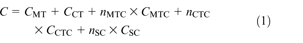
where
GA
The GA generates the FMS solutions according to the following procedure:
Step 1. Get the workpiece manufacturing information such as the features and TADs.
Step 2. Get the GA parameters such as the main population, crossover
Step 3. Generate random solutions for the main population; then, evaluate and save the solutions as the main population.
Step 4. Do the following steps:
Step 4.1. Generate and evaluate new solutions (children) by the crossover (based on the crossover probability). Step 4.2. Apply the mutation on the generated children and assess the results (based on the mutation probability). Step 4.3. Add the results to the main population. Step 4.4. Separate some members of the resulting population such that a new main population as large as the initial main population (Step 2) is created. Step 4.5. End the algorithm if the convergence condition is satisfied; otherwise, go to Step 4.1 and follow the procedure.
The manner by which the initial random population is generated, the way the crossover and mutation are applied, and the parents and the next generation are selected considerably affects the GA. Based on the literature, the method proposed by Su et al. 12 for the generation of the random main population and the tournament selection10–12 is superior to other methods. Crossover and mutation are employed to generate new solutions. In crossover, only the FMS varies and the MRs are assumed unchanged. The preferred crossover technique, namely the ordered crossover, has been proposed by Lee et al. 1 The preferred MR change technique has been proposed by Su et al. 12
Modified particle swarm optimization
The procedure by which PSO determines the FMS is as follows:
Step 1. Get the manufacturing information of the workpiece such as the features and TADs.
Step 2. Get the PSO parameters such as the number of particles, crossover probability, mutation probability, and adjacent swapping parameters.
Step 3. Assign and assess the initial random position and velocity of the particles.
Step 4. Do the following steps:
Step 4.1. Update the particles’ velocity. Step 4.2. Calculate and evaluate the new positions of the particles (new solutions). Step 4.3. Change and assess the position and velocity of the particles by crossover (based on the crossover probability). Step 4.4. Change and assess the particles’ MR by mutation (based on the mutation probability). Step 4.5. Modify the particle’s velocity and position by adjacent swapping (based on the adjacent swapping probability). Step 4.6. End the algorithm provided that the convergence condition is satisfied; otherwise, go to Step 4.1.
As the PSO is designed for continuous environments, it requires “encoding” and “decoding” for discrete environments. Once the position of the particles has changed, the FMS should be specified by decoding. Regarding the particles’ positions, the FMS is specified and the MRs remain fixed. According to the literature, the solutions resulted in this step are not satisfactory and the mutation, crossover, and adjacent swapping are also employed to generate more appropriate solutions.15,16 Recently, Miljković and Petrović 17 have defined velocity and position for the MRs so that they could also be enhanced.
The initial position and velocity of the particles are randomly specified. A value in [0, 1] range is assigned for the particle’s position. The particle’s velocity is represented by a value in [−1, 1] range. The position and velocity in the iteration Itr are then updated as follows
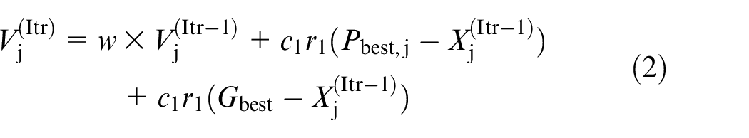
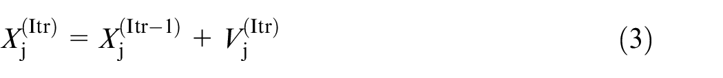
where w represents the velocity weight,
SA
Despite the above algorithms, the SA algorithm starts with a single random solution. The steps of this algorithm are as follows:
Step 1. Get the manufacturing information of the workpiece such as the features and TADs.
Step 2. Get the SA parameters such as the initial temperature and the Markov chain parameters.
Step 3. Generate and evaluate a random solution.
Step 4. Do the following steps:
Step 4.1. Repeat Steps 4.1.1 and 4.1.2 for the Markov chain number.
Step 4.1.1. Generate and assess a new solution in the vicinity of the current solution. Step 4.1.2. Get the new solution based on the Boltzmann probability distribution function. Step 4.2. Decrease the algorithm temperature. Step 4.3. End the program if the convergence condition is satisfied; otherwise, go to Step 4.1.
In this algorithm, new solutions are generated through shifting, MR change, and adjacent swapping. The machining rules may not be followed when a new solution is resulted by shifting and adjacent swapping. Therefore, the results are always modified so that they follow the machining rules. In the literature,1,14 only one solution is generated at constant temperature; in other words, the Markov chain of 1 is assumed. However, it would be more appropriate to generate and evaluate several solutions at a constant temperature. 26
In SA, the new solution is received based on the probability

where
A new procedure for MR determination
The costs of the setup and MR changes can be avoided if the MRs of features are intersected. This article suggests a method for MR intersection and employs common MRs of the features. As mentioned earlier, one reason for the enlarged search space of the optimization algorithms is the existence of numerous MRs for single features. The rationale for MR intersection, therefore, is to reduce the search space by avoiding the generation of non-optimal solutions.
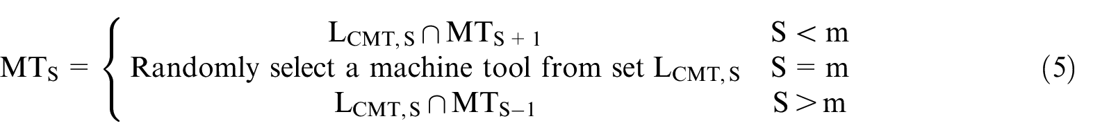
N features are assumed in the workpiece. Hence, the generated sequences consist of N steps and one of the features is machined in each step. The machining steps are denoted by S
The procedure of generating random solutions in optimization algorithms is explained below. First, an FMS is generated. Then, the MRs of each feature are selected among the candidate MRs. In previous methods, the MRs of each feature were randomly selected among the candidate MRs. In this article, a machining step is randomly selected and the MRs of the feature which is machined in this step are randomly chosen among the candidate MRs for that feature. Let the selected machining step be denoted by m. The MRs of the features which are machined after the Step m
Assume an FMS as in Figure 1. The MRs of each feature are to be specified. In this example, only the machine tool of each feature is determined. The cutting tool and TAD also follow the same procedure. As stated previously, a machining step is randomly selected (here, the third step (m = 3)). It is assumed that the machine tool
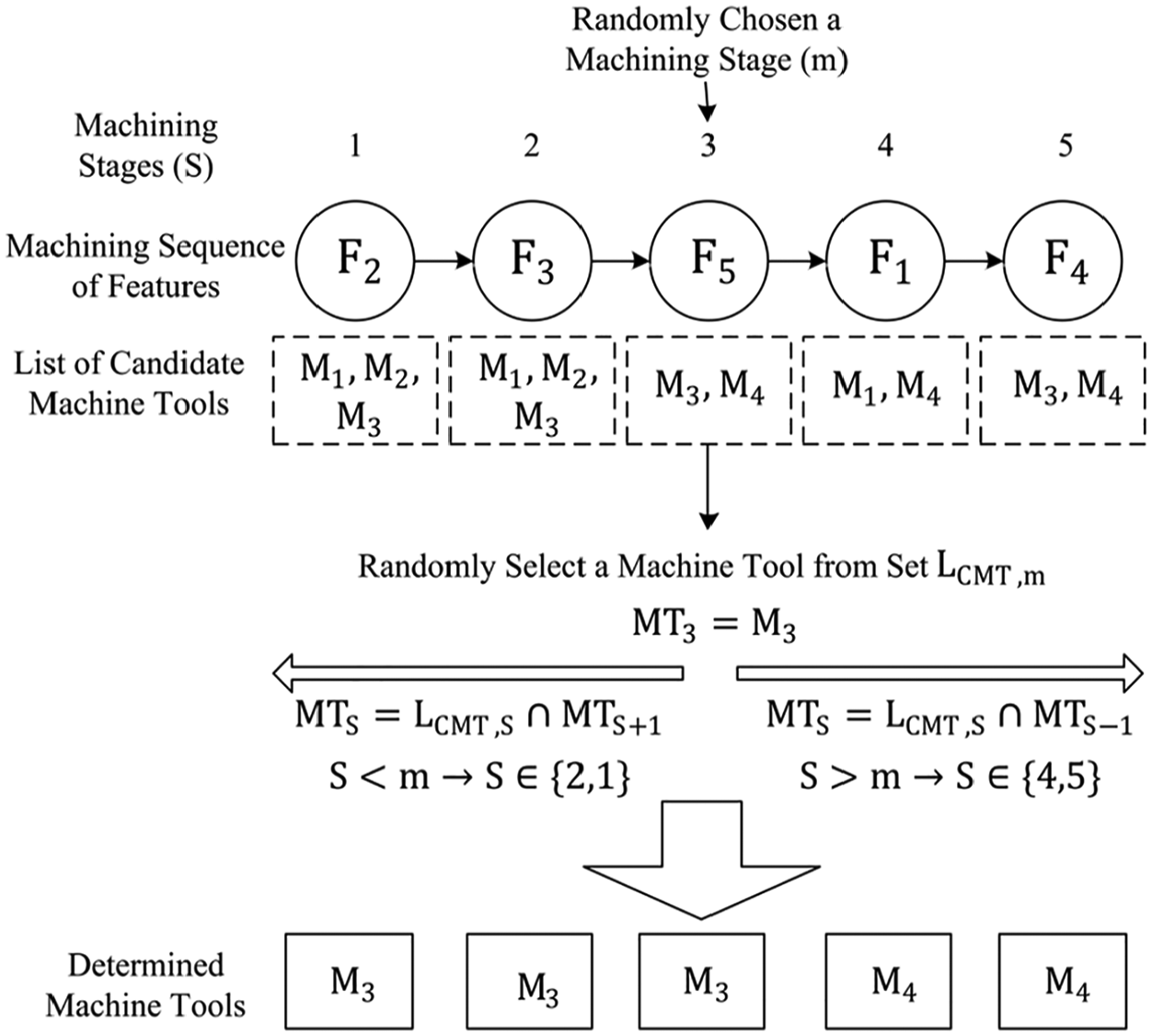
Specifying machine tool for FMS.
In Figure 1, for example, the feature
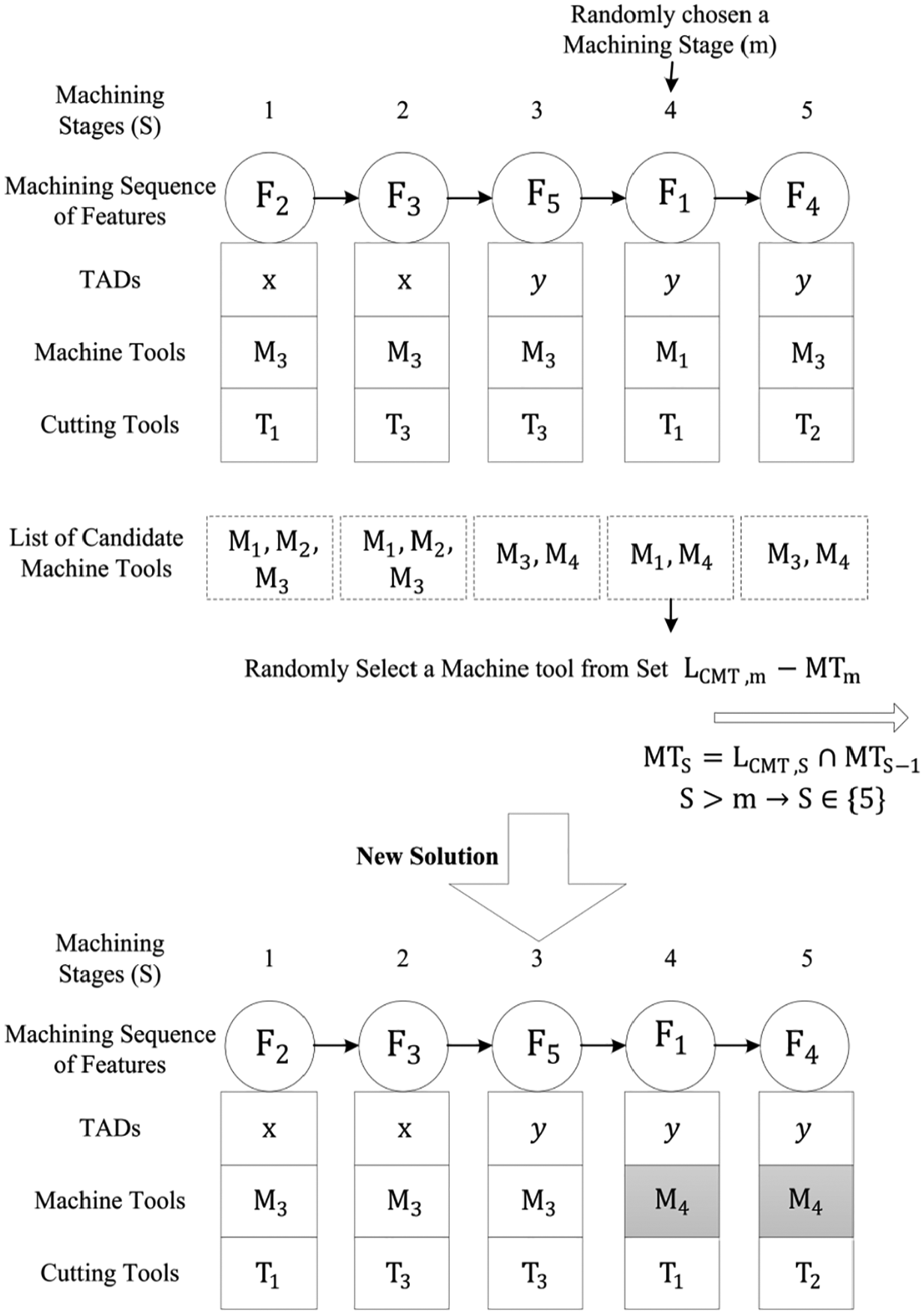
Once the random solutions are generated, the MR type changes through the optimization process so as to create FMSs with different MRs. It should be noted that the MR of each feature is previously determined, but the MR types of some features change in this phase.
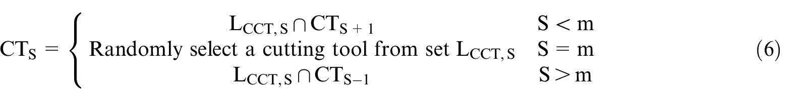
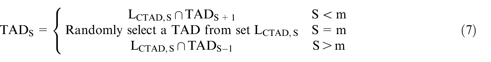
The MR variation method, in this work, differs from those of the literature. The proposed method employs the intersection techniques as follows. First, a specific machining step is randomly chosen (the Step m). Then, an MR of the machine tools, cutting tools, and TAD is selected to be changed later. The variations are only applied to the selected MR. Next, the MR of the Step m is excluded from the candidate MRs. Then, an MR is selected randomly from the remaining MRs. After the Step m

An example of MR change.
An equation similar to equation (8) is used to change the cutting tool and TAD. It should be noted that a null
As previously mentioned, MR variation is applied to only one of the MRs of the TAD, machine tool, and cutting tool; in other words, all MR types do not vary simultaneously. A variation probability is assigned to variation of each MR. This probability specifies the MR which undergoes changes. The variation probability for the machine tool, cutting tool, and TAD is, respectively, designated by
Case study
The algorithms and procedures stated in previous sections are applied in this section. The main characteristics of these algorithms are summarized in Table 1. Considering all necessary parameters, the conventional MR determination methods are replaced by the proposed method and the results are evaluated. The convergence condition is defined as 40,000 function evaluations. The parameters listed in Table 1 are chosen based on trial-and-error.
The characteristics and parameters of optimization algorithms.
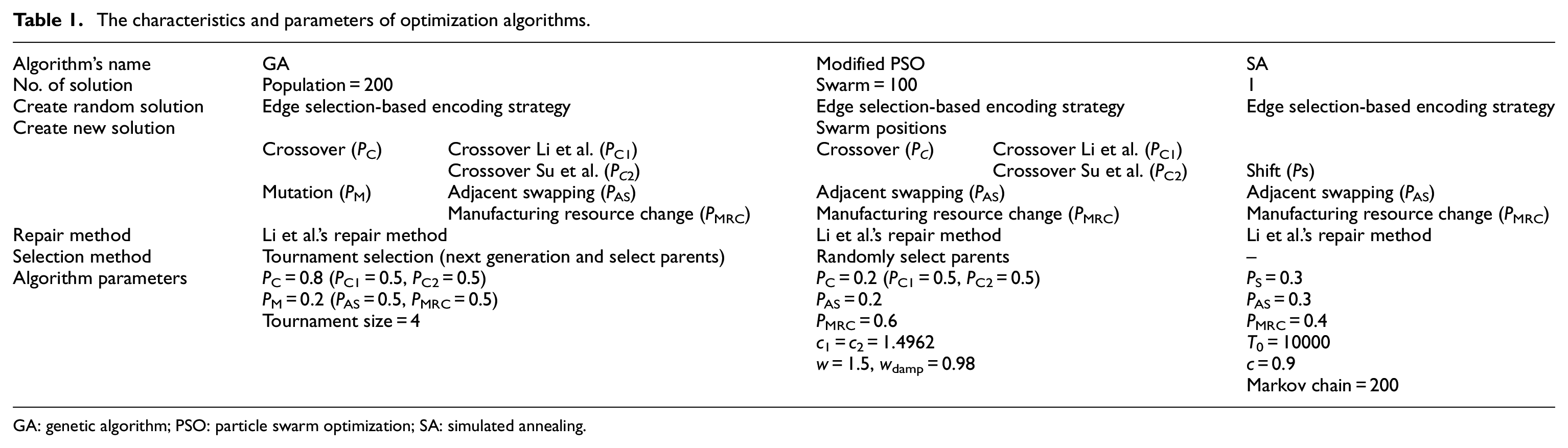
GA: genetic algorithm; PSO: particle swarm optimization; SA: simulated annealing.
The workpiece depicted in Figure 3 is used to evaluate the proposed method. The manufacturing information is summarized in Table 2. In this table, the machine tools are represented by
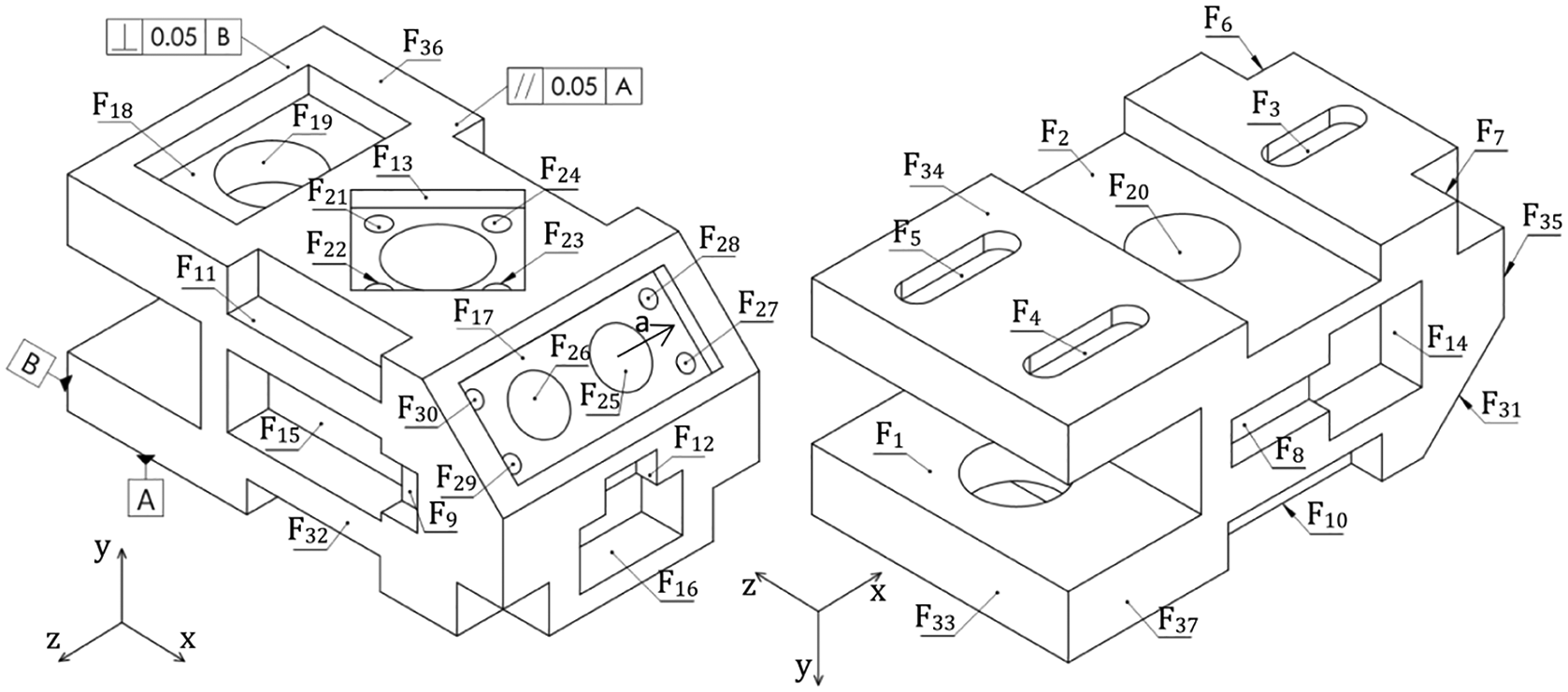
The workpiece.
Manufacturing information of the workpiece.
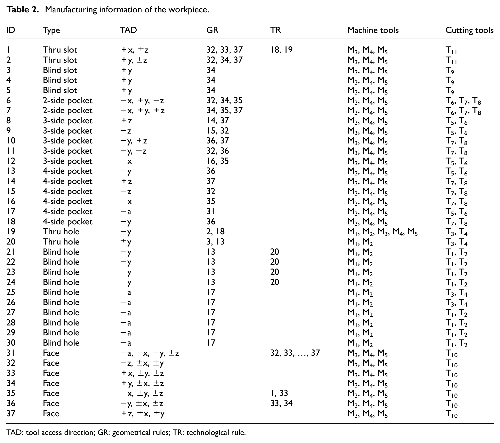
TAD: tool access direction; GR: geometrical rules; TR: technological rule.
In Table 2, the drilling machines are denoted by M1 and M2 and the milling machines are represented by M3, M4, and M5. T1 and T2 are small-sized drilling tools, T3 and T4 are drilling tools, T5 and T6 are small-sized end cutters, T7 and T8 are end cutters, T9 is the slot cutter, T11 is the big-sized slot cutter, and T10 represents the face cutter tool.
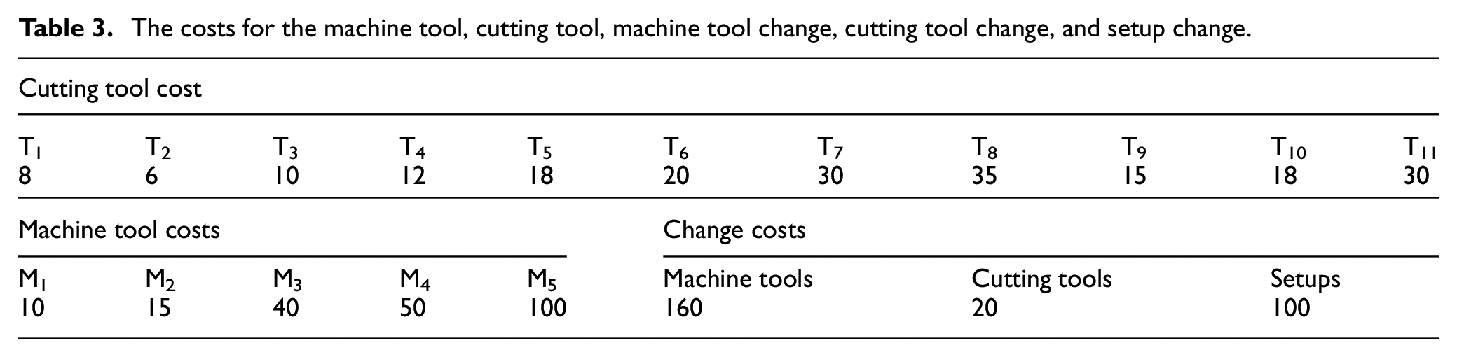
The costs for the machine tool, cutting tool, machine tool change, cutting tool change, and setup change are listed in Table 3.
The costs for the machine tool, cutting tool, machine tool change, cutting tool change, and setup change.
Due to the random nature of the optimization algorithms, each algorithm is run 30 times. The results are listed in Table 4. As previously mentioned, all three MRs do not vary simultaneously, rather one of them changes based on the variation probability. In this case study, the number of machine tools and cutting tools for each feature are close to each other (Table 2). The same variation probability is, therefore, considered for the machine tools and cutting tools. The variation probability of TAD
The results for 30 runs of GA, MPSO, and SA algorithms.
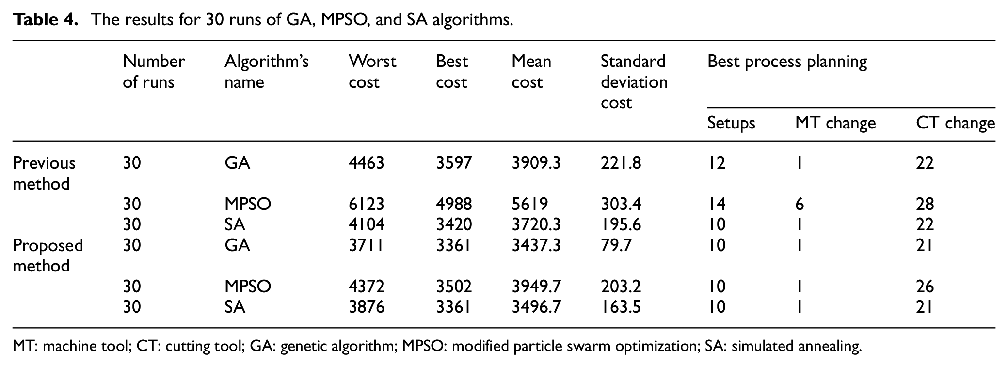
MT: machine tool; CT: cutting tool; GA: genetic algorithm; MPSO: modified particle swarm optimization; SA: simulated annealing.
As it is seen in Table 4, the proposed MR determination method has enhanced the outcome of the optimization algorithms, including the statistical results and the optimal solution. The number of setups, machine tool change, and cutting tool change are similar or close to each other in the obtained FMS in all the three algorithms. It is concluded that the proposed procedure can be implemented in these algorithms. The convergence rate curves of these algorithms are illustrated in Figure 4. The convergence of the optimization algorithms with the conventional and proposed MR determination techniques can be seen in Figure 4(a) and (b), respectively. The convergence curves represent the average results for 30 runs. Although the convergence behavior of both proposed and conventional MR determination methods has some similarities, they considerably differ in two factors. The first factor is the initial cost function value. As it can be seen, the initial cost function value for the conventional methods is close to 9000 (Figure 4(a)). But, the initial cost function value for the proposed method amounts to only 6000. In other words, superior initial solutions are obtained and trivial non-optimal solutions are not generated. The second dissimilarity is the convergence rate which is noticeably better for the proposed algorithm. For enhanced illustration, the convergence curves are shown in terms of the algorithm type in Figure 5. The convergence of the GA with the conventional and proposed MR determination techniques is depicted in Figure 5(a). The enhancement of the convergence rate can be seen in all three algorithms.
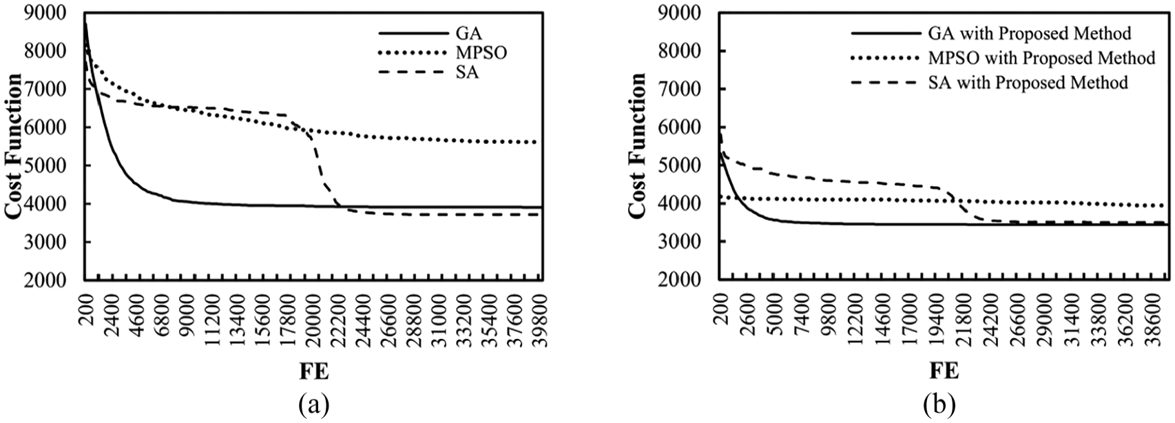
Comparison of convergence curves of optimization algorithms using (a) conventional techniques and (b) the proposed technique for MR determination.
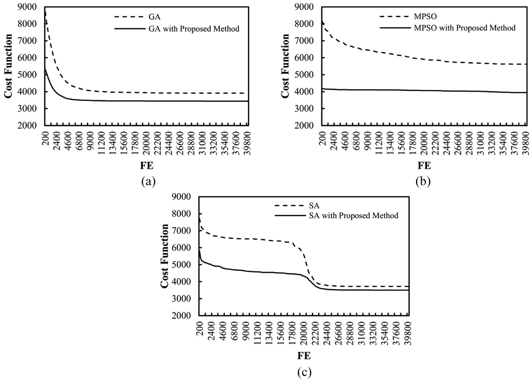
Comparing convergence curves of (a) GA, (b) MPSO, and (c) SA algorithms.
As is seen in Figure 4(a) and Table 4, the best results for MR determination with conventional method belongs to the SA algorithm where the convergence rate is slower than the GA. The SA outperforms the GA in four statistical factors listed in Table 4. If the proposed MR determination technique is employed, the performance of the GA in finding the optimal solution will resemble that of SA, but the GA outperforms the SA in three statistical factors of worst value, average value, and standard deviation of the cost functions. Lower standard deviation in GA shows that closer results are obtained from all 30 runs. Therefore, the best performance from the viewpoint of statistical results and the convergence rate belongs to GA with the proposed MR determination technique.
Although the proposed MR determination technique has enhanced the MPSO results, it still has the worst performance compared to other algorithms. The cost function value of the initial solutions does not considerably differ from that of the final solutions (Figure 5(b)) for the MPSO algorithm; in other words, fewer enhancements are seen in MPSO solutions. Therefore, the MPSO strategy in generating new solutions is weak compared to its counterparts.
Figure 6 depicts the FMS outcome of the GA and SA algorithms. The number of setups is specified based on this FMS. As it can be noticed, these two optimal solutions have slight differences with identical cost function values. These differences can affect the performance of the optimization algorithms. In the MPSO algorithm, for example, the best position of the particles highly affects the new position of all particles. Hence, the variations of the optimal FMS with fixed cost function values can result in continuous variation of the particle movements, so that the algorithm converges to no unique optimal solution.
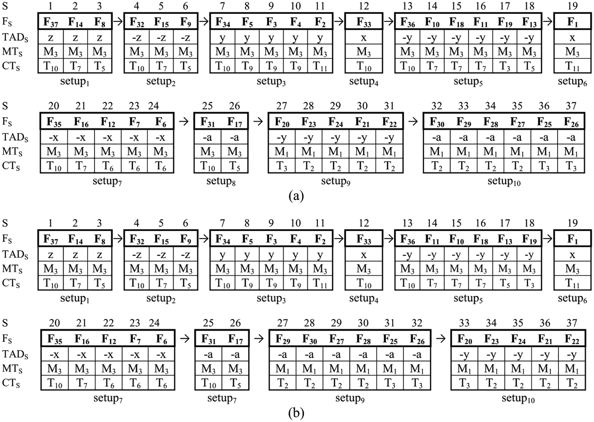
The optimal solutions of (a) GA and (b) SA algorithms.
One difference of the optimal solutions in Figure 6 lies in setup 5 where the features F10, F11, F13, F18, and F19 are placed in different sequences in one setup. This happens due to the lack of GR and TR in these features. In this case, the machining priority is for the feature with the most machining volume. In optimization algorithms, however, this priority either cannot be applied to the features without inter-related rules or it requires auxiliary algorithms.
It should be noted that the number of setups is not optimized, but it is specified based on the FMS. Although taking the setup change costs into account can reduce the number of setups, it cannot guarantee setup minimization. Consider an example in which one setup can be separated into two different setups with less machining costs. This may seem favorable, but it can also increase the machining errors and necessitate the tolerance analysis so that the workpiece tolerances are followed. Due to similar reasons and existence of several optimal solutions (Figure 6), an appropriate cost function has to be defined for setup planning.
Conclusion
Determination of setup and machining sequence is a major part of CAPP. Various methods, including the optimization algorithms, have already been proposed by the researchers for this purpose. In this work, three optimization procedures, including the GA, SA, and PSO algorithms, have been studied. These algorithms suffer from large search space. One reason for this large space is various MRs for a single machining feature. Hence, a method based on MR intersection has been proposed for reducing the search space. This method avoids trivial non-optimal solutions in which unnecessary cutting tool, machining tool, and setup change costs are involved. The proposed method has been tested on the above-mentioned algorithms. The results prove the enhanced performance of these algorithms. The MR determination method has enhanced the outcome of the optimization algorithms, including the statistical results and the optimal solution. It is concluded that the proposed procedure can be implemented in these algorithms. The best and the worst performances were observed in the GA and PSO, respectively.
Footnotes
Appendix 1
Declaration of conflicting interest
The author(s) declared no potential conflicts of interest with respect to the research, authorship, and/or publication of this article.
Funding
The author(s) received no financial support for the research, authorship, and/or publication of this article.