Sage Journals: Discover world-class research

Abstract

The integration of process planning and scheduling is a very important problem because it proposes a new idea for improving the performance of a manufacturing system. At present, most existing studies on this problem are static, which assumes that all the jobs to be processed are available in the beginning. However, the practical processing situation is dynamic, such as new job arrivals. Since dynamic production situations are different with static cases, it is important to study the characteristics of actual production situations. In this article, the characteristics of dynamic integrated process planning and scheduling problem with job arrivals are studied. A novel mixed integer linear programming model is established to accommodate new job arrivals, and three criteria (makespan, stability, and tardiness) are considered. New periodic and event-driven rescheduling strategies are presented. In the proposed strategy, newly added jobs together with uncompleted jobs will be rescheduled by non-dominated sorting genetic algorithm-II to obtain the optimal Pareto front when the rescheduling procedure is triggered. The entropy-based weight assigning method together with the Technique for Order of Preference by Similarity to Ideal Solution method is adopted to determine an appropriate schedule among the resultant non-dominated solutions. A set of well-known benchmark instances is employed to investigate the characteristics of the dynamic integrated process planning and scheduling problem with random job arrivals. Experimental results show that the length of a scheduling interval, the number of newly added jobs, and the shop utilization have an important influence on the efficiency of a manufacturing system.

Keywords

Dynamic scheduling integrated process planning and scheduling TOPSIS NSGA-II

Introduction

Process planning and scheduling are two important functions in a manufacturing system.^1,2 The former focuses on determining appropriate machine tools, resources, and processing schemes,^3–5 while the latter allocates operations to each machine with certain criteria. Usually, based on the divide and rule principle,⁶ the two functions are performed in a successive and independent sequence:^7–9 scheduling will be carried out after the process planning. This paradigm ignores the inherent relationship between the two functions. Drawbacks caused by splitting the two functions, for example, low facility utilization, high scheduling conflicts, and more human intervention, have been well identified and discussed.^7,10–12 Realizing the existing drawbacks, researchers have developed lot of approaches to address the integrated process planning and scheduling (IPPS) problem. Two kinds of solution methodologies are covered in existing papers: mathematical programming approaches and approximation approaches, for example, meta-heuristic algorithms and artificial intelligence methods. Özgüven et al.¹³ proposed mixed integer linear programming (MILP) models to deal with the problem; however, their models are suitable for small-scale instances only. Tan and Khoshnevis¹⁴ transformed a non-linear model into an MILP model for the IPPS problem. Nevertheless, due to the excessive CPU time, applications of mathematical programming are limited. Meta-heuristic-based algorithms have garnered tremendous attentions and have been widely adopted due to their impressive features, such as short computational time. Kim et al.¹⁵ are among the pioneers who studied the IPPS problem; they reported a typical set of benchmark instances (Kim’s benchmark) which are further solved by their developed symbiotic evolutionary algorithm (SEA). Later, Shao et al.¹⁶ proposed a genetic algorithm (GA)-based approach for solving small-scale IPPS instances. Concerning Kim’s benchmark, Lian et al.⁷ suggested a novel algorithm, the imperialist competitive algorithm (ICA), to settle this problem although the improvements of Kim’s benchmark are limited. Li et al.¹⁷ further developed another effective GA-based hybrid algorithm for the IPPS problem; in their algorithm, a tabu search with an effective neighborhood structure is employed.¹⁸ Later, they again developed a novel active learning genetic algorithm (ALGA) by introducing an active learning effect into GA.¹⁹ In recent years, Lihong and Shengping²⁰ suggested an improved genetic algorithm (IGA) for this problem, and new genetic representations with genetic operators were developed. Substantial progress has been observed in Zhang and Wong’s work;²¹ an object-coding GA for the IPPS problem was reported in their work. Other than the approaches mentioned above, other approaches can also be observed, including the grammatical optimization approach,²² the simulated annealing-based optimization approach,²³ the modified particle swarm optimization (PSO) algorithm,²⁴ and agent-based methods.²⁵

A great deal of IPPS problems have been studied. However, a manufacturing system in the real world is often subject to many sources of uncertainty. One main source of uncertainty lies in random job arrivals. Thus, a predefined schedule will fail unless a timely new schedule is prepared. In a dynamic situation, a new feasible schedule, which takes in account the new jobs and unfinished jobs, will be generated when a new job arrival occurs. The process of generating a new feasible schedule in response to the unexpected disturbances is recognized as the rescheduling process. There are two kinds of rescheduling strategies in general: periodic and event-driven rescheduling strategies. In periodic rescheduling, a new schedule is generated after a certain scheduling interval. In event-driven rescheduling strategy, the rescheduling procedure is triggered whenever new job arrivals occur. As claimed in relative papers,^26,27 the new schedule may suffer from a greater deviation to the original schedule and the initial schedule will not be preserved any more. In such a case, pre-allocated resources for each machine, such as raw materials, will be altered. What’s more, the unfinished jobs may be put off, and hence, the tardiness should be considered as another criterion in dynamic scheduling except the makespan and the stability criteria. In this article, the multi-objective issue is addressed in a Pareto manner.

Existing papers pay more attention to the rescheduling strategies for job shop scheduling problems (JSPs)^27–29 and flexible job shop scheduling problems (FJSPs).³⁰ The only two studies about the rescheduling of IPPS problems are reported by Lv and Qiao³¹ and Wong et al.,²⁶ respectively. Lv and Qiao considered new job arrivals, machine breakdowns, and order cancelations simultaneously, and their algorithm achieved satisfactory makespan values. Wong et al. presented a hybrid multi-agent system (MAS) to address the dynamic IPPS problem with machine breakdowns and new part arrivals. However, it is worth mentioning that the study on the impacts of rescheduling has scarcely been considered. It cannot be denied that different parameters in rescheduling, for example, the length of a scheduling interval, have important impacts on the performance of schedulings. However, one cannot tell which disturbance is the dominant one and how it affects the performance of a manufacturing system. The primary goal of this research is to give a minute study on the factors (e.g. interval length) that affect the performance of a manufacturing system with new job arrivals over time. We consider both periodic and event-driven rescheduling strategies in this article, and new job arrivals are deemed as disturbances. An MILP model for the dynamic IPPS problem is established. Then, the non-dominated sorting genetic algorithm-II (NSGA-II)-based solution methodology for rescheduling is presented. At each rescheduling point, a new schedule is generated for the coming scheduling interval. To strike a compromise between the three criteria (makespan, tardiness, and stability), the entropy-based weight assignment method and the Technique for Order of Preference by Similarity to Ideal Solution (TOPSIS) decision-making strategy are employed to determine the most appropriate schedule for the coming scheduling interval. Finally, the Kim’s instances are adopted as the test-bed instances in the experimental study.¹⁵

The remaining sections are organized as follows: Section “Problem description” gives the preliminaries of the dynamic IPPS problem. A novel MILP model will be proposed in section “Mathematical modeling.” In section “NSGA-II-based solution methodology,” we describe the details of the proposed NSGA-II-based methodology. Experimental results with discussions will be presented in section “Experiments with discussions.” Some concluding remarks are given in section “Conclusion.”

Problem description

In this research, a mathematical model is established to express the inherent nature and important characteristics of the dynamic IPPS problem. The proposed model is extended from the model of the static IPPS problem.¹⁹ The proposed model generates a schedule for the next rescheduling interval, and the subscript p is introduced to distinguish between the unfinished jobs and new jobs. This classifies all the jobs into two kinds: the unfinished jobs and the new jobs, and hence it is easy to schedule the two kinds of jobs in the model. Then, an NSGA-II-based methodology is proposed. In this method, the whole time interval is divided into several intervals by rescheduling points. A rescheduling point is the time when a new schedule is constructed. At each rescheduling point, the schedules are optimized by NSGA-II and a new schedule is determined by the TOPSIS method as the schedule for the following interval. When a rescheduling point is encountered or a new job arrival occurs, this process is repeated until all the jobs are finished. Apparently, the proposed methodology is close to the real-world situations.

The IPPS problem can be defined as follows:²⁴ Given a set of n parts (jobs) to be processed on m machines with operations including alternative manufacturing resources, select the suitable manufacturing resources and sequence the operations so as to determine a schedule in which the precedence constraints among operations can be satisfied and the corresponding objectives can be achieved. In dynamic situations, jobs arrive continuously over time.

This problem can be expressed by a network graph as illustrated in Figure 1(a)). In the network graph, the starting node and the ending node are two dummy nodes which represent fictitious operations with processing time zero and do not require any machines. Other nodes are operation nodes. In an operation node, the operation number with its alternative machines and corresponding processing times are specified. An arrow between two nodes specifies a precedence relationship of the two operations: if operation node A points to node B, then operation B should follow operation A directly or indirectly. Moreover, if a bifurcation is marked with “OR,” this means that only one OR link path of the two should be traversed. In other cases, the two link paths of a bifurcation both should be traversed (see Figure 1(a)).

Figure 1.

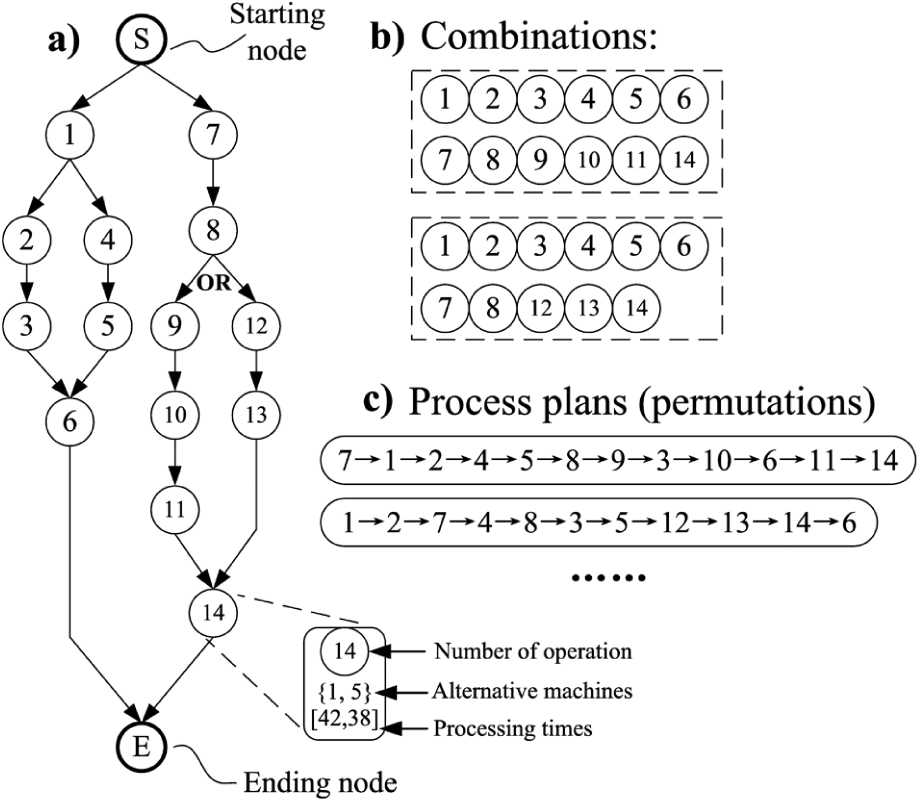
A network graph.

For a given network graph, operation combinations can be first determined by visiting different OR link paths. In Figure 1(b), there are two combinations. After that, a process plan can be generated by adopting one of the feasible operation permutations generated from a combination. Two possible process plans, generated from the two combinations, are given in Figure 1(c)).

In a real job shop, as illustrated in Figure 2, jobs arrive continuously over time at either specified or random arrival dates. In each rescheduling point t_i, the operations that need rescheduling consist of two parts: operations of new jobs and unfinished jobs (unprocessed operations) in the previous interval. Suppose the current time is t_i, the interval between t_i₋₁ and t_i is a rescheduling interval, and new job arrivals occur at the rescheduling point t_i. ΔT₁ and ΔT₂ are the lengths of two intervals. In periodic rescheduling, the two values are equal; in event-driven rescheduling, the length of each interval follows an exponential distribution. At current time t_i, a new schedule should be determined using NSGA-II and the TOPSIS method for the coming interval between t_i and t_i+₁.

Figure 2.

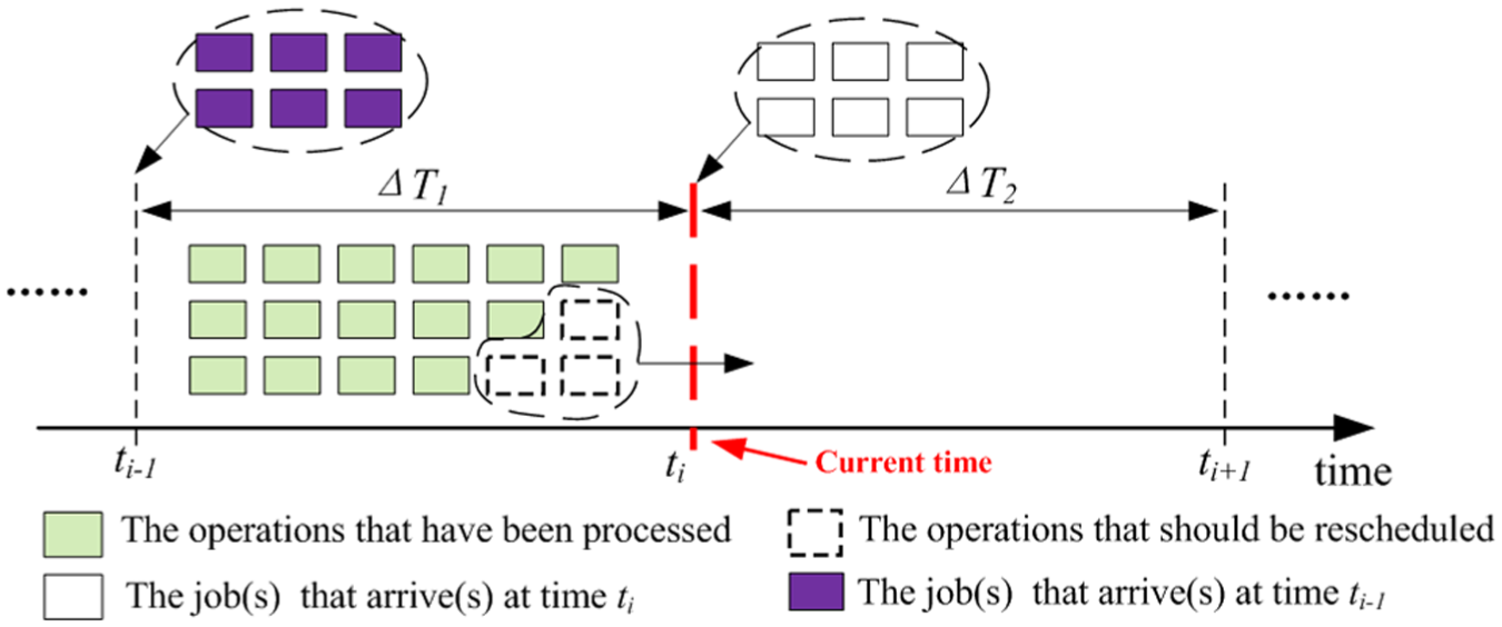
A rescheduling strategy.

Mathematical modeling

The MILP model of the dynamic IPPS problem is extended from the models of the static and mono-objective IPPS problem,^19,32 and it is established based on the following assumptions:

Jobs and machine tools are independent, and all the machines are available at time zero.

Each machine can handle at most one job at a time, and different operations of a job cannot be processed at the same time.

Job pre-emption is not allowed.

Within a rescheduling interval, a job will be immediately transferred to another machine for the next operation after the current operation is finished with the time for transferring neglected. Between different intervals, the starting time of an unfinished job depends on the new schedule.

Setup time of an operation can be included in the processing time.

Notations, sets, parameters, and variables used in this model are furnished in Appendix 1.

In this model, the letter “p” in subscripts refers to the situation where unfinished jobs in last interval are involved:

Objectives

Min C_{max}, S, T

(1)

s.t.

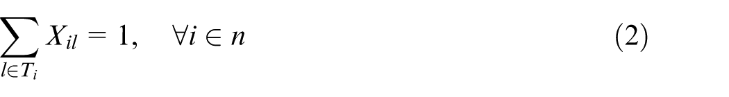
For new jobs, each job should select exactly one process plan as stated in constraint set (2). For the unfinished jobs in last interval, corresponding process plans have already been determined

\sum_{l \in T_{i}} X_{il} = 1, \forall i \in n

(2)

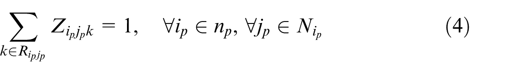
The operations belonging to the unselected process plans are eliminated; otherwise, each selected operation is assigned to exactly one machine

\sum_{k \in R_{ijl}} Z_{ijkl} = X_{il}, \forall i \in n, \forall l \in T_{i}, \forall j \in N O_{il}

(3)

For operations of the unfinished jobs, each of them should be processed by exactly one machine

\sum_{k \in R_{i_{p} j_{p}}} Z_{i_{p} j_{p} k} = 1, \forall i_{p} \in n_{p}, \forall j_{p} \in N_{i_{p}}

(4)

The starting time of each new job should be no earlier than the rescheduling point

C_{i, 0} ⩾ ST, \forall i \in n

(5)

Each unfinished job should start at a proper time as shown in constraint set (6)

C_{i_{p} j_{p}} ⩾ max {J T_{i_{p}}, ST}, \forall i_{p} \in n_{p}, \forall j_{p} \in N_{i_{p}}

(6)

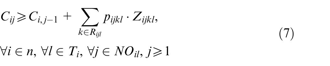
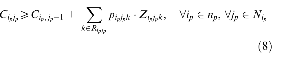
Following two constraint sets are introduced to schedule two sequential operations of the same job. Constraint set (7) schedules two sequential operations of a new job; constraint set (8) schedules two sequential operations of an unfinished job in the previous interval. After this, a correct precedence relationship between two operations of the same job is guaranteed because the completion time of the latter operation should be equal or greater than the completion time of the former plus the processing time

\begin{array}{l} C_{i j} ⩾ C_{i, j - 1} + \sum_{k \in R_{i j l}} p_{i j k l} \cdot Z_{i j k l}, \\ \forall i \in n, \forall l \in T_{i}, \forall j \in N O_{i l}, j ⩾ 1 \end{array}

(7)

C_{i_{p} j_{p}} ⩾ C_{i_{p}, j_{p} - 1} + \sum_{k \in R_{i_{p} j_{p}}} p_{i_{p} j_{p} k} \cdot Z_{i_{p} j_{p} k}, \forall i_{p} \in n_{p}, \forall j_{p} \in N_{i_{p}}

(8)

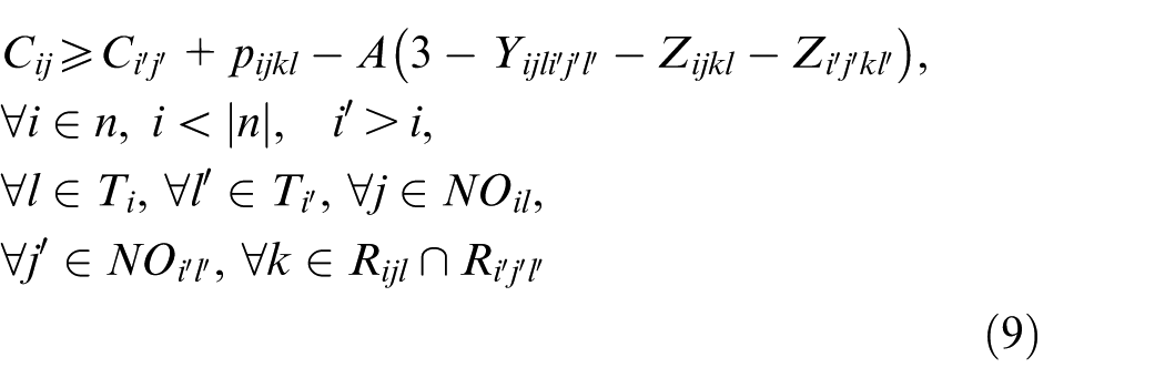
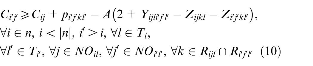
Constraint sets (9) and (10) state that a precedence relationship between two operations, which belong to two different new jobs and to be processed on the same machine, should be satisfied

\begin{matrix} C_{ij} ⩾ C_{i' j'} + p_{ijkl} - A (3 - Y_{ijli' j' l'} - Z_{ijkl} - Z_{i' j' kl'}), \\ \forall i \in n, i < | n |, i' > i, \\ \forall l \in T_{i}, \forall l' \in T_{i'}, \forall j \in N O_{il}, \\ \forall j' \in N O_{i' l'}, \forall k \in R_{ijl} \cap R_{i' j' l'} \end{matrix}

(9)

\begin{matrix} C_{i' j'} ⩾ C_{ij} + p_{i' j' kl'} - A (2 + Y_{ijli' j' l'} - Z_{ijkl} - Z_{i' j' kl'}), \\ \forall i \in n, i < | n |, i' > i, \forall l \in T_{i}, \\ \forall l' \in T_{i'}, \forall j \in N O_{il}, \forall j' \in N O_{i' l'}, \forall k \in R_{ijl} \cap R_{i' j' l'} \end{matrix}

(10)

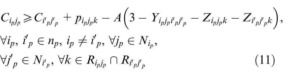
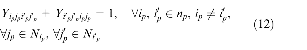
Similarly, constraint sets (11) and (12) reschedule two unfinished jobs on the same machine such that a precedence relationship between two unfinished jobs on the machine is established

\begin{matrix} C_{i_{p} j_{p}} ⩾ C_{{i'}_{p} {j'}_{p}} + p_{i_{p} j_{p} k} - A (3 - Y_{i_{p} j_{p} {i'}_{p} {j'}_{p}} - Z_{i_{p} j_{p} k} - Z_{{i'}_{p} {j'}_{p} k}), \\ \forall i_{p}, {i'}_{p} \in n_{p}, i_{p} \neq {i'}_{p}, \forall j_{p} \in N_{i_{p}}, \\ \forall {j'}_{p} \in N_{{i'}_{p}}, \forall k \in R_{i_{p} j_{p}} \cap R_{{i'}_{p} {j'}_{p}} \end{matrix}

(11)

\begin{array}{l} Y_{i_{p} j_{p} {i^{'}}_{p} {j^{'}}_{p}} + Y_{{i^{'}}_{p} {j^{'}}_{p} i_{p} j_{p}} = 1, \forall i_{p}, {i^{'}}_{p} \in n_{p}, i_{p} \neq {i^{'}}_{p}, \\ \forall j_{p} \in N_{i_{p}}, \forall {j^{'}}_{p} \in N_{{i^{'}}_{p}} \end{array}

(12)

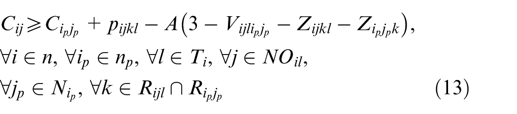
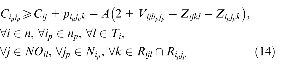
Since there are two kinds of jobs—the new jobs and the unfinished jobs—a precedence relationship between a new job and an unfinished job on the same machine is specified by constraint sets (13) and (14)

\begin{matrix} C_{ij} ⩾ C_{i_{p} j_{p}} + p_{ijkl} - A (3 - V_{ijl i_{p} j_{p}} - Z_{ijkl} - Z_{i_{p} j_{p} k}), \\ \forall i \in n, \forall i_{p} \in n_{p}, \forall l \in T_{i}, \forall j \in N O_{il}, \\ \forall j_{p} \in N_{i_{p}}, \forall k \in R_{ijl} \cap R_{i_{p} j_{p}} \end{matrix}

(13)

\begin{matrix} C_{i_{p} j_{p}} ⩾ C_{ij} + p_{i_{p} j_{p} k} - A (2 + V_{ijl i_{p} j_{p}} - Z_{ijkl} - Z_{i_{p} j_{p} k}), \\ \forall i \in n, \forall i_{p} \in n_{p}, \forall l \in T_{i}, \\ \forall j \in N O_{il}, \forall j_{p} \in N_{i_{p}}, \forall k \in R_{ijl} \cap R_{i_{p} j_{p}} \end{matrix}

(14)

Constraint sets (15), (16), and (17) determine the values of three objectives. Constraint set (15) determines the makespan, and constraint set (16) determines the total tardiness of all the job

C_{max} ⩾ C_{ij}, \forall i \in n, \forall i_{p} \in n_{p}, \forall j \in N O_{il}, \forall j_{p} \in N_{i_{p}}

(15)

\begin{array}{l} T = \sum_{i \in n} \sum_{j \in N O_{i l}} \max {0, \max {C_{i j}} - D D_{i}} \\ + \sum_{i_{p} \in n_{p}} \sum_{j_{p} \in N_{i_{p}}} \max {0, \max {C_{i_{p} j_{p}}} - D D_{i_{p}}} \\ \forall i \in n, \forall i_{p} \in n_{p}, if C_{i, | N O_{i j} |} ⩽ S T^{'}, and C_{i_{p}, | N_{i_{p}} |} ⩽ S T^{'} \end{array}

(16)

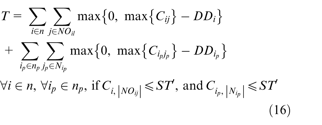
The last objective is about the stability. Two stability indicators related to the part’s and machine’s deviation costs are measured in constraint set (17). Once an operation is pre-scheduled on a machine, corresponding manufacturing resources, such as raw materials and human workers, are expected to be ready right before its starting time. Any changes of its starting time will alter the resource allocation, and hence, the resources are either expedited or delayed to cope with the new schedule.²⁶ In constraint set (17), $| C_{i_{p} j_{p}} - \sum_{k \in R_{i_{p} j_{p}}} p_{i_{p} j_{p} k} Z_{i_{p} j_{p} k} - s t_{i_{p} j_{p}} |$ stands for the deviation of the starting time between the original schedule and the new schedule. Similarly, the second term in constraint set (17) expresses machines’ deviation costs

\begin{array}{l} S = \sum_{i_{p} \in n_{p}} \sum_{j_{p} \in N_{i_{p}}} (d_{i_{p} j_{p}} | C_{i_{p} j_{p}} - \sum_{k \in R_{i_{p} j_{p}}} p_{i_{p} j_{p} k} Z_{i_{p} j_{p} k} - s t_{i_{p} j_{p}} |) \\ + q_{k} (\sum_{k \in M} | \sum_{i_{p} \in n_{p}} \sum_{j_{p} \in N_{i_{p}}} Z_{i_{p} j_{p} k} - Q_{k} |) \end{array}

(17)

NSGA-II-based solution methodology

Since the dynamic IPPS problem is an extension of the FJSP, it is certainly a strong NP-hard problem. On the other hand, the MILP formula for this problem described above is a multi-objective problem. In this study, the well-known NSGA-II³³ is introduced to cope with the multi-objective dynamic IPPS problem. NSGA-II is deemed as the most powerful meta-heuristic algorithm to address multi-objective problems. The details of the procedure will be described later.

Encoding and decoding

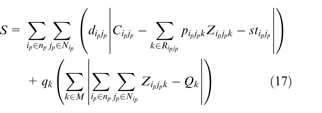
The chromosome structure is illustrated in Figure 3. A chromosome consists of a scheduling string, some process plan strings, and corresponding operation strings. The scheduling string shown in Figure 3 adopts an operation-based coding scheme.³⁴ This coding scheme brings convenience to the decoding process. For a newly added job, the job number in this string appears $| N O_{il} |$ times. For an unfinished job in last interval, its job number (job ID) will appear $| N_{i_{p}} |$ times ( $N O_{il}$ and $N_{i}$ are the sets used in the mathematical model). Moreover, the length of the scheduling string in Figure 3 equals the sum of the maximum possible number of operations of each newly added job plus the number of operations of each unfinished job $(\sum | N O_{il} |_{max} + \sum | N_{i_{p}} |)$ . For a new job i, if the actual number of the operations is less than the maximum possible one $(| N O_{il} | < | N O_{il} |_{max})$ , $(\sum (| N O_{il} |_{max} - | N O_{il} |))$ positions in the scheduling string in Figure 3 should be filled with 0s to avoid any infeasibility. As illustrated in Figure 3, there is an example with three jobs to be scheduled in the forthcoming interval. Suppose that each job has at most three operations and the second job is an unfinished job with two operations (one operation has been processed in last interval); there are nine operations at most, while the actual numbers of operations for the three jobs are three, two, and three. Therefore, the total number of operations in this instance is eight $(\sum | N O_{il} | = 3 + 2 + 3)$ . Since the maximum length of the scheduling string in Figure 3 is nine, in this case, a “0” should be filled in the string.

Figure 3.

The coding scheme.

Other two kinds of strings are about process planning. There are a total of $| n | + | n_{p} |$ operation strings and $| n | + | n_{p} |$ process plan strings. An operation string illustrated in Figure 3 contains the detailed information of operations in a job, and it also specifies the precedence relationships among operations belonging to the same job. There are $| N O_{il} |$ operations in the operation string of a new job, while the number of operations in the operation string of an unfinished job is $| N_{i_{p}} |$ . In each position, the operation number (operation ID) and the corresponding machine for the operation are specified. The number in a process plan string specifies which process plan combination is selected for a job. Once an operation combination (Figure 1(b)) is determined for a job, a feasible permutation of operations in the operation string can be easily generated by using the binary tree method.³⁵

The active scheduling procedure is adopted to transform the chromosome into a feasible schedule scheme. A number i (i≠0) in the scheduling string in Figure 3 is taken each time; if i appears exactly l times in the scheduling string, the operation in the lth position of the operation string of job i is selected. For instance, the number in the second position of the scheduling in Figure 3 is 1, and it appears for the first time. This means it is the first operation of job 1 with operation ID 3 according to the first operation string in Figure 3, and it will be processed by machine 2. The whole decoding procedure is provided as follows:

Step 1. Determine the operation to be scheduled, for example, $O_{ij}$ , using the method discussed above.

Step 2. Assign this operation on the predefined machine $m_{k}$ with processing time $t_{ijk}$ .

Step 2.1. Check whether there is a time slot on machine $m_{k}$ . A time slot is a tiny spare time interval between two adjacent operations that has been assigned on the same machine. Sometimes, there may be no time slot if two operations are close to each other. The stating time and the completion time of a time slot are $t_{s}$ and $t_{e}$ , respectively.

Step 2.2. If there is a time slot and $max {c_{i, j - 1}, t_{s}} + t_{ijk} ⩽ t_{e}$ (suppose $c_{i, j - 1}$ is the completion time of the job predecessor of $O_{ij}$ ), insert the operation in this time slot and go to Step 1 for the next operation. Otherwise, check the next slot on the machine till all the time slots have been checked.

Step 2.3. If there is no available time slot, append $O_{ij}$ at the end of the machine with the starting time $max {c_{i, j - 1}, t_{k}}$ , where $t_{k}$ is the machine available time.

Step 3. Go to Step 1 for the next operation till all the operations are scheduled.

Genetic operators

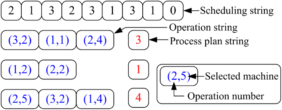
Figure 4 illustrates the crossover procedure. Randomly exchange the operation strings together with corresponding process plan strings of some randomly selected jobs in two individuals; other operation strings and process plan strings in both individuals are kept still. Then, two empty scheduling strings O1 and O2 are initialized. The job IDs in the scheduling string of parent 1 (P1), which reflect the unselected jobs, are passed on to the same positions as in the offspring 1 (O1). These job IDs are removed from parent 2 (P2), and the remaining elements are copied into the undetermined positions in O1 in the same order as they appear in P2. A repairing procedure is adopted to resolve the illegitimacy; it deletes redundant symbols or adds necessary symbols after checking the actual number of operations of each selected job. Figure 4(a)) gives an example. Last two jobs in two different chromosomes are selected, and a “0” is filled in a position in offspring 2 (O2) to avoid infeasibility.

Figure 4.

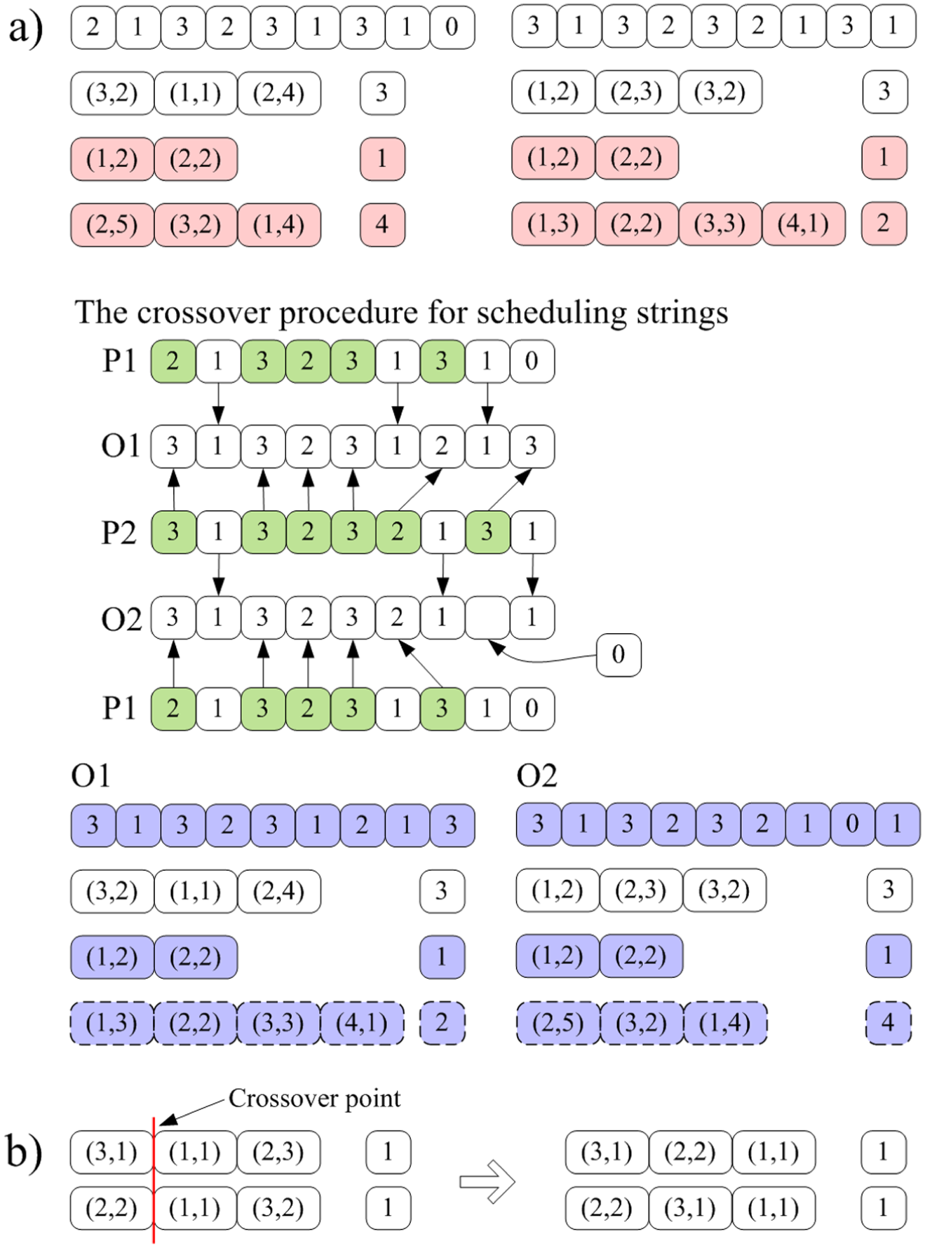
Crossover operators: a) the first crossover operator and b) the second crossover operator.

In the IPPS problem, the same operation combination of a job may have different operation permutations. The proposed coding scheme allows the NSGA-II to take this advantage by performing the second crossover operator as shown in Figure 4(b). An order crossover (OX)-based one-point crossover method is adopted. If two operation strings of a job in two individuals adopt the same combination, this crossover procedure is performed. According to Figure 4(b)), the two operation strings have the same operations because they both adopt the first combination; after that, two new feasible operation stings are generated with new feasible permutations.

For the selection operator, a simple tournament selection is adopted. The mutation procedure is performed by changing a machine for an operation and swapping two numbers in two randomly selected positions in the scheduling string.

Decision method

After the NSGA-II procedure, a Pareto front which contains several non-dominated solutions will be generated. However, only one schedule will be selected for the forthcoming scheduling interval. The TOPSIS method,³⁶ based on the concept that the chosen alternative should have the shortest distance from the ideal solution and farthest from the negative-ideal solution, is adopted. A set of weights for all the objectives in TOPSIS is generated by the entropy-based weight assigning method.³⁶

Objective function

In this article, we consider three objectives: makespan, tardiness, and stability. Makespan is defined as the total time required to process all the jobs. It is calculated by simply taking the difference between the starting time (zero, in this article) and the completion time of the last job. Tardiness is defined as the sum of the difference between the completion time and due date for each job in the case where the job is finished after the due date. For stability, two dimensions of stability are modeled as formulated in equation (17). The first measure is about the total deviations of the starting times between the new schedule and the old schedule for all the unfinished jobs. The second measure associates penalties induced by machines’ deviation costs; it is reflected in the changes of the numbers of unfinished operations on machines as expressed by the second term of equation (17).

Key parameters

In event-driven rescheduling, jobs will arrive at random times over the whole scheduling horizon. A widely accepted fact is that a Poisson distribution provides a good approximation for dynamic job arrivals in a job shop.³⁷ The arrival rate, λ, is assumed to be equal to the ratio of the capability of the shop to the average amount of work required

λ = \frac{M \cdot η}{\bar{n} \cdot \bar{p}}

(18)

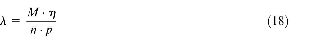
where M is the number of machines, η is the shop utilization (machine load capability), $\bar{n}$ is the average number of operations, and $\bar{p}$ is the average processing time. A variety of arrival patterns can be obtained by adjusting the parameter $η$ . Thus, the degree of congestion in the shop is under control. Furthermore, the length of an interval in a dynamic situation (the time between two rescheduling point) follows an exponentially distribution with 1/λ as its expectation value.

The total work content (TWK) rule is adopted to generate due dates for each job; it equals the sum of the job arrival time and total job processing times

D D_{i} = a_{i} + K \sum_{j} p_{i, j}, \forall i = 1, 2, \dots

(19)

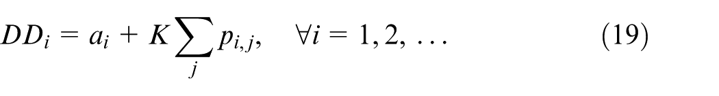
where a_i is the arrival time of job i, K is the tightness factor (in this article, k = 1 for simplicity), and $p_{i, j}$ is the processing time of an operation of job i.

The main framework

Figure 5 illustrates the working flow of the algorithm. At each rescheduling point, unfinished operations are combined with the newly added jobs and a new schedule is established.

Figure 5.

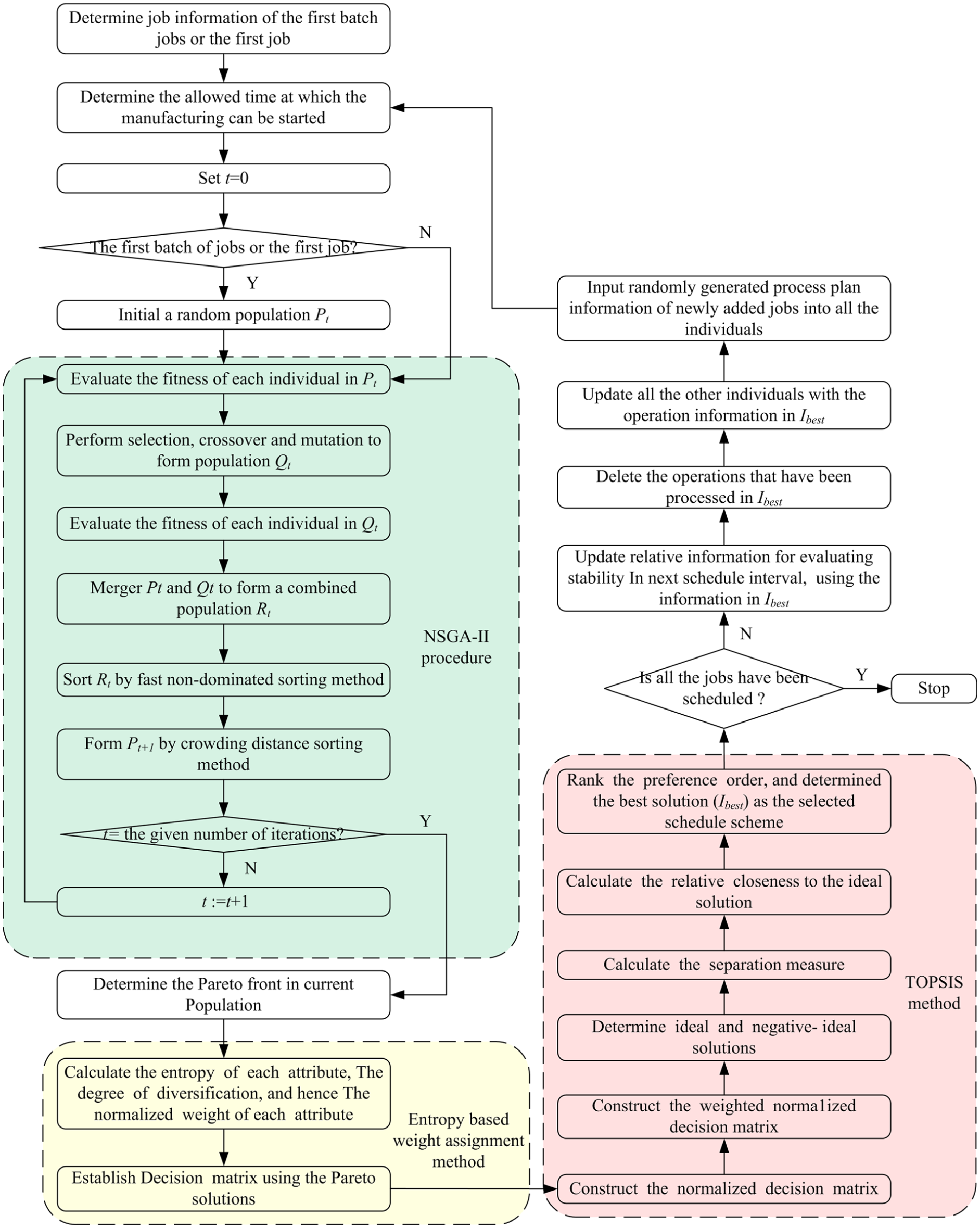
The flow chart of the dynamic scheduling strategy.

In event-driven rescheduling, the rescheduling point is the time at which a new job arrival occurs. In a real job shop environment, jobs arrive continuously over time, and newly added jobs will not be scheduled immediately. Instead, new jobs will be accumulated and considered for processing at the next rescheduling point. To make the problem correspond to the real-world situations as close as possible and make it manageable for analysis, we assume that all the newly added jobs during an interval can be added at one time at the forthcoming rescheduling point.

Experiments with discussions

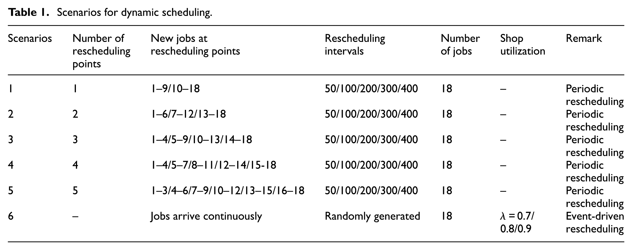
To study the effect of the factors and different scenarios on the performance of the manufacturing system, experiments are performed. We adopt the typical benchmark data proposed by Kim et al.¹⁵ 18 jobs will be processed by 15 machines. It has been extensively reported that a job shop with six machines is adequate to represent the complexity involved in a large dynamic job shop.³⁸ We consider both the periodic and event-driven rescheduling methods in our experiments with the scenarios listed in Table 1. Scenarios 1–5 are about periodic rescheduling, while the last scenario in Table 1 concentrates on event-driven rescheduling. In both dynamic rescheduling methods, the algorithm terminates when all the 18 jobs are finished (each case has the same total workload). All the experiments in this article are implemented in C++ and tested on a PC with Intel i5-3470 3.2 GHz CPU and 4 GB of RAM.

Table 1.

Scenarios for dynamic scheduling.

Scenarios	Number of rescheduling points	New jobs at rescheduling points	Rescheduling intervals	Number of jobs	Shop utilization	Remark
1	1	1–9/10–18	50/100/200/300/400	18	−	Periodic rescheduling
2	2	1–6/7–12/13–18	50/100/200/300/400	18	−	Periodic rescheduling
3	3	1–4/5–9/10–13/14–18	50/100/200/300/400	18	−	Periodic rescheduling
4	4	1–4/5–7/8–11/12–14/15-18	50/100/200/300/400	18	−	Periodic rescheduling
5	5	1–3/4–6/7–9/10–12/13–15/16–18	50/100/200/300/400	18	−	Periodic rescheduling
6	−	Jobs arrive continuously	Randomly generated	18	λ = 0.7/0.8/0.9	Event-driven rescheduling

Parameter setting

Parameter adjustments are performed to seek a good parameter setting since appropriate parameters are efficacious on the solution quality. The first scenario in Table 1 with rescheduling interval 200 is chosen to evaluate the parameters. Following values for the two parameters Pc (crossover probability) and Pm (mutation probability) are considered:

Pc: 0.6, 0.75, 0.9;

Pm: 0.05, 0.1, 0.15.

Thus, nine cases are defined as follows:

Case 1: Pc = 0.6, Pm = 0.05;

Case 2: Pc = 0.6, Pm = 0.1;

Case3: Pc = 0.6, Pm = 0.15;

Case 4: Pc = 0.75, Pm = 0.05;

Case 5: Pc = 0.75, Pm = 0.1;

Case 6: Pc = 0.75, Pm = 0.15;

Case 7: Pc = 0.9, Pm = 0.05;

Case 8: Pc = 0.9, Pm = 0.1;

Case 9: Pc = 0.9, Pm = 0.15.

We have run the algorithm 10 times on the considered scenario for the nine cases. The mean values of the Pareto solutions of all the combinations are plotted in Figure 6. This figure shows that we can obtain the best Pareto front that considers three criteria by setting Pc and Pm to 0.75 and 0.15, respectively. In other words, the parameter setting in Case 6 is adopted. In addition, the population and the number of iterations are set to 500 and 250, respectively.

Figure 6.

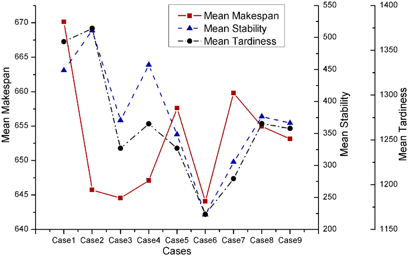
Mean values of Pareto solutions.

Periodic rescheduling

Pareto fronts for Scenario 1 with different interval lengths are presented in Figure 7(a). In Scenario 1, only one rescheduling is performed. With short rescheduling intervals, satisfactory makespan values can be ensured. However, the stability and the tardiness criteria deteriorate with short intervals. With a shorter rescheduling interval, there will be more unfinished operations, and hence, the probability of misalignments in starting times and the number of operations on a machine between the old schedule and the new schedule will increase. Moreover, the tardiness will increase with more unfinished operations although the interval is relatively short. On the contrary, the stability and the tardiness criteria have been greatly improved with long intervals although long intervals cause deteriorations in makespan values. In fact, with longer intervals, more operations can be processed in the current interval before the next rescheduling point, and it comes out that there are less unfinished operations. For the extreme case (Scenario 5) where there are more intervals, the corresponding plot is presented in Figure 7(b). It can be observed again that lengthening the rescheduling interval improves stability and tardiness criteria but deteriorates makespan measure. In addition, this also reflects that it is necessary to consider multiple objectives rather than single objective in dynamic IPPS problems because the makespan criterion conflicts with other criteria, such as the tardiness and the stability criteria, as reflected in Figure 7.

Figure 7.

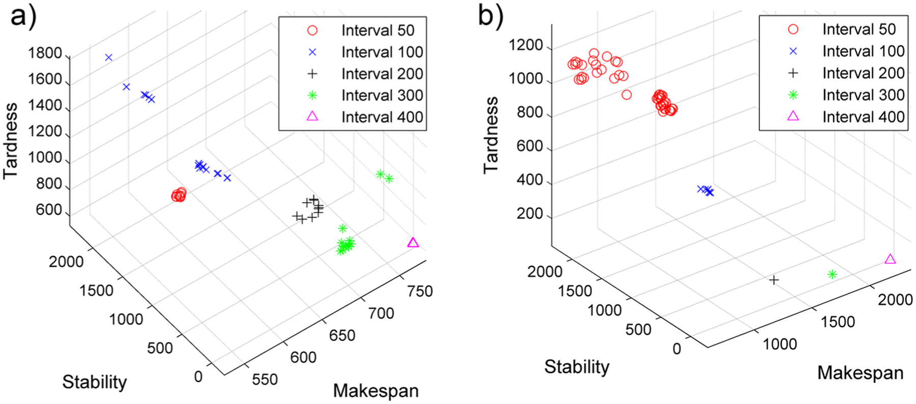
Pareto fronts of (a) Scenario 1 and (b) Scenario 5.

Figure 8(a) is the line chart of averages of the Pareto solutions of Scenario 1. As analyzed above, when the interval is less than 100, the makespan value seems acceptable. Due to the short interval length, only a few operations have the chance to be processed in the current interval. In such a case, most of the operations will be detained and processed in the next schedule. It can be observed that there is a slowdown of makespan value between the interval 200 and 300 in Figure 8(a). This indicates that most operations in the rescheduling interval can be finished without being rescheduled with such interval length. After that, the makespan value increases again. This is mainly brought on by a rise in interval length. We can also find that both stability and tardiness perceptibly receive improvements with the intervals that are larger than 300 according to Figure 8(a). For the mean stability in Figure 8(a), it decreases after an initial increase with a length between 50 and 100. We obtain the worst stability with an interval length 100, and after that, a sharp improvement occurs at the interval length 200. We study the reason behind the phenomenon. In the situation where the rescheduling interval is 50, only few operations are processed in an interval, and most operations should be rescheduled with different starting times. By narrowing the rescheduling interval, most of the unprocessed operations can be started on the same machine with almost the same starting times as the cases in the initial schedule. On the other hand, when the time interval is long enough, most of the operations can be finished in the current interval, and the stability criterion receives a large improvement. Based on such analysis, there exists a “peak point” at which the stability shows the worst performance. Thus, the optimal value of the rescheduling length in Scenario 1 should be set between 200 and 300. For Scenario 2, the optimal value of the rescheduling length is about 200 as shown in Figure 8(b). Different with the case in Figure 8(a), there is no increase in stability with a interval length between 50 and 100 in Figure 8(b). This objective receives no improvement both with interval lengths 50 and 100 because there are less new jobs for each interval in Scenario 2, and the peak point of the stability criterion in Figure 8(b) arises in advance. This conclusion is verified in Figure 8(c) and (d): with less and less new jobs in each interval, peak points in these figures appear in the leftmost regions. Hypothetically, if there were more newly added jobs in each interval, the peak point would appear later after the abscissa value 100. This left-shifting tendency of the peak point can also be observed in Figure 9(b)).

Figure 8.

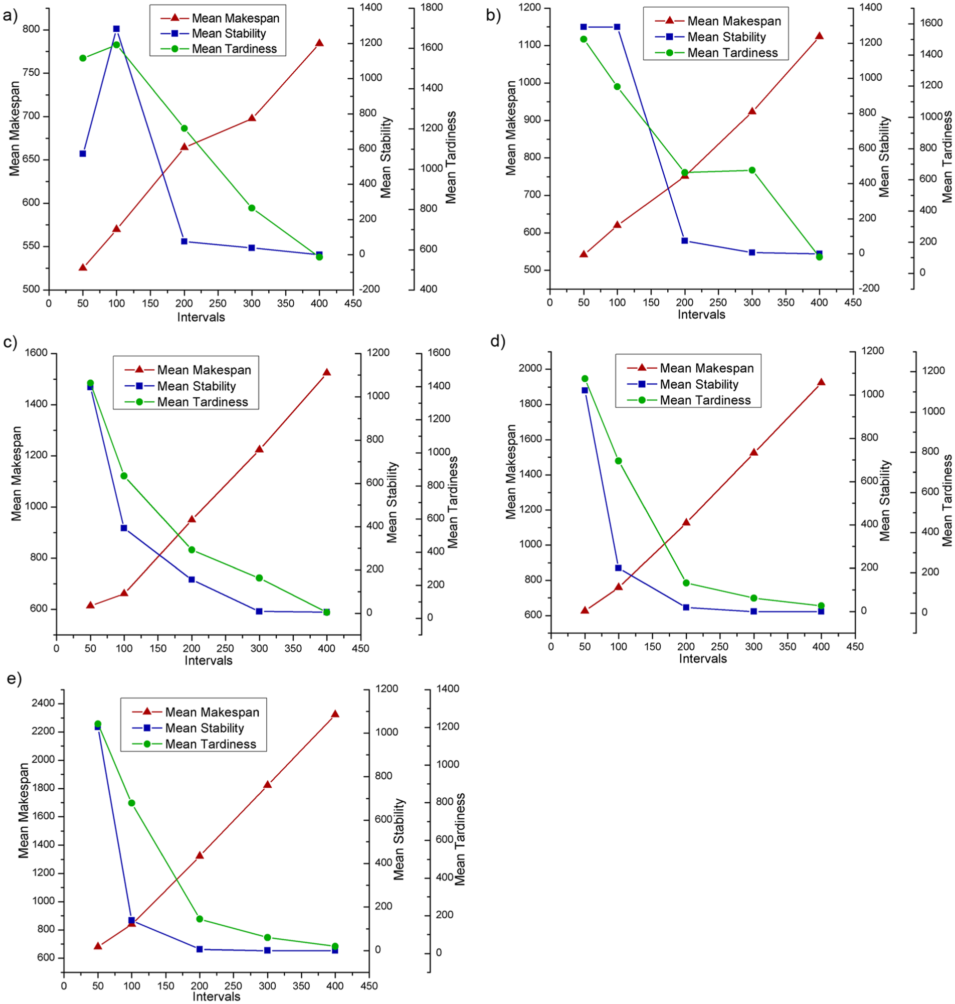
Averages of the Pareto solutions: (a) Scenario 1, (b) Scenario 2, (c) Scenario 3, (d) Scenario 4, and (e) Scenario 5.

Figure 9.

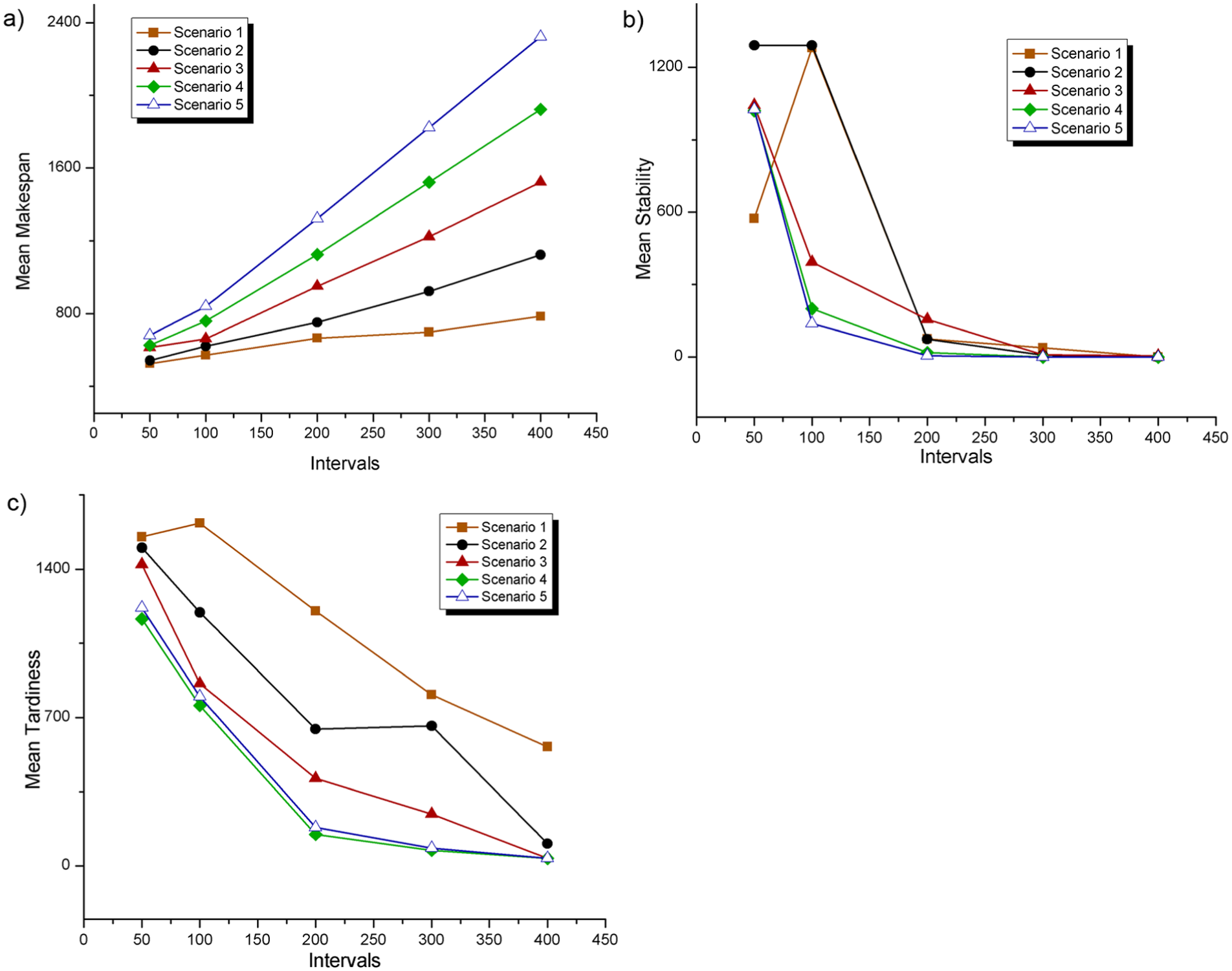
Averages of five scenarios with (a) makespan criterion, (b) stability criterion, and (c) tardiness criterion.

In Scenarios 3–5, due to fewer new jobs added in an interval, increasing the length of a rescheduling interval will lead to a dramatic increase in makespan. For the other two criteria in Figure 8(c)–(e), they both receive improvements with increasing interval length. Figure 9(a) gives the average makespan values of the Pareto solutions in five scenarios. Clearly, small rescheduling intervals will not lead to a dramatic increase in the makespan criterion; conversely, for a large rescheduling interval in a scenario which has frequent reschedulings (e.g. Scenario 5), the makespan increases dramatically. In general, the stability criterion is improved with the increasing rescheduling interval (Figure 9(b)). However, there are hardly any improvements for this criterion when the rescheduling interval is larger than 300 because the mean stability values are very close to 0 according to Figure 9(b). The tardiness criterion also improved with a large rescheduling interval according to Figure 9(c). Moreover, it receives more improvements in a scenario with more reschedulings. The reason behind this is that the unfinished jobs will have more chance to be finished in the coming intervals if there are more reschedulings. If there are less reschedulings (less intervals), unfinished jobs will certainly have less chance to be finished because they may be detained to the final interval, and hence the tardiness criterion may deteriorate.

Event-driven rescheduling

In this paradigm, the rescheduling is performed whenever a new job arrives (Scenario 6). Since the time between arrivals of jobs is controlled by the arrival rate λ as shown in equation (18), and the parameter λ is further determined by shop utilization η, we consider three statuses in a shop: a relatively idle status (η = 0.7), a normal state (η = 0.8), and a busy status (η= 0.9). Because a rescheduling point in this case is not known ahead, the study is realized by conducting some simulations where jobs arrive at random times for the entire scheduling horizon. We perform 10 runs for each status. Averages of Pareto fronts of 10 simulations are presented in Figure 10.

Figure 10.

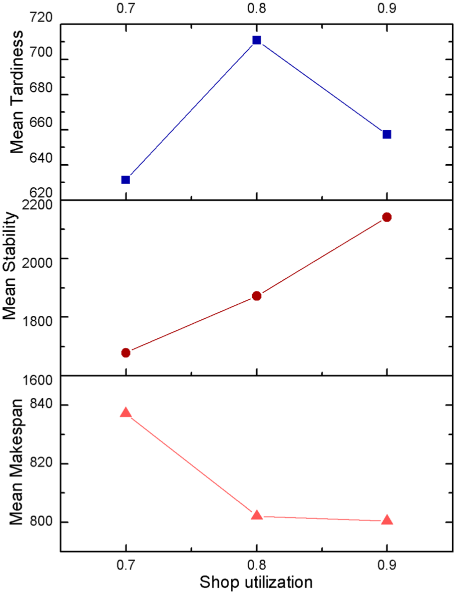
Averages of Pareto fronts of 10 simulations with three criteria.

A large shop utilization means shortening a rescheduling interval, and this will affect the stability criterion. As analyzed in section “Periodic rescheduling,” the peak point of the mean stability depends mainly on the number and the length of intervals and the number of new jobs in each interval. According to Figure 10, the mean stability shows a low performance when the interval is short (a large shop utilization) because frequent new job arrivals will result in more unfinished operations and this increases the risk of deteriorations of this criterion. Different with other two criteria, a busy status in a shop is helpful to the makespan criterion. A large shop utilization means shortening the interval between two job arrivals, and there are more operations to be detained to the last interval in such cases since less operations can be finished in a small interval. In such a case, the last interval is much longer than other intervals and more unfinished jobs will be finished in the last interval. This situation is very close to the deterministic scheduling case where there is only one interval without random job arrivals but competitive makespan values. Naturally, scheduling more unfinished jobs in the last interval will benefit the makespan criterion. For the tardiness criterion, it reaches the peak with a medium shop utilization (η = 0.8). With a small shop utilization, jobs are prone to be finished in a large interval, and hence, jobs are more likely to be finished before due dates. On the other hand, more operations will be detained to the last interval with a large shop utilization (a shorter interval length); as analyzed above, the makespan criterion will be improved and consequently this also benefits the tardiness criterion.

Conclusion

In this article, we study the characteristics of the IPPS problem with new job arrivals. A novel MILP model for the dynamic IPPS problem has been deduced. More importantly, a periodic and event-driven rescheduling framework is presented, and NSGA-II is applied to each scheduling interval with three criteria. Extensive experiments have been conducted, and the results show that the length of a scheduling interval, the number of new added jobs, and the shop utilization have an important influence on the efficiency of a manufacturing system. These resultant conclusions can be employed to guide real-life dynamic scheduling problems.

In this work, the processing time is deterministic. However, processing times are uncertain and subject to some probability distribution in real-world situations. Therefore, uncertain processing times can be further considered in the dynamic IPPS problem as a further research direction.

Footnotes

Appendix 1 Acknowledgements

The authors thank the anonymous referees for their insightful and valuable suggestions.

Declaration of conflicting interests

The author(s) declared no potential conflicts of interest with respect to the research, authorship, and/or publication of this article.

Funding

The author(s) disclosed receipt of the following financial support for the research, authorship, and/or publication of this article: This research is supported by the Funds for International Cooperation and Exchange of the National Natural Science Foundation of China (Grant No. 51561125002), National Natural Science Foundation of China (Grant Nos 51275190 and 51575211), and the Fundamental Research Funds for the Central Universities (HUST: 2014TS038).

References

Lian

Zhang

Shao

. Optimization of process planning with various flexibilities using an imperialist competitive algorithm. Int J Adv Manuf Tech 2012; 59: 815–828.

Mohammadi

Karampourhaghghi

Samaei

A multi-objective optimisation model to integrating flexible process planning and scheduling based on hybrid multi-objective simulated annealing. Int J Prod Res 2012; 50: 5063–5076.

Shao

Gao

Optimization of flexible process planning by genetic programming. Int J Adv Manuf Tech 2008; 38: 143–153.

Mohapatra

Nayak

Kumar

. Multi-objective process planning and scheduling using controlled elitist non-dominated sorting genetic algorithm. Int J Prod Res 2015; 53: 1712–1735.

Qiao

A cross-entropy-based approach for the optimization of flexible process planning. Int J Adv Manuf Tech 2013; 68: 2099–2110.

Phanden

Jain

Verma

Integration of process planning and scheduling: a state-of-the-art review. Int J Comp Integ M 2011; 24: 517–534.

Lian

Zhang

Gao

. Integrated process planning and scheduling using an imperialist competitive algorithm. Int J Prod Res 2012; 50: 4326–4343.

Dai

Tang

. Energy-aware integrated process planning and scheduling for job shops. Proc IMechE, Part B: J Engineering Manufacture 2015; 229: 13–26.

Kumar

Rajotia

Integration of process planning and scheduling in a job shop environment. Int J Adv Manuf Tech 2006; 28: 109–116.

10.

Amin-Naseri

Afshari

A hybrid genetic algorithm for integrated process planning and scheduling problem with precedence constraints. Int J Adv Manuf Tech 2012; 59: 273–287.

11.

Saygin

Kilic

SE.

Integrating flexible process plans with scheduling in flexible manufacturing systems. Int J Adv Manuf Tech 1999; 15: 268–280.

12.

Gao

WD.

Application of game theory based hybrid algorithm for multi-objective integrated process planning and scheduling. Expert Syst Appl 2012; 39: 288–297.

13.

Özgüven

Özbakır

Yavuz

Mathematical models for job-shop scheduling problems with routing and process plan flexibility. Appl Math Model 2010; 34: 1539–1548.

14.

Tan

Khoshnevis

A linearized polynomial mixed integer programming model for the integration of process planning and scheduling. J Intell Manuf 2004; 15: 593–605.

15.

Kim

Park

A symbiotic evolutionary algorithm for the integration of process planning and job shop scheduling. Comput Oper Res 2003; 30: 1151–1171.

16.

Shao

Gao

. Integration of process planning and scheduling – a modified genetic algorithm-based approach. Comput Oper Res 2009; 36: 2082–2096.

17.

Shao

Gao

. An effective hybrid algorithm for integrated process planning and scheduling. Int J Prod Econ 2010; 126: 289–298.

18.

Nowicki

Smutnicki

A fast taboo search algorithm for the job shop problem. Manage Sci 1996; 42: 797–813.

19.

Gao

Shao

XY.

An active learning genetic algorithm for integrated process planning and scheduling. Expert Syst Appl 2012; 39: 6683–6691.

20.

Lihong

Shengping

An improved genetic algorithm for integrated process planning and scheduling. Int J Adv Manuf Tech 2012; 58: 727–740.

21.

Zhang

Wong

TN.

An object-coding genetic algorithm for integrated process planning and scheduling. Eur J Oper Res 2015; 244: 434–444.

22.

Baykasoglu

Ozbakir

A grammatical optimization approach for integrated process planning and scheduling. J Intell Manuf 2009; 20: 211–221.

23.

McMahon

CA.

A simulated annealing-based optimization approach for integrated process planning and scheduling. Int J Comp Integ M 2007; 20: 80–95.

24.

Guo

Mileham

. Applications of particle swarm optimisation in integrated process planning and scheduling. Robot CIM: Int Manuf 2009; 25: 280–288.

25.

Shukla

Tiwari

Son

YJ.

Bidding-based multi-agent system for integrated process planning and scheduling: a data-mining and hybrid tabu-SA algorithm-oriented approach. Int J Adv Manuf Tech 2008; 38: 163–175.

26.

Wong

Leungy

Mak

. Integrated process planning and scheduling/rescheduling - an agent-based approach. Int J Prod Res 2006; 44: 3627–3655.

27.

Rangsaritratsamee

Ferrell

Jr Kurz

MB.

Dynamic rescheduling that simultaneously considers efficiency and stability. Comput Ind Eng 2004; 46: 1–15.

28.

Liu

Ong

KM.

Metaheuristics for minimizing the makespan of the dynamic shop scheduling problem. Adv Eng Softw 2005; 36: 199–205.

29.

Adibi

Zandieh

Amiri

Multi-objective scheduling of dynamic job shop using variable neighborhood search. Expert Syst Appl 2010; 37: 282–287.

30.

Fattahi

Fallahi

Dynamic scheduling in flexible job shop systems by considering simultaneously efficiency and stability. CIRP J Manuf Sci Technol 2010; 2: 114–123.

31.

Qiao

Process planning and scheduling integration with optimal rescheduling strategies. Int J Comp Integ M 2014; 27: 638–655.

32.

Gao

Shao

. Mathematical modeling and evolutionary algorithm-based approach for integrated process planning and scheduling. Comput Oper Res 2010; 37: 656–667.

33.

Deb

Pratap

Agarwal

. A fast and elitist multiobjective genetic algorithm: NSGA-II. IEEE T Evol Comput 2002; 6: 182–197.

34.

Bierwirth

A generalized permutation approach to job shop scheduling with genetic algorithms. Oper Res Spectr 1995; 17: 87–92.

35.

Tseng

HE.

Guided genetic algorithms for solving a larger constraint assembly problem. Int J Prod Res 2006; 44: 601–625.

36.

Hwang

C-L

Yoon

Multiple attribute decision making: methods and applications—a state-of-the-art survey. Berlin, Heidelberg: Springer, 1981, pp.52–140.

37.

Karsiti

Cruz

Jr Mulligan

Jr.

Simulation studies of multilevel dynamic job shop scheduling using heuristic dispatching rules. J Manuf Syst 1992; 11: 346–358.

38.

Chryssolouris

Subramaniam

Dynamic scheduling of manufacturing job shops using genetic algorithms. J Intell Manuf 2001; 12: 281–293.

A study on the impact of periodic and event-driven rescheduling on a manufacturing system: An integrated process planning and scheduling case

Abstract

Keywords

Introduction

Problem description

Mathematical modeling

NSGA-II-based solution methodology

Encoding and decoding

Genetic operators

Decision method

Objective function

Key parameters

The main framework

Experiments with discussions

Parameter setting

Periodic rescheduling

Event-driven rescheduling

Conclusion

Footnotes

Appendix 1

Acknowledgements

Declaration of conflicting interests

Funding

References