Sage Journals: Discover world-class research

Abstract

Flow forming as a precise locally plastic deformation is applied to fabricate thin-walled seamless tubes. Diametral growth as a dimensional defect that occurrs in a flow-formed tube is studied numerically and experimentally in this article. Flow forming of an AISI 321 steel tube is investigated using a finite element method with a dynamic explicit approach. The efficient parameters on the diametral growth are determined using experimental outcomes. The parameters considered are the thickness reduction (%), the feed rate of the roller (mm/min) and the roller nose radius (mm). Response surface methodology is employed to draw out a mathematical model of the diametral growth with regard to the significant parameters. The gained equation reveals that the thickness reduction is the most significant parameter and feed rate has the slightest effect on the diametral growth. The diametral growth increases with the rise in the thickness reduction and the roller nose radius and it leads to a decrease with a high value of feed rate. The innovation point of view is related to the fact that the high level of roller nose radius covers the efficiency of feed rate.

Keywords

Flow forming diametral growth response surface methodology

Introduction

Flow forming is a kind of metal spinning process to manufacture thin-walled high-precision and seamless tubular parts. In flow forming, a metal blank or pre-form is formed over a rotating mandrel. Thickness of the pre-form reduces when one or more rollers spin around their own axis and move axially along the rotating pre-form axis.

In recent years, many researchers have performed experimental and numerical studies on the flow forming process. Hayama and Kudo¹ developed a theory for forward and backward tube spinning and studied the diametral growth (DG) and strain rate in the deformation region and examined the evaluation of the diameteral preciseness of the flow-formed tubes. Kemin et al.² developed an elastic–plastic finite element (FE) model to simulate the tube spinning process in order to comprehend the properties of tube spinning and experimentally studied the DG. A FE model of tube spinning was presented by Xu et al.³ so as to categorize the deformation area in the axial, radial and tangential directions. Finite element method (FEM) results were in good agreement with the practical deformity condition and the experimental outcomes of Hayama and Kudo.¹ Hua et al.⁴ executed a practical spinning process of Hastelloy C alloy pre-form and simulated a three-dimensional (3D) elastic–plastic model. They showed that there are imperfections in the contact zone between the pre-form and the mandrel, such as bell-mouth, build-up, bulging and DG. Groche and Fritsche⁵ used flow forming as a recently developed technique to fabricate internally geared wheels with high precise dimensions.⁵

Davidson et al.⁶ investigated the quality of flow-formed annealed AA6061 tubular pre-form and evaluated the accrued imperfections. They used the Taguchi method to forecast the maximum elongation of flow-formed AA6061 tubular pre-form.⁷ Furthermore, they implemented a response surface methodology (RSM) tool to improve the surface roughness of flow-formed AA6061 tubular pre-form empirically.⁸

Parsa et al.⁹ evaluated the influences of the roller attack angle and feed rate on the flow formability of the forward flow-forming process. They showed that the S/L ratio (ratio of the contact length in the circumferential direction to the contact length in the longitudinal direction in the interface area between pre-form and roller) increases while the values of attack angle and feed rate increase. Debin et al.¹⁰ Simulated backward flow forming by the FEM and investigated the dependency of microstructure and texture to deformation records.

Roy et al.^11,12 accomplished experimental and numerical examinations on the flow-forming process and illustrated the contribution of the local equivalent plastic strain on the roller and mandrel. They investigated the correlation between the plastic strain and micro-indentation hardness. Furthermore, a generalized interpretation was developed considering the contact area between roller and pre-form during a single roller flow-forming operation.

Mohebi and Akbarzadeh¹³ investigated the local plastic deformation of AA 6063 alloy during a flow-forming process using only one roller. They attained that high shear strains happened in both the longitudinal and traverse direction of pre-form.

It is well known that the pre-form rotational speed, roller nose radius and attack angle, feed rate, and thickness reduction have important roles in specifying the characteristics of the flow-formed tube. A comprehensive article general study illustrated that there is no reported investigation about AISI 321 tubes and their quality aspects using the flow-forming principle. The purpose of this study is to predict the DG for flow-formed AISI 321 stainless steel tube using the FEM. The selected parameters affecting DG as the response are the thickness reduction, the feed rate and the roller nose radius. An experimentally validated FE model is used for performing parametric analysis. The utilized layout for numerical runs is based on Box-Behnken design as a RSM’s tool. Hence, the problem of getting optimized process parameters to achieve minimum DG of the flow-formed tube is endeavored in this investigation.

Three-roller forward flow forming

The three-roller forward flow-forming system is composed of a tubular pre-formed, three rollers and mandrel. The mandrel is a shaft with a morse end embedded on a headstock chuck. In the flow-forming process, the tubular pre-form is fastened on the mandrel shaft and pre-form flanged end fixed by a tailstock. The axial and radial movements of the pre-form are constrained and the pre-form rotation is achieved by mandrel rotation. The three rollers are arranged around the tubular pre-form symmetrically. The axes and motion directions of the mandrel and pre-form tube are aligned. When the flow-forming process begins, the mandrel and pre-form rotation speeds are equal and constant, and the rollers move from the flange end of rotated pre-form to the headstock chuck uniformly. Because of the friction between the rollers and pre-form interfaces, the rollers passively rotate with no, or slight, circumferential slip on pre-form.

The ratio of the wall thickness reduction of the pre-form to the initial wall thickness is named as the thickness reduction ratio.⁴ According to the volume constancy of the pre-form, the reduction in wall thickness leads to increase in the length of the pre-formed tube.⁷

Methodology

In the present work, a three-roller forward flow-forming process is simulated numerically using commercial FE software. The FE model is utilized to carry out simulation runs for each dictated set of input parameters of the RSM’s Box-Bankhen matrix. The influences of selected input parameters of the flow-forming process are then analyzed using analysis of variance (ANOVA) technique. Eventually, by applying the developed mathematical model of DG as the response, the optimum conditions are predicted and verified experimentally.

Experimental details

Tooling

A common numerically controlled lathe was used as a flow-forming machine. A three-roller tool apparatus was designed and built as shown in Figure 1. The apparatus was installed on the support of the lathe. Owing to the imposed pressure on flow-forming components, flow-forming tools (rollers and mandrel) must be made of high-strength steel. The mandrel morse end was fixed on lathe chuck and the pre-form was clamped on the mandrel. For roller shape determining, four rollers with different attack angle (15°, 20°, 25° and 30°) were manufactured.

Figure 1.

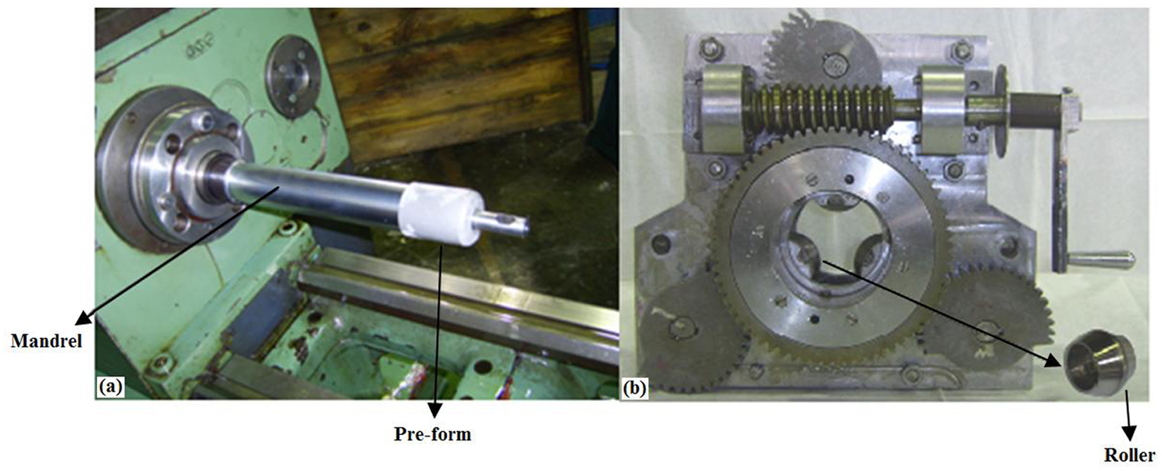
(a) Pre-form and mandrel installing on headstock chuck; (b) three-roller tool apparatus with a typical roller.

Pre-form

The AISI 321 stainless steel (DIN 1.4541) that has high strength and excellent corrosion resistance was used for experimental studies. The chemical composition of AISI 321 is given in Table 1. In the flow-forming process the dimensional preciseness of the final product is influenced by the dimensions and profile shape of the pre-form. The pre-form with an outer diameter of 50.5 mm and a length of 65 mm was manufactured by press forming of a circular blank with 1.5 mm of thickness and 139 mm of diameter. The initial pre-form and flow-formed tubes, after one pass, are shown in Figure 2.

Table 1.

Chemical composition of the AISI 321.

Material	Si	Ni	Mo	Mn	Ti	Cr	C	S	P	Fe
AISI 321	0.67	8.39	–	1.44	0.68	17.84	0.068	0.003	0.052	Bal

Figure 2.

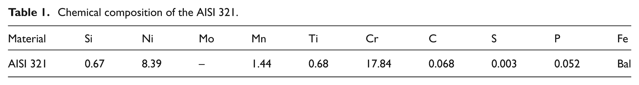
(a) Initial pre-form; and (b) flow-formed tube.

The hardness of the pre-formed tube was increased after each pass. Therefore, to decrease the hardness of the flow-formed tubes and prepare them for the next pass, the pre-forms were annealed at a temperature of 1050 °C for 20 min and then they were quenched in a vacuum furnace.

In this article, the DG of the flow-formed tubes as a response was measured with an ultrasonic wall thickness gage of ±0.001 mm accuracy.

Experimental conditions

In order to find out the main parameters affecting the DG of the flow-formed tube, preliminary tests were carried out. It was clear that the thickness reduction (%), the feed rate of the rollers (mm/min) and the roller nose radius (mm) have sensible effects on the DG. To obtain the favorite attack angle of the roller, the surface roughness of the flow-formed tubes produced with different attack angles of the roller (15°, 20°, 25° and 30°) were measured. Finally, the roller with attack angle of 25°, which produced a flow-formed tube with high surface finish (Ra = 0.9 $μ m$ ) was selected for the proposed experiments. Also, several experiments of the flow-forming process of AISI 321 stainless steel tubes indicated that the maximum deformation with high surface finish of the pre-form could be attained at a mandrel rotation speed of 350 r/min.

Simulation procedure

Material definition

The flow-forming process was applied to an AISI 321 stainless steel tube. Throughout flow forming there are large deformations, intensive rotation, complicated contact condition and nonlinearity encountered.¹⁴ The behavior of anisotropic plasticity is studied by using Hill’s yield criterion.¹⁵ Hill’s yield potential is an extension of the Von-Mises yield function used to model anisotropic metal plasticity. Holloman’s¹⁶ law was used to explain the stress dependence on effective plastic strain. Considering ASTM E8M-97, the material properties were determined from tensile tests that are provided in Table 2.

Table 2.

Mechanical properties of annealed AISI 321 stainless steel.

Material	$σ_{y}$ (MPa)	$σ_{u}$ (MPa)	E (GPa)	$ν$	$ρ$ (Kg/m3)	Elongation (%)	Hardness (HRB)	R₀	R₄₅	R₉₀
AISI 321	230	625	193	0.3	7830	53	86	0.88	0.92	0.91

The stress–strain curve of the pre-form material is presented in Figure 3. The roller and mandrel were assumed as 3D analytical rigid bodies and the pre-form was modeled as a deformable part.

Figure 3.

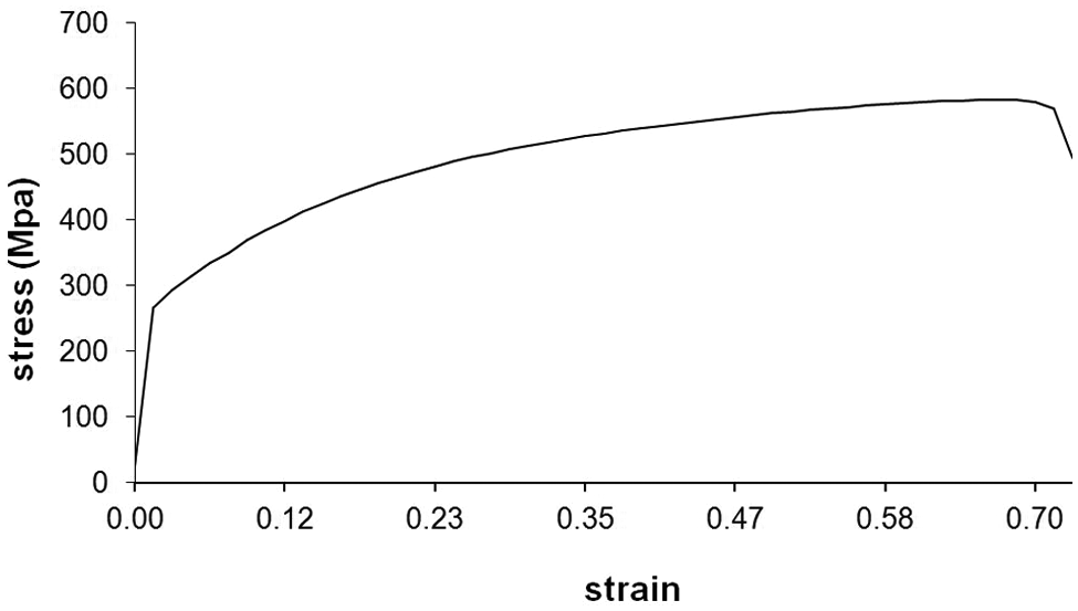
The engineering stress–strain curve of AISI 321.

Solving method

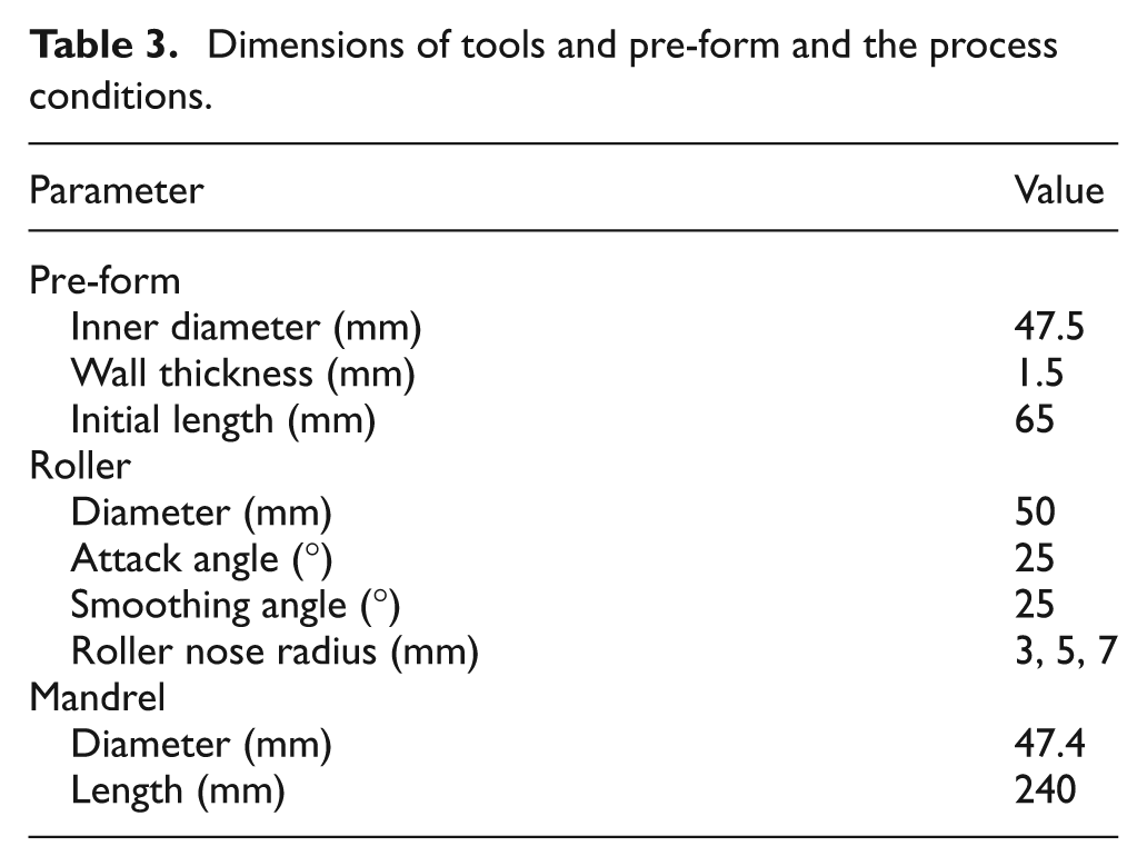
Elastic–plastic FEM is used in order to examine the influence of process parameters on the formability of the pre-form. Large plastic deformation occurs in the pre-form that is in contact with the rollers and mandrel in the tube spinning process. Owing to high non-linearity deformation behavior, both the geometrical and material non-linearity was noticed in the FEM analysis of tube spinning.⁴ Also, the explicit solving procedure was chosen.⁹ The geometrical dimensions of pre-form, rollers and mandrel are shown in Table 3.

Table 3.

Dimensions of tools and pre-form and the process conditions.

Parameter	Value
Pre-form
Inner diameter (mm)	47.5
Wall thickness (mm)	1.5
Initial length (mm)	65
Roller
Diameter (mm)	50
Attack angle (°)	25
Smoothing angle (°)	25
Roller nose radius (mm)	3, 5, 7
Mandrel
Diameter (mm)	47.4
Length (mm)	240

The tubular blank in the FE model of the process, which is presented in Figure 4, was meshed with a C3D8R element.¹⁰ Owing to large contact interfaces in the flow-forming process, surface to surface contact was applied in this model.⁹ Owing to using lubricant oil during the process, a frictionless interface mode was selected.¹³

Figure 4.

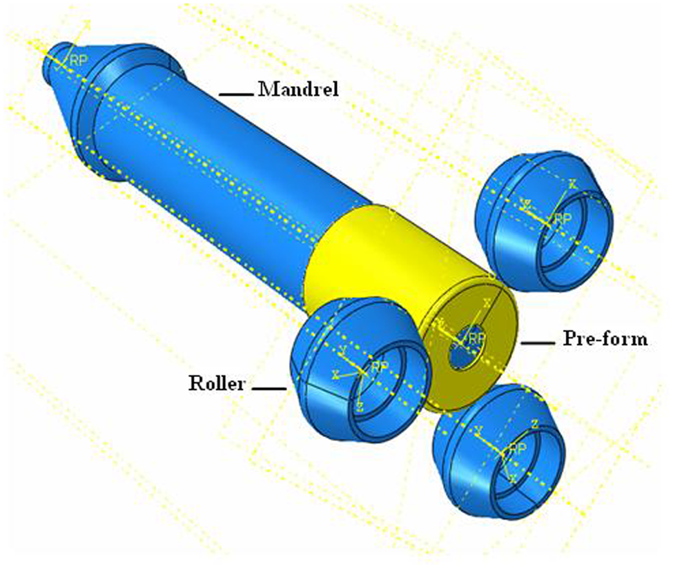
Schematic of forward flow forming by three rollers.

In the simulation presented here, the mass scaling element was selected so that the time consuming was decreased. Eventually, for the FE model validation, predicted thicknesses were compared with the experimental results. In addition, using experimentally acquired longitudinal strains of the flow-formed tube the credibility of the FE model was confirmed (Table 4). In Table 4 the comparison between experimental and the FEM longitudinal strains imply the error value between 2.1% and 8.8%. The given acceptable errors consider the validity of the model.

Table 4.

Obtained longitudinal strains of experimental and FEM in thickness reduction of 33 (%) and roller nose radius of 5 (mm).

Run no.	Rotational speed (r/min)	Feed rate (mm/min)	Longitudinal strain		Error (%)
			Exp.	FEM
1	300	45	0.22	0.21	4.5
2	300	60	0.24	0.225	6.2
3	300	75	0.235	0.23	2.1
4	350	45	0.225	0.21	6.6
5	350	60	0.245	0.225	8.1
6	350	75	0.25	0.24	4
7	400	45	0.225	0.205	8.8
8	400	60	0.24	0.22	8.3
9	400	75	0.265	0.245	7.6

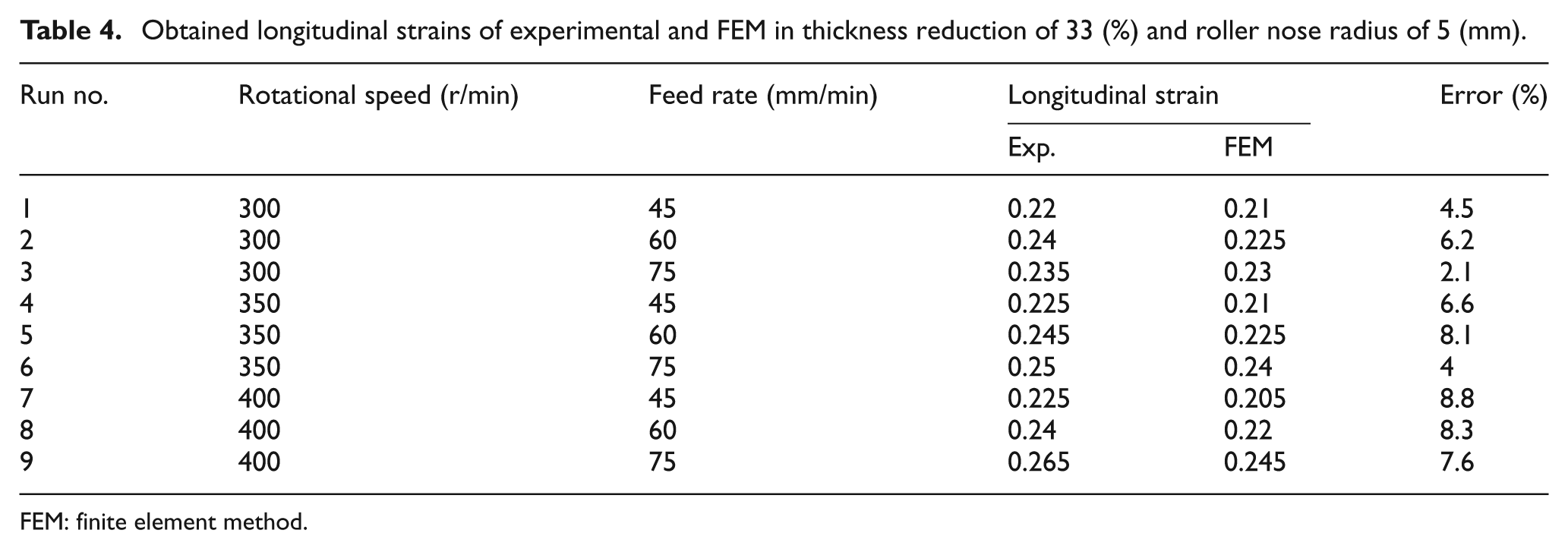
FEM: finite element method.

Design of experiments

The design of experiments (DOE) method is used to identify the planning of an experimental information gathering when the system is affected by a set of variable parameters.¹⁷ RSM, as a DOE tool, has recently noticed as an optimization technique in a numerical analysis area, was presented by Box and Wilson.¹⁸

The RSM is a type of optimization method that uses a function called a response surface to predict the optimum status. A response surface is applied as a function that approximates a response related an to independent variable and state quantities of response using several analyses of DOE results. With the RSM, optimal conditions are first determined, and then a response surface is created between the design variables and objective functions considering constraint condition limits. By using the created response surface, an optimal solution can be attained with a conventional optimization technique (Figure 5).

Figure 5.

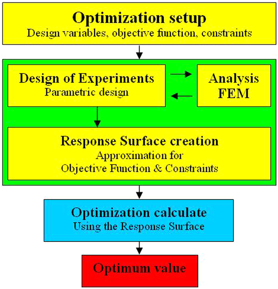
Response surface methodology.

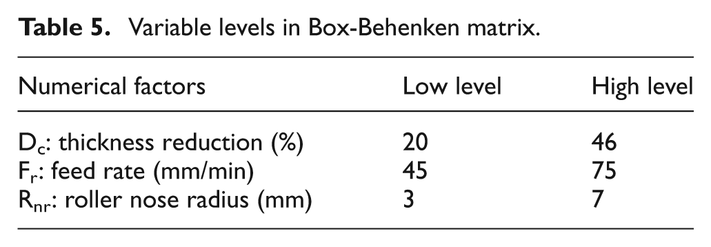
In this article, the Box-Behnken matrix dictates the experimental layout in 17 sets of runs for evaluation of three numerical factors and quantifying the mathematical model of DG attained by flow forming of AISI 321 steel tube. The variable levels of the Box-Behenken matrix are presented in Table 5.

Table 5.

Variable levels in Box-Behenken matrix.

Numerical factors	Low level	High level
D_c: thickness reduction (%)	20	46
F_r: feed rate (mm/min)	45	75
R_nr: roller nose radius (mm)	3	7

The Box-Behnken design matrix displays factors levels in the experimental layout (Table 6). This matrix was dictated for a layout run of the FE models.

Table 6.

Experimental layout for the Box-Behnken matrix.

FE run no.	Parameters			FE: DG ( $μ m$ )
	D_c	F_r	R_nr
1	33	60	5	165
2	20	60	7	75
3	33	60	5	165
4	46	60	7	175
5	33	45	7	162
6	20	60	3	51
7	33	60	5	165
8	33	75	3	101
9	46	75	5	156
10	33	75	7	161
11	33	45	3	156
12	46	60	3	138
13	20	45	5	78
14	46	45	5	186
15	20	75	5	67
16	33	60	5	165
17	33	60	5	165

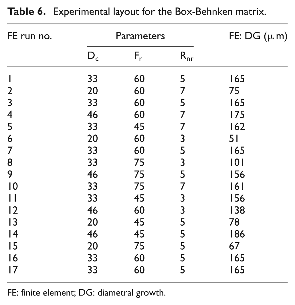
FE: finite element; DG: diametral growth.

Results and discussion

With the Box-Behnken design methodology, major and reciprocal effects of parameters on response function can be easily assessed. The consequential factors in the regression model can be appraised by performing ANOVA.¹⁹ It is inevitable to have an explanation about different statistical practical terms in this study. The definition for each term is shown in the Appendix.

ANOVA and developed mathematical model

The ANOVA was applied to investigate the influences of the input factors on the DG. The model summary statistics of different sources are given in Table 7. Model summary statistics composed of the R-squared, the adjusted R-squared, the predicted R-squared and the predicted residual error sum of squares (PRESS). Where R² is a gage of the amount of deviation around the mean explained by the model and adjusted R² is the R-squared adjusted for the number of terms in the model proportionate to the number of points in the design matrix. Predicted R² is a gage of the amount of degree of diversity in new data explained by the model. It displays that the quadratic model with maximum adjusted R² and predicted R² values and minimum PRESS value is the best model recommend as asuitable case. Thus, for advance analysis, this model was suggested.⁸

Table 7.

Model succinct statistics.

Model	Standard deviation	R²	Adjusted R²	Predicted R²	PRESS
Linear	26.28	0.7065	0.6388	0.5082	15052.05
2FI	28.50	0.7347	0.5755	0.1460	26135.83
Quadratic	2.5	0.9986	0.9967	0.9771	700.00 Suggested

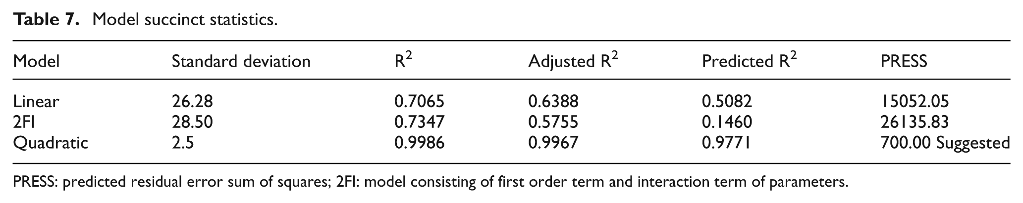
PRESS: predicted residual error sum of squares; 2FI: model consisting of first order term and interaction term of parameters.

Table 7 gives the ANOVA of the reaction surface model for the DG. ANOVA is used to determine the importance of the effects of the model terms of the response. If the value of “Prob > F” for the model is less than 0.05, the ANOVA proves the adequate accuracy of quadratic model.²⁰ In this case the model is worthwhile because it signifies that the terms in the model have an important effect on the response. The significance of each coefficient can be obtained by the “P-value”, which is listed in Table 8. In this case A, B, C, AB, AC, BC, A², B² and C² are significant model terms.

Table 8.

ANOVA for response surface quadratic model (response: DG).

Source	Sum of squares	DF	Mean square	F-value	P-value (probability > F)
Model	30562.01	9	3395.78	543.32	< 0.0001
A – thickness reduction (%)	18432.00	1	18432.00	2949.12	< 0.0001
B – feed rate	1176.13	1	1176.13	188.18	< 0.0001
C – roller nose radius	2016.13	1	2016.13	322.58	< 0.0001
AB	90.25	1	90.25	14.44	0.0067
AC	42.25	1	42.25	6.76	0.0354
BC	729.00	1	729.00	116.64	< 0.0001
A²	6486.58	1	6486.58	1037.85	< 0.0001
B²	67.37	1	67.37	10.78	0.0134
C²	1077.89	1	1077.89	172.46	< 0.0001
Residual	43.75	7	6.25
Core. total	30605.76	16

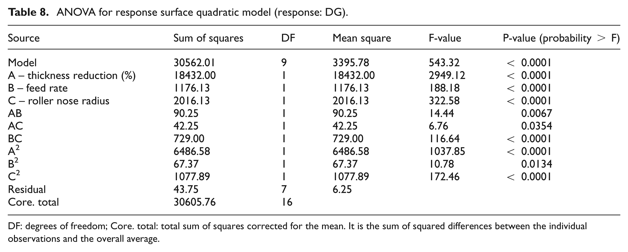
DF: degrees of freedom; Core. total: total sum of squares corrected for the mean. It is the sum of squared differences between the individual observations and the overall average

The “Model F-value” of 543.32 shows the significance of the model, because the “P-value” of 0.0001 implies that there is a possibility of 0.01% that a “model F-value” could transpire owing to noise.²¹

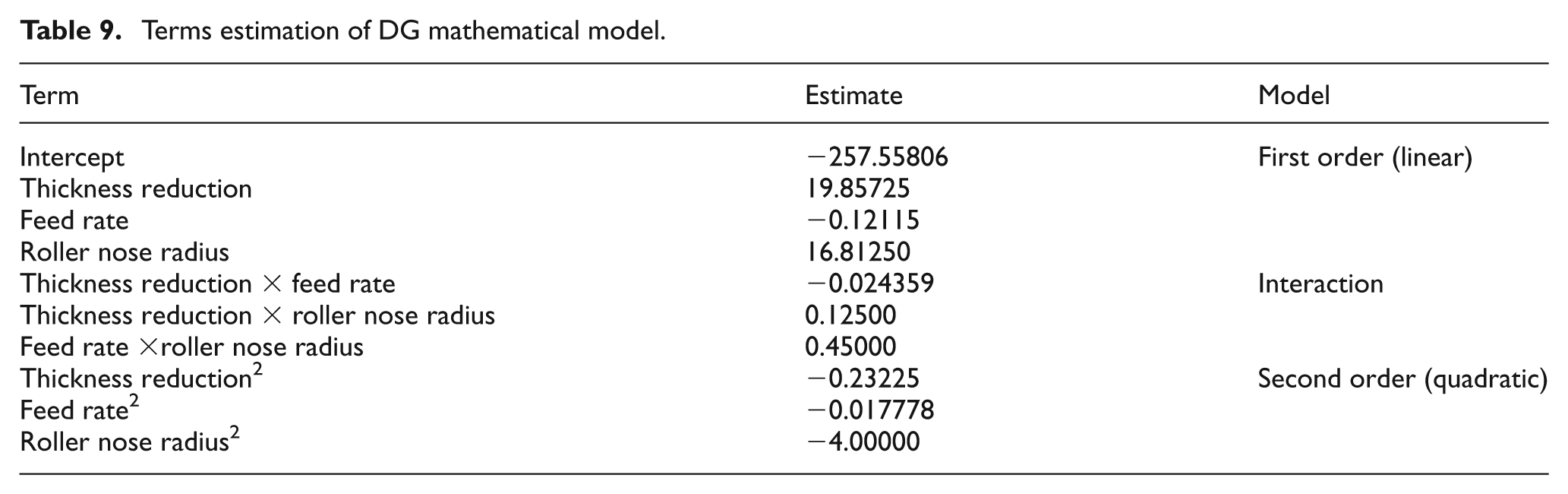
The comparison of the “F-value” of the parametric sources indicates that the thickness reduction is the most significant parameter influencing the DG. After the thickness reduction, the roller nose radius and the feed rate have more influence on DG, respectively. The estimated terms as coefficients of the DG mathematical model are given in Table 9.

Table 9.

Terms estimation of DG mathematical model.

Term	Estimate	Model
Intercept	−257.55806	First order (linear)
Thickness reduction	19.85725
Feed rate	−0.12115
Roller nose radius	16.81250
Thickness reduction × feed rate	−0.024359	Interaction
Thickness reduction × roller nose radius	0.12500
Feed rate ×roller nose radius	0.45000
Thickness reduction²	−0.23225	Second order (quadratic)
Feed rate²	−0.017778
Roller nose radius²	−4.00000

Confirmation of analysis

The computed values of regression are given in Table 10. High resulted coefficient of regression value (R² = 0.9986) demonstrated the competency of the represented model. The R² value varies between 0 and 1. It leads to an increase with decline in the residual errors. To signify the competency of analysis, adjusted coefficient of regression (Adj. R²) is utilized when the number of variables increases. In this model, a high-resulted coefficient of regression value (Adj. R² = 0.9967) illustrates the competency of the model.

Table 10.

Calculated value of regression and accuracy of the model.

Standard deviation	2.50
Mean	137.12
Coefficient of variation %	1.82
PRESS	700.00
R-squared	0.9986
Adj-squared	0.9967
Pred R-squared	0.9771
Adequate precision	71.711	Desire > 4

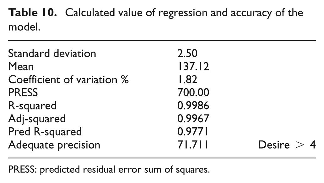
PRESS: predicted residual error sum of squares.

Adequate precision represents the competency of the model. When it is over 4, indicates the model significance level. From Table 10 it is clear that the adequate precision value of 71.711 is considerable. The predicted R² value of 0.9771 implies that the model could explain 97% of the variability in predicting new observations.

The residuals, which are the differences between the corresponding actual responses and the predicted responses, are reviewed using the plot of the residual errors and internally studentized residuals plot in contrast to predicted response. The competency plots of the model are shown in Figure 6.

Figure 6.

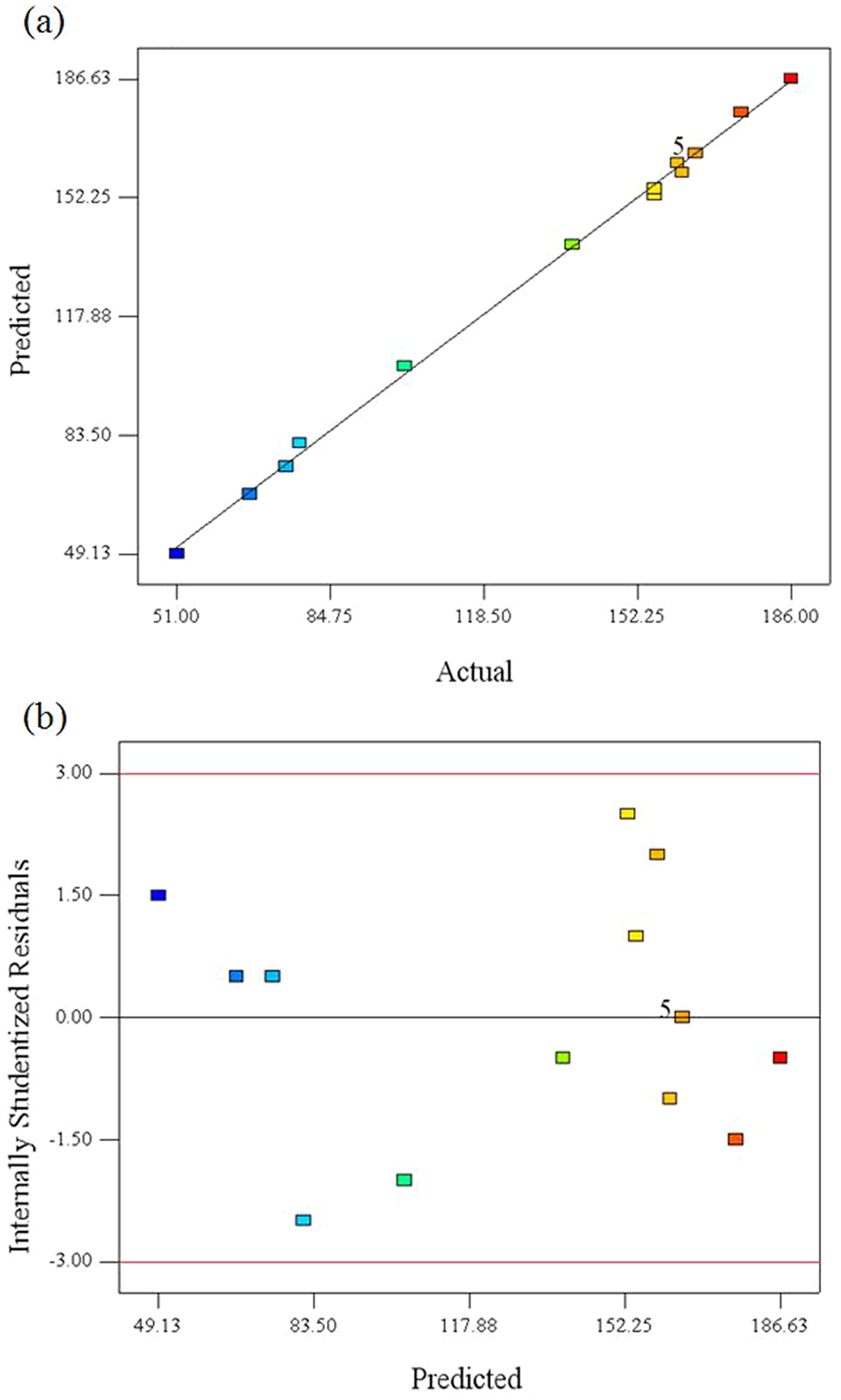
Diagnostic contour plots: (a) the predicted versus actual responses of DG; (b) the residuals versus predicted responses of DG.

The points on the predicted versus actual response plot (Figure 6(a)) lie on a straight line, so the model is qualified. Also in the qualified model, the plot of the residuals versus the predicted responses (Figure 6(b)) should contain no obvious pattern.²² Hence, it is clear that the model is qualified.

DG and 3D graphs

Imperfections and related failures that occurred on flow-forming tubes can be classified as micro cracks, DG, ovality, fish scaling and fracture bursting.²³ In fact, the material in front of the roller has a tendency to accumulate and form a heap on the surface. The tangential tensile strain that causes DG during the forming process is the major parameter in influencing the spinnability.²⁴ DG, as a dimentional imperfection, was found on flow-formed AISI 321 stainless steel tubes in this experimental study. Predicted wall thickness is not as much as the real amount of it. It is owing to the happened spring-back on the deformation zone. A large amount of depth of cut merged with low feed rates makes a large amount of DG. The DG is another way of adjusting material flow by the materials outside the deformation area. It should be noticed that materials at the end of the tube have a DG instead of pile-up.¹³ It was found that the DG rises by decreasing the feed rate and increasing the depth of cut. Figure 7 reveals that the pile-up on the flow-formed tube becomes greater by raising the thickness reduction.

Figure 7.

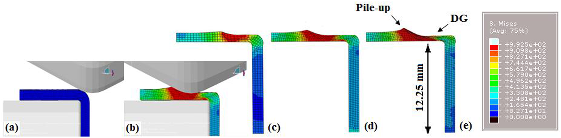
Section views of the FE model: (a) before, (b) after flow forming, and a flow-formed tube in thickness reduction of (c) 20%, (d) 33% and (e) 46%.

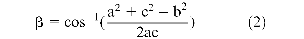
Material flow can be appraised using the contact ratio (S/L), in which L is the longitudinal direction and S is the circumferential direction of the contact area between the roller and the tube. The values of L and S can be computed using geometrical calculations as follows.²⁵

S = R_{r} β

(1)

where $β$ is expressed by

β = {cos}^{- 1} (\frac{a^{2} + c^{2} - b^{2}}{2 ac})

(2)

where a, b and c are defined as

a = R_{r} + T_{fi} + R_{m}

(3)

c = R_{r}

(4)

b = R_{m} + T_{fi} + Ftan α

(5)

L ≅ (\frac{T_{in} + T_{fi} + 2}{tan α + F})

(6)

where α is the attack angle, R_r is the roller radius, R_m is the mandrel radius, T_in is the final thickness, T_fi the final thickness, F the feed rate, and T the thickness difference.

The instability and related imperfections founded in flow forming are foreseeable by using the S/L ratio (Figure 8). DG is a function of the ratio of the circumferential contact length S to the longitudinal contact length L. DG is low in the high value of the S/L ratio and the smaller S/L ratio leads to form considerable DG.

Figure 8.

Contact area between tube and roller of FE model.

Figures 9, 10 and 11 give the 3D surface graphs for the predicted DG results. From Figure 9 it is clear that DG rises with an increase in thickness reduction and also rises with the combination of high value depth of cut with low feed rates owing to the reduction of S/L ratio. In addition, the feed rate of the roller has no considerable influence on DG in lower thickness reduction levels. However, in higher levels of thickness reduction the DG increases with a reduction in the feed rate. Consequently, interaction effects of thickness reduction and feed rate on flow-formed tubes are considerable.

Figure 9.

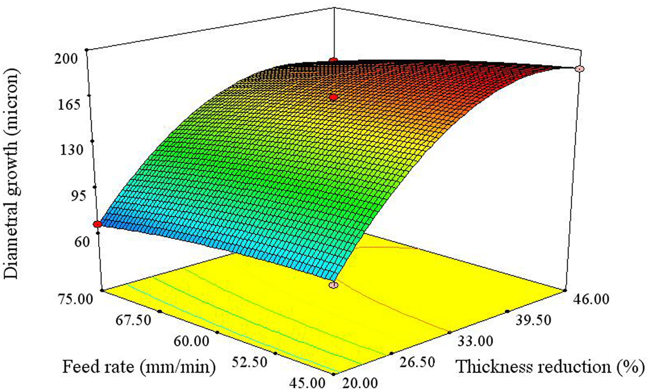
The effects of feed rate and thickness reduction on the DG on the constant roller nose radius (5 mm).

Figure 10.

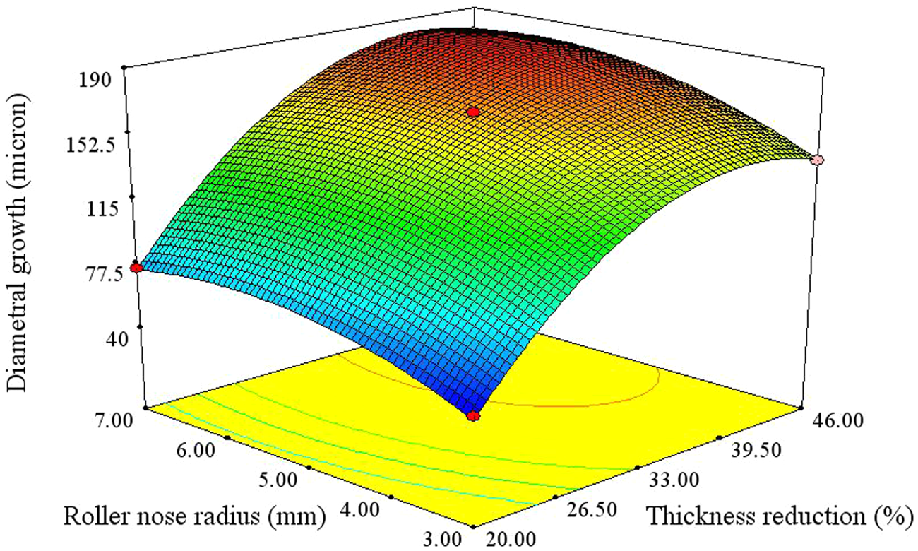
The effects of the roller nose radius and thickness reduction on the DG in the constant feed rate (60 mm/min).

Figure 11.

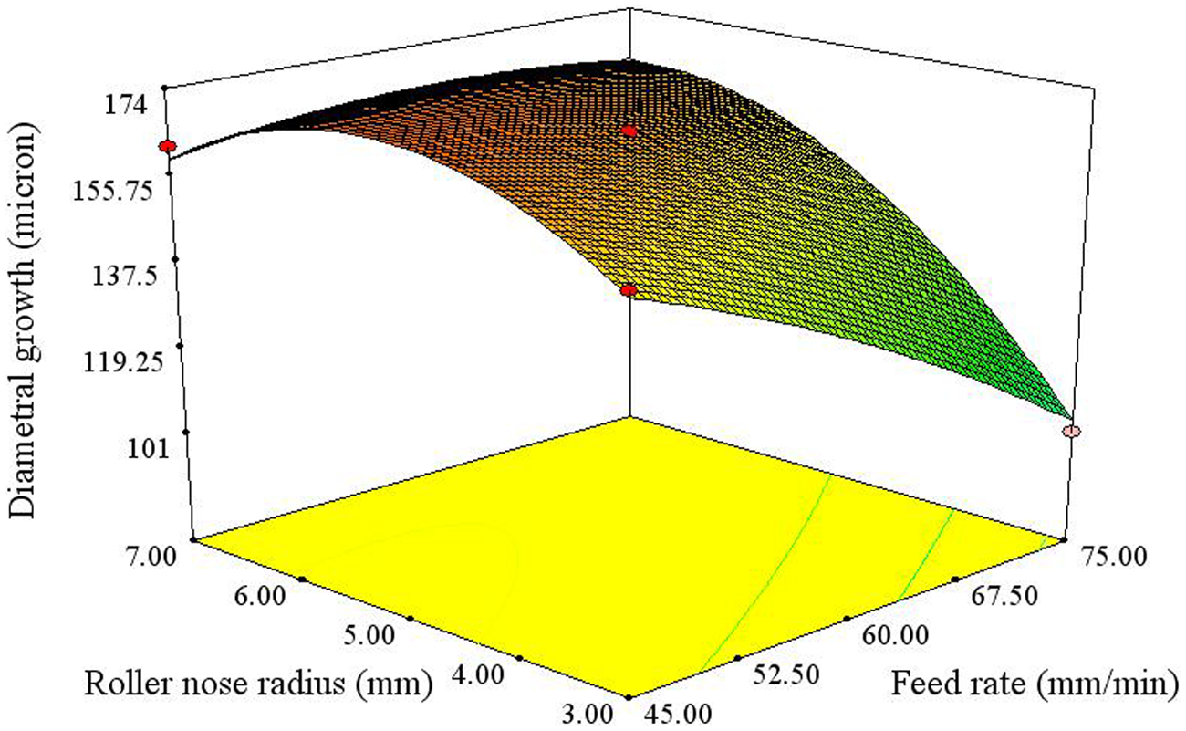
The effects of roller nose radius and feed rate on the DG in the constant thickness reduction (33%).

The interaction effects of the roller nose radius and thickness reduction on the DG are presented in Figure 10. According to equations (1)–(6), the combination of higher levels of roller nose radius and thickness reduction, causes the lower S/L ratio. It is obvious that the reduction of the S/L ratio results in maximum DG. Consequently, in lower levels of roller nose radius and thickness reduction the DG has the minimum value.

There is a substantial occurrence in interaction effects of the roller nose radius and feed rate (Figure 11). At higher levels of roller nose radius, the effect of feed rate is not considerable. The contact area between the rollers and pre-form is expanded by increasing the value of the roller nose radius. Afterwards, the plastic deformation process is influenced. The high level of the roller nose radius compensates the effects of feed rate when the mandrel rotational speed is constant.

Verification experiment

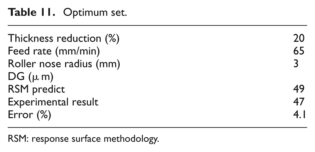
The RSM model predicted the minimum value of DG (Table 11). In order to approve the exactness of the advanced model, a confirmation test was carried out. The computed error has an authorized value. So, the developed mathematical model of the DG has the competency to predict the DG values for any layout of experiments consisting of the thickness reduction, the feed rate and the roller nose radius.

Table 11.

Optimum set.

Thickness reduction (%)	20
Feed rate (mm/min)	65
Roller nose radius (mm)	3
DG ( $μ m$ )
RSM predict	49
Experimental result	47
Error (%)	4.1

RSM: response surface methodology.

Conclusion

A coupled set of experiments and FE simulations were conducted to predict the DG in a three-roller flow-forming process. The effects of the process parameters on dimensional quality of the flow-formed AISI 321 tube were quantified by applying RSMs Box-Bankhen design. The following conclusions may be drawn by outcomes.

Using a FEM and DOE coupled set is very useful to cost saving in experiments and reducing the computational time consuming FE analyses.

The ANOVA estimations revealed that the thickness reduction was the most significant parameter influencing the DG. After the thickness reduction, the roller nose radius and the feed rate have more influences on DG, respectively.

It revealed that the minimum value of DG occurs in the thickness reduction = 20%, feed rate = 60 mm/min and at the minimum value of the roller nose radius.

The maximum value of DG was attained in high levels of thickness reduction and roller nose radius.

In lower thickness reduction levels and higher roller nose radius, the feed rate of the roller has an insensible effect on DG.

The contact interface area in the deformation zone and S/L ratio can perform a criterion for predicting the quality of dimensional defect in the flow-forming process.

The confirmability between RSM prediction and experimental results verified the adequate precision of the FEM model.

Footnotes

Appendix

Funding

This research received no specific grant from any funding agency in the public, commercial, or not-for-profit sectors.

References

Hayama

Kudo

. Analysis of diametral growth and working forces in tube spinning. Bull JSME 1979; 22: 776–784.

Kemin

Zhen

Yan

. Elasto-plastic FEM analysis and experimental study of diametral growth in tube spinning. J Mater Process Technol 1997; 69: 172–175.

Zhang

. 3D rigid plastic FEM numerical simulation of tube spinning. J Mater Process Technol 2001; 113: 710–713.

Hua

Yang

Zhang

. Three-dimensional finite element analysis of tube spinning. J Mater Process Technol 2005; 168: 68–74.

Groche

Fritsche

. Application and modelling of flow forming manufacturing processes for internally geared wheels. J Mater Process Technol 2006; 46: 1261–1265.

Davidson

Balasubramanian

Tagore

GRN

. An experimental study on the quality of flow-formed AA6061 tubes. J Mater Process Technol 2008; 203: 321–325.

Davidson

Balasubramanian

Tagore

GRN

. Experimental investigation on flow-forming of AA6061 alloy-A Taguchi approach. J Mater Process Technol 2008; 200: 283–287.

Davidson

Balasubramanian

Tagore

GRN

. Surface roughness prediction of flow-formed AA6061 alloy by design of experiments. J Mater Process Technol 2008; 202: 41–46.

Parsa

Pazooki

AMA

Nili Ahmadabadi

. Flow-forming and flow formability simulation. Int J Adv Manuf Technol 2009; 43: 463–473.

10.

Debin

Guoping

Wenchen

. Deformation history and the resultant microstructure and texture in backward tube spinning of Ti–6Al–2Zr–1Mo–1V. J Mater Process Technol 2009; 209: 5713–5719.

11.

Roy

Klassen

Wood

. Evolution of plastic strain during a flow forming process. J Mater Process Technol 2009; 209: 1018–1025.

12.

Roy

Maijer

Klassen

. Analytical solution of the tooling/workpiece contact interface shape during a flow forming operation. J Mater Process Technol 2010; 210: 1976–1985.

13.

Mohebbi

Akbarzadeh

. Experimental study and FEM analysis of redundant strains in flow forming of tubes. J Mater Process Technol 2010; 210: 389–395.

14.

Sun

Lee

. Comparison of implicit and explicit finite element methods for dynamic problems. J Mater Process Technol 2000; 105: 110–118.

15.

Hill

. The mathematical theory of plasticity. Oxford: Clarendon Press, 1950.

16.

Holloman

. Tensile deformation. Transition of the American Institute Mining. Metall Petroleum Engng 1949; 16: 268–290.

17.

Montgomery

. Design and analysis of experiments. 4th ed. New York: John Wiley, 1997.

18.

Box

GEP

Wilson

. On the experimental attainment of optimum condition. J Royal Statistical 1951; 13: 1–45.

19.

Box

GEP

Hunter

. Statistics for experiments – An introduction to design, data analysis and modeling. New York: Wiley, 1978.

20.

Cansee

Uriyapongson

Watyotha

. Amphoteric starch in simultaneous process preparation with Box-Behnken design for optimal conditions. Am J Applied Sci 2008; 52(11): 1535–1542.

21.

Edrissi

Razzaghiasl

. Complexation of iron with piroxicam – evaluation via response surface methodology. Acta Chim Slov 2007; 54: 825–833.

22.

Noordin

Venkatesh

Sharif

. Application of response surface methodology in describing the performance of coated carbide tools when turning AISI 1045 steel. J Mater Process Technol 2004; 145: 46–58.

23.

Rajan

Narsimhan

. An investigation of the development of defects during flow forming of high strength thin wall steel tubes. ASM J Pract Failure Anal 2001; 5: 69–76.

24.

. Thickness reduction spinning of the thin-walled cylinder with inner stiffness. In: Proceedings of the 4th international conference of rotary forming, International Academic Publishers, Beijing, China, October 17–21, 1989; 97–102.

25.

Jahazi

Ebrahimi

. The influence of flow-forming parameters and microstructure on the quality of a D6ac steel. J Mater Process Technol 2000; 103: 362–366.

Flow forming optimization based on diametral growth using finite element method and response surface methodology

Abstract

Keywords

Introduction

Three-roller forward flow forming

Methodology

Experimental details

Tooling

Pre-form

Experimental conditions

Simulation procedure

Material definition

Solving method

Design of experiments

Results and discussion

ANOVA and developed mathematical model

Confirmation of analysis

DG and 3D graphs

Verification experiment

Conclusion

Footnotes

Appendix

Funding

References