Sage Journals: Discover world-class research

Abstract

Originally developed for biomedical applications and diagnosis, optical coherence tomography (OCT) has recently been demonstrated to be a powerful non-destructive and non-invasive measurement method for detecting defects in glass-fiber reinforced polymer composites. While previous studies have focused mainly on the use of OCT in the analysis of thermoset composites, we were able to show in offline experiments that OCT can be used to quickly detect typical defects (e.g., dry fiber regions, gaps and fiber breakage) in thermoplastic unidirectional (UD) tapes at high resolution. To investigate the applicability of OCT to inline monitoring, we advanced our previously published approach in two major steps: First, we incorporated the OCT system into an industrial-scale UD-tape production line, and derived optimal settings for inline detection of dry region defects from a comprehensive design of experiments (DoE) to find an optimal balance between accuracy and data size for a stationary tape sample by varying A-scan sampling rate, A-scan averaging and OCT transverse travel velocity. Second, using these optimal settings, we went on to investigate moving tapes over a range of industrially relevant take-off speeds. Microscopy was used for validation in both cases. We developed a fast and robust statistical analysis of B-scans that visualizes the quality of full cross-sections in an interpretable manner for potential use in a real-time setting. Within an industrially relevant production speed range of up to 15 m/min, we are thus now able to investigate 120 mm wide (and potentially wider) UD tapes inline at a transverse resolution of 22 µm, producing only 21 MB of data per measurement.

Keywords

Thermoplastic unidirectional tapes optical coherence tomography unidirectional glass-fiber reinforced thermoplastics inline defect detection non-destructive testing

Introduction

The European Commission has adopted a set of proposals to make the EU’s climate, transport, energy, and taxation policies ready for the reduction, by 2030, of greenhouse gas emissions by at least 55% compared to 1990 levels.¹ In the transport sector in particular, a reduction in the mass to be carried will result in significantly lower fuel consumption and thus lower emissions and contribute to achieving these goals. In this context, composites made from continuous-fiber reinforced polymers with their excellent strength-to-weight and stiffness-to-weight ratios will play an important role. While composites were originally based on thermosets, we have observed a trend towards thermoplastic materials in recent years.²

In the manufacturing of thermoset-based composites, fibers are typically impregnated with a non-polymerized material, usually a low-molecular-weight resin that has very low viscosity, penetrates easily into the fiber carpet, and thus facilitates efficient impregnation.³ Polymerization and crosslinking are initiated and promoted by curing agents and catalysts during the curing process, which results in a hard but brittle polymer matrix. Since this chemical crosslinking reaction is irreversible, thermosets are difficult to recycle mechanically.⁴ Thermoplastics, in contrast, are fully polymerized at the time of impregnation. Consequently, they can be produced in highly automated processes with reduced cycle times, provide high design flexibility, and allow functional integration. Compared to their thermoset counterparts, however, thermoplastic materials exhibit higher viscosities, which makes the impregnation process more complex, requiring higher processing temperatures and more energy.

Unidirectional (UD) fiber-reinforced thermoplastic tapes are becoming increasingly important as semi-finished products because – with minimal weight – they have excellent mechanical properties in the fiber direction. This special property can be exploited when UD tapes are used are used locally for targeted reinforcement of structural components (e.g., injection-molded parts), which in turn saves weight and CO₂, and improves the mechanical performance of the end product (see the UD tape spool in Figure 1). These tapes with thicknesses typically between 0.1 and 0.4 mm allow local reinforcement of structural components in a variety of applications that require lightweight materials (e.g., aerospace).

Figure 1.

UD tape spool ready for final processing.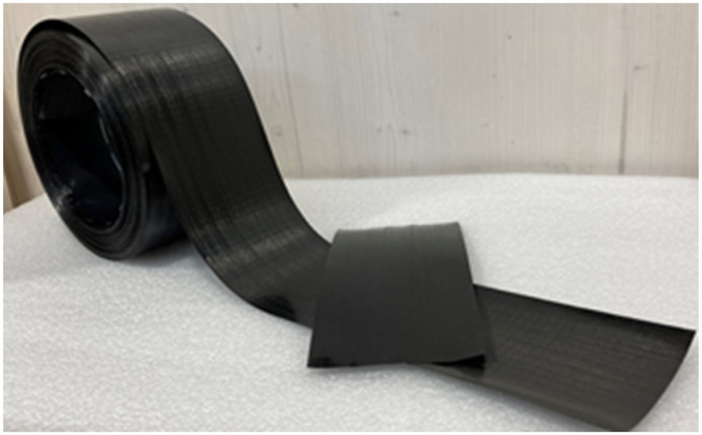

One of the production methods for UD tapes involves continuous, extrusion-based melt impregnation. Multiple fiber bundles (so-called rovings) are continuously pulled off a fiber creel and are aligned and spread next to each other to achieve a flat, unidirectional tape structure. During fiber spreading the initially compact and elliptically shaped cross-sections of the rovings are transformed into rectangular shapes. In the impregnation die, the fiber carpet is penetrated by a thermoplastic polymer melt, which is typically processed and delivered by a single- or twin-screw extruder. After impregnation, the tape is calibrated to its final shape and thickness and cooled down for final tape-winding onto bobbins.

Production defects, including gaps (empty or polymer-filled), fiber breakage, surface irregularities, and improperly impregnated fiber regions, may lead to poorer mechanical and optical tape properties. These defects are typically introduced during spreading and impregnation of the fiber tows, each of which consists of several thousand individual filaments. Many of the defects mentioned can be detected visually with a camera. In contrast, dry regions, where impregnation is insufficient, are often located inside the material and are therefore usually not visible on the surface. In the cross-sectional micrograph in Figure 2, a critical dry region in a poor-quality UD tape embedded in an orange-colored epoxy resin can be seen. Dry fiber regions have lengths of up to several meters and thicknesses in the lower micrometer up to the millimeter range. Fibers that are not embedded in the polymeric matrix are unable to transfer mechanical loads and can also act as crack initiators.

Figure 2.

Micrograph of a dry fiber region in a UD-tape cross section embedded in an orange-colored epoxy resin.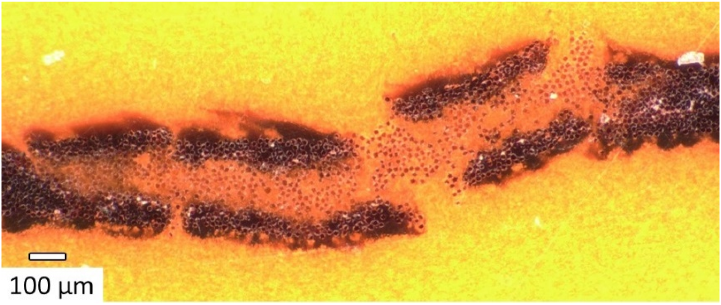

Thus, there is a need for robust quality assurance systems that use fast and non-destructive (NDT) high-resolution measurement techniques to enable efficient inline monitoring of tape quality and defects. Several measurement systems have been investigated for use in defect detection. The influence of the impregnation parameters in a melt-impregnation-based UD-tape production process on the resulting porosity and homogeneity of fiber distribution was analyzed by Hopmann et al.⁵ Duchene et al.⁶ provided a comprehensive review of various non-destructive measurement techniques for mechanical damage assessment of polymer composites, predominantly for thermosetting epoxy resins reinforced by glass or carbon fibers. Measurement methods were classified into: (i) imaging techniques, (ii) computed tomography, (iii) ultrasound, (iv) shearography, (v) infrared thermography, and (vi) terahertz spectroscopy. Banerjee et al.⁷ applied a frequency-modulated thermal-wave imaging technique to detect sub-surface defects in jute-fiber reinforced polypropylene (PP) composites.

Several experimental analyses have focused on the assessment of defects in UD composite structures. Van de Steen et al.⁸ used optical microscopy and scanning electrode microscopy (SEM) to compare various impregnation techniques in terms of the impregnation quality achieved. Barmouz et al.⁹ employed shearography as a potential defect detection method for wood–plastic composites (WPCs). Machado et al.¹⁰ used contactless high-speed eddy current probes to examine carbon-fiber reinforced unidirectional polymer ropes with several artificial defects. Defects smaller than 1 mm in length were detected successfully at an excellent signal-noise-ratio by means of a hand-held device moving at a measurement speed of 4 m/s. Several potential inline measurement systems, including active and passive thermography, confocal laser distance sensors, air-coupled ultrasonics, and eddy current analysis, were compared by Koster et al.¹¹ To evaluate tape thickness, fiber distribution, and fiber volume content of thermoplastic carbon fiber (CF) tapes, an inline measurement approach was developed by Koster et al. that combines optical thickness measurement and thermography. Essig and Kreutzbruck¹² used air-coupled ultrasonics to measure differences in impregnation quality. This method was later used by Essig and Fey et al.¹³ on a specifically designed inline test rig to detect artificially induced defects (matrix cuts, impact damage, fiber cuts, circular holes, and sharp bends) at tape speeds of up to 5.35 m/min.

Optical coherence tomography (OCT) has also been of particular interest and has been applied in various tasks involving NDT measurement of polymer composites. Only composites that are able to transmit coherent light can be investigated using OCT, while, for example, carbon fibers block incident light. OCT is a fast and contactless method for high-resolution imaging of internal structures within semi-transparent media.¹⁴ Dunkers et al.^15–18 investigated multilayer fabrics based on epoxy and vinyl-ester resins and E-glass fibers and focused on fiber-tow architecture and the detection of potential defects, such as various types of impact damage (fiber/matrix debonding, kink banding, long cracking, and matrix fracture) and voids. Awaja et al.¹⁹ studied the effects of thermal degradation on the surface of particle- and fiber-reinforced composites by using OCT. Further, OCT has been compared to some state-of-the-art measurement techniques such as confocal microscopy and X-ray computed tomography in the context of detecting impact-damaged epoxy E-glass fiber composites, where it was able to identify several types of damage: longitudinal cracking, kink banding, matrix deformation, and fiber/matrix debonding.^20,21 An ultra-high-resolution polarization-sensitive (UHR-PS) OCT technique was applied by Wiesauer et al.²² to various multi-layered GFRP specimens, and structural investigations of features as small as single fibers with diameters in the lower micrometer range were presented.

Our previous studies^23,24 demonstrated the potential of OCT as a novel and powerful NDT measurement technique for analyzing glass-fiber reinforced thermoplastic UD tapes in a series of lab-scale experiments: We developed an inline test rig that simulated the take-off movement of a tape sample in a real production line. Further, a 2D area portal system was attached that holds the OCT sensor head and thus allows transversal movement across the tape surface. Our studies confirmed the usefulness of OCT in settings where either sensor and tape are stationary or the sensor moves across a stationary tape to obtain full-cross sectional OCT scans. With this approach, dry fiber regions, edge and surface defects, and gaps (filled and unfilled) were successfully measured.

This work made our approach increasingly industrially relevant, with a tape moving past a moving sensor at a specific take-off speed. To this end, we integrated our commercial OCT system into an industrial-scale UD-tape production line located at the LIT Factory of Johannes Kepler University Linz. To achieve this, a base unit was built between the calibration and cooling units of the tape line that allows attachment of the 2D area portal and the OCT sensor. Focusing on the detection of dry fiber regions – major defects that are often internal to the material –, we first derived optimal sensor settings for inline measurement from a comprehensive design of experiments (DoE). In particular, our aim was to find an optimal balance between measurement accuracy and data size. In our experiments, prefabricated tape samples 120 mm wide were held stationary while systematically varying (i) OCT travel speed across the tape surface, (ii) A-scan sampling rates, and (iii) A-scan averaging. The optimal measurement settings thus identified were then applied to conduct experiments with moving tapes of 120 mm width at various take-off speeds of the UD-tape production line. Optical microscopy was used to determine the total defect width of the dry regions and thus assess the measurement accuracy of the OCT sensor. Finally, we developed a robust and computationally inexpensive assessment of binarized B-scan traces that computes the defect-width distribution and visualizes characteristic features as histograms or spider plots.

Fundamentals: optical coherence tomography

OCT was introduced in the 1990s and originally developed for non-invasive and non-destructive biomedical investigations in ophthalmology.²⁵ Since its introduction, OCT has been used in an increasing range of applications in material science and biomedicine.^26,27 It relies on white-light interferometry using high spatial but low temporal coherence light sources, typically in the near-infrared (NIR) range of 1-15 µm, and yields excellent axial resolutions.²⁸ OCT is well suited to use with image-layered or micro-structured samples as detection is based on interferometry, where the image contrast results from inhomogeneities in the refractive index within the sample material.²⁹ Spectral Domain (SD-) OCT uses the Fourier Domain (FD-) OCT technique, where the spectrum contains the depth information as an axial distribution (A-scan).²³

Figure 3(a) shows a schematic of an OCT system that is based on a Michelson interferometer. The low-coherence light beam exiting the light source is split into two beams, one of which is pointed directly at the sample surface. The other beam is directed to a movable reference mirror to allow depth scans.

Figure 3.

Schematic of an optical coherence tomography system based on a Michelson interferometer (a) and the two fundamental scanning routines in the X/Y-plane (b).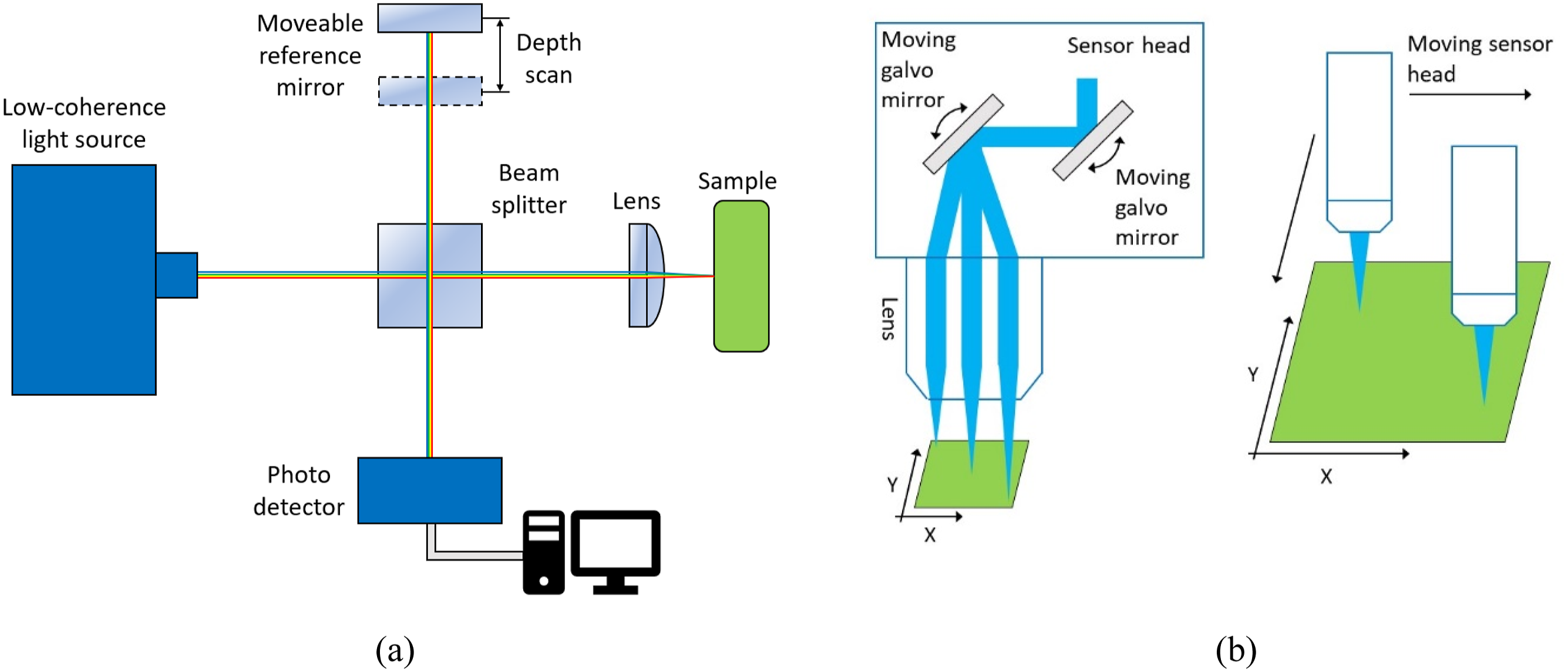

Figure 3(b) compares the two fundamental scanning routines for planar measurement. Internal galvo mirrors allow fast, precise manipulation of the measurement axis and therefore scanning of a plane but are typically limited to a maximum possible area in the lower mm² range. Another approach keeps the measurement axis fixed but moves either the OCT sensor head or the sample itself in the plane. Any arbitrary plane can be covered, but at the cost of significantly lower mapping speeds. As in acoustic investigations, one-dimensional point measurements are called A-scans. Multiple A-scans along a line lead to a two-dimensional B-scan. Multiple B-scans over an area yield a volume scan, and so-called en-face or C-scans can be created from areal scans at a defined depth position (see Figure 4). Additionally, the acquisition of consecutive A-scans at one constant lateral position can generate information about progress over time (M-scan).

Figure 4.

Data recording via A-scan (= depth profile), B-scan (= multiple A-scans along a line), volume scan (= multiple B-scans of an area), and en-face or C-scan (= area scan at a defined depth).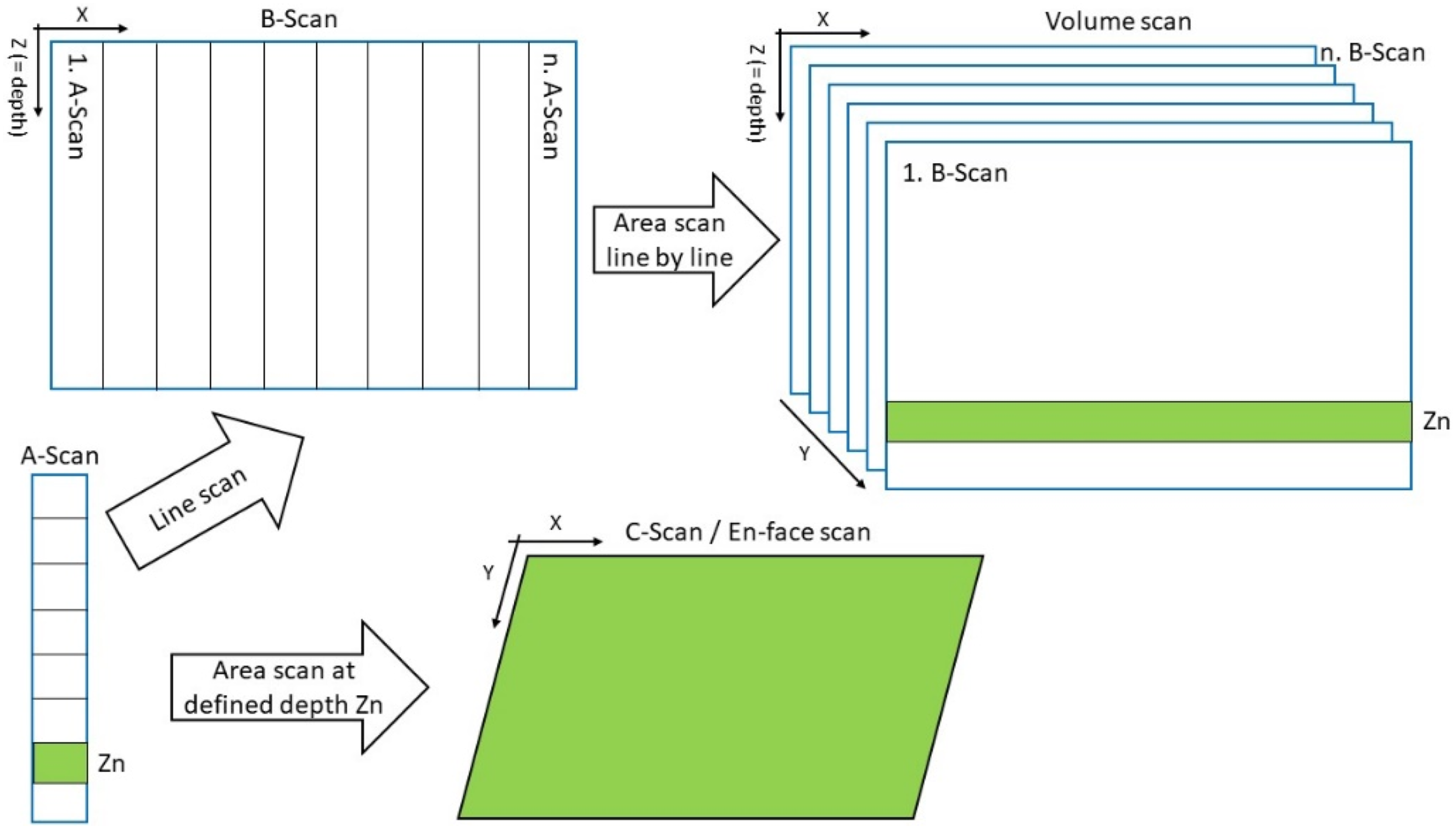

Experimental

Materials

In all experiments, prefabricated UD-tape samples consisting of a thermoplastic polycarbonate (PC) matrix and glass fibers (GF) with a fiber volume content of roughly 44% were used. The tape was 120 mm wide and 0.2 mm thick. The PC has a glass transition temperature of 145°C, a melt flow rate of 37 g/10 min (300°C/1.2 kg) and a solid density of 1192 kg/m³). The GF has a filament diameter of 17 µm, a linear density of 2400 tex (g/km), a solid density of 2620 kg/m³ and a tensile strength in the range of 2200 – 2500 MPa.

Production line for thermoplastic UD tapes

The UD-tape production line (Leistritz Extrusionstechnik GmbH, Nuernberg, Germany) used in this study is located at the LIT Factory of Johannes Kepler University Linz. Its main components are illustrated in Figure 5. The fiber creel can accommodate up to 32 bobbins. A mechanical spreading unit brings the fiber bundles together and spreads them to form a homogeneous fiber carpet. A ZSE27 co-rotating twin-screw extruder, manufactured by Leistritz Extrusionstechnik GmbH, is used to melt polymer granules and deliver the melt to the impregnation die. The impregnated fiber carpet is immediately calibrated and cooled to its final shape and thickness within the calibration and cooling units. The take-off unit generates the necessary tractive forces and speeds, and a two-stage winder in combination with a storage unit allows continuous tape production. The tape line is capable of producing UD tapes with thicknesses between 0.1 and 0.4 mm and tape widths between 100 and 300 mm at production speeds ranging from 1 to 35 m/min.

Figure 5.

Schematic of the thermoplastic UD tape production line at the LIT Factory.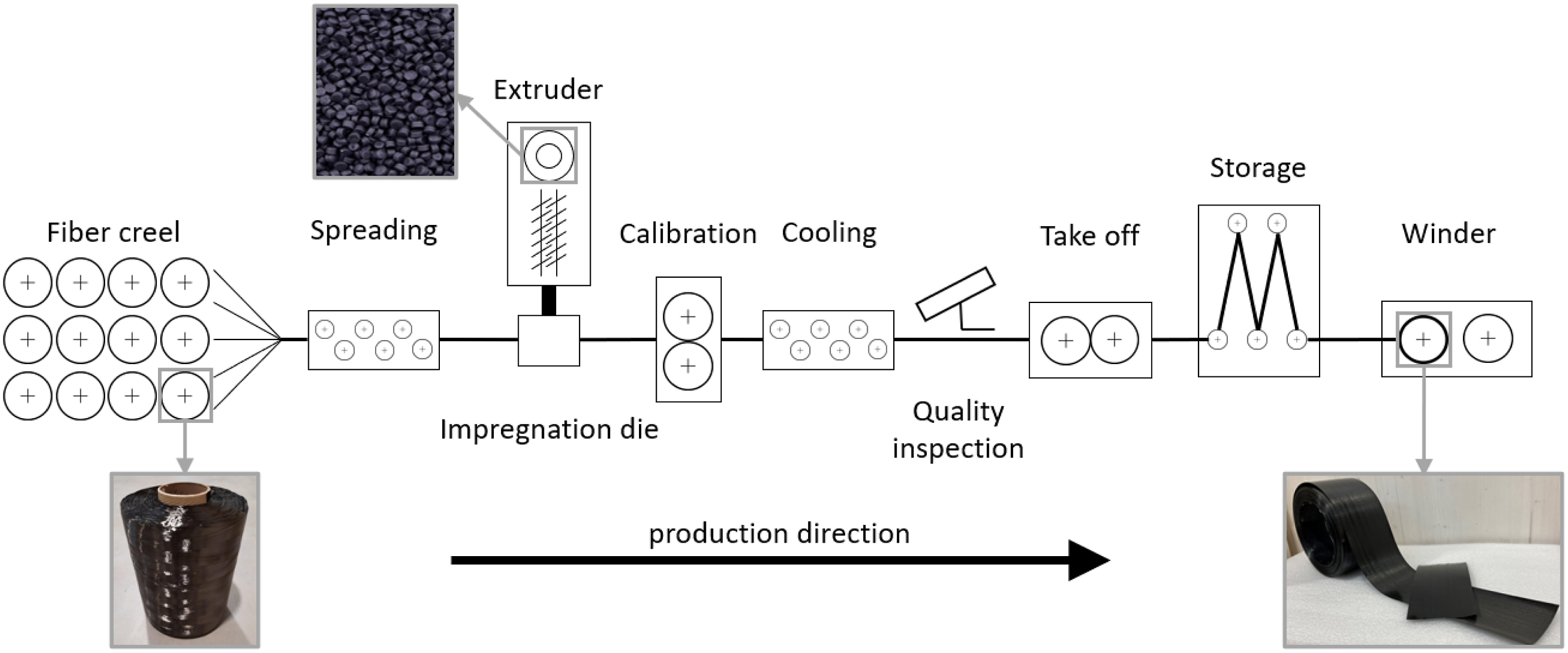

For measuring prefabricated UD-tape spools (pulled through the entire tape line), a simple wind-off module was implemented ahead of the spreading unit, as shown in Figure 6. To keep the tape in the center of the production line and restrict lateral floating of a spool, four additional guidance rings were placed on both tape edges directly at the spool site and at the first redirection roller.

Figure 6.

Wind-off module for prefabricated UD-tape spools.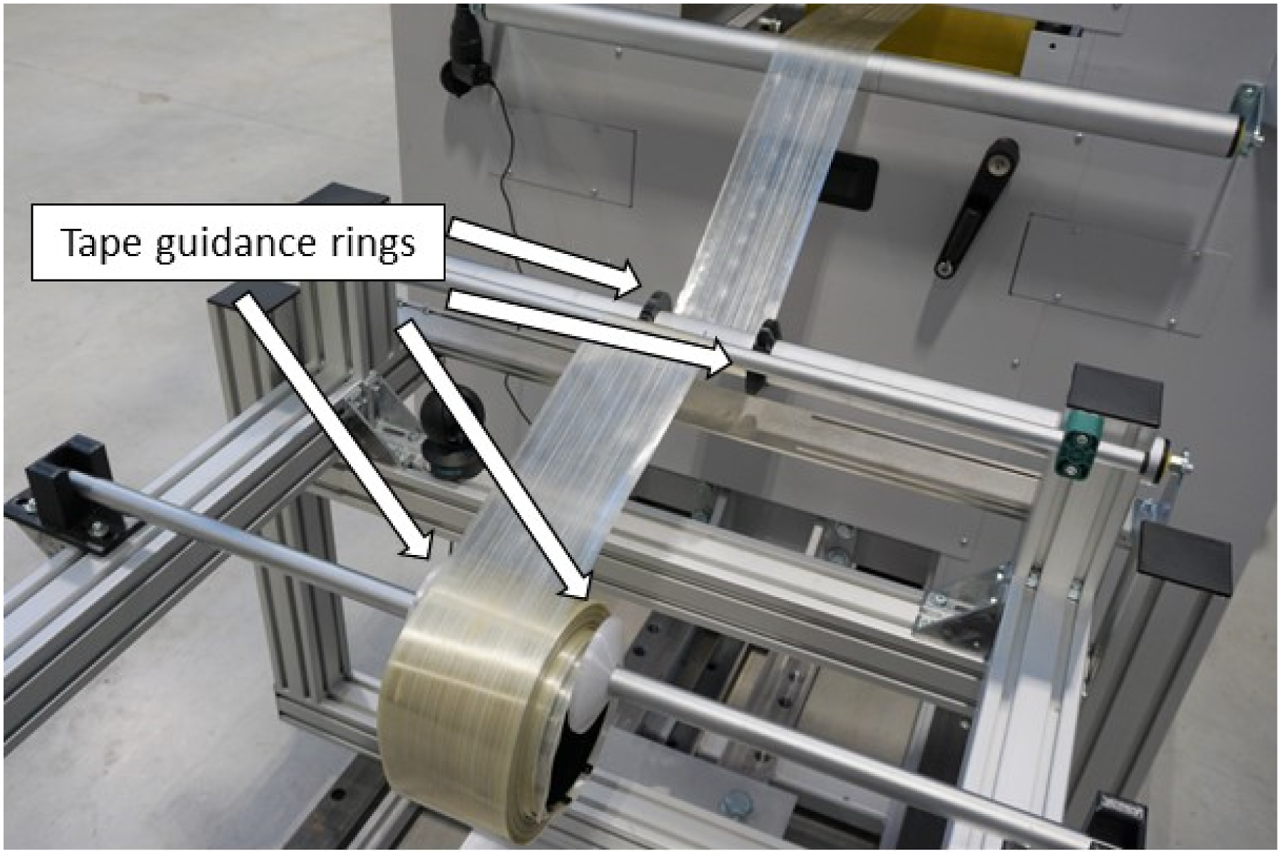

Measurement systems

SD-OCT system thorlabs TEL231

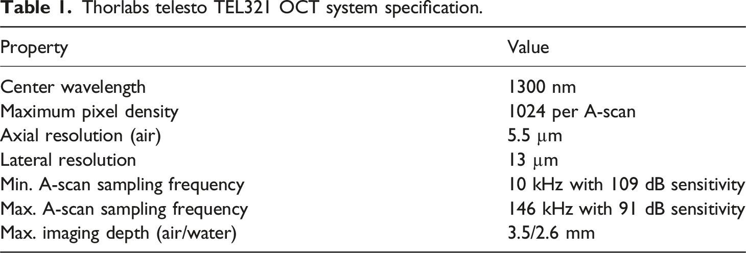
A commercial Thorlabs Telesto TEL321 OCT system in the spectral domain (SD) configuration was used that operates at a center wavelength of 1300 nm. The OCT scanner was equipped with a (Thorlabs) LK-4 lens kit, which has a maximum field of view of 16 × 16 mm² and a working distance of 41.6 mm. Table 1 summarizes the system specifications of the OCT equipment.

Table 1.

Thorlabs telesto TEL321 OCT system specification.

Property	Value
Center wavelength	1300 nm
Maximum pixel density	1024 per A-scan
Axial resolution (air)	5.5 µm
Lateral resolution	13 µm
Min. A-scan sampling frequency	10 kHz with 109 dB sensitivity
Max. A-scan sampling frequency	146 kHz with 91 dB sensitivity
Max. imaging depth (air/water)	3.5/2.6 mm

Digital microscope Keyence VHX-7000

For microscopic analysis of the UD tapes, a commercial optical Keyence VHX 7000 microscope with a dual lens kit was employed, which allows magnifications ranging from 20x to 2000x.

Optical coherence tomography measurement procedure

A base unit that allows attachment of the Thorlabs OCT sensor was built and placed between calibration unit and cooling station of the UD-tape line, as illustrated in Figure 7(a). A 2D area portal with its own control unit and supplied software rests on top of the base unit. The OCT sensor head is mounted on the Y carriage of the portal (which travels perpendicularly to the fiber/production direction) at the correct working distance between sensor and tape surface.

Figure 7.

OCT inline measurement setup and tape-line integration (a). Sequential circular flow chart of the continuous OCT measurement procedure (b).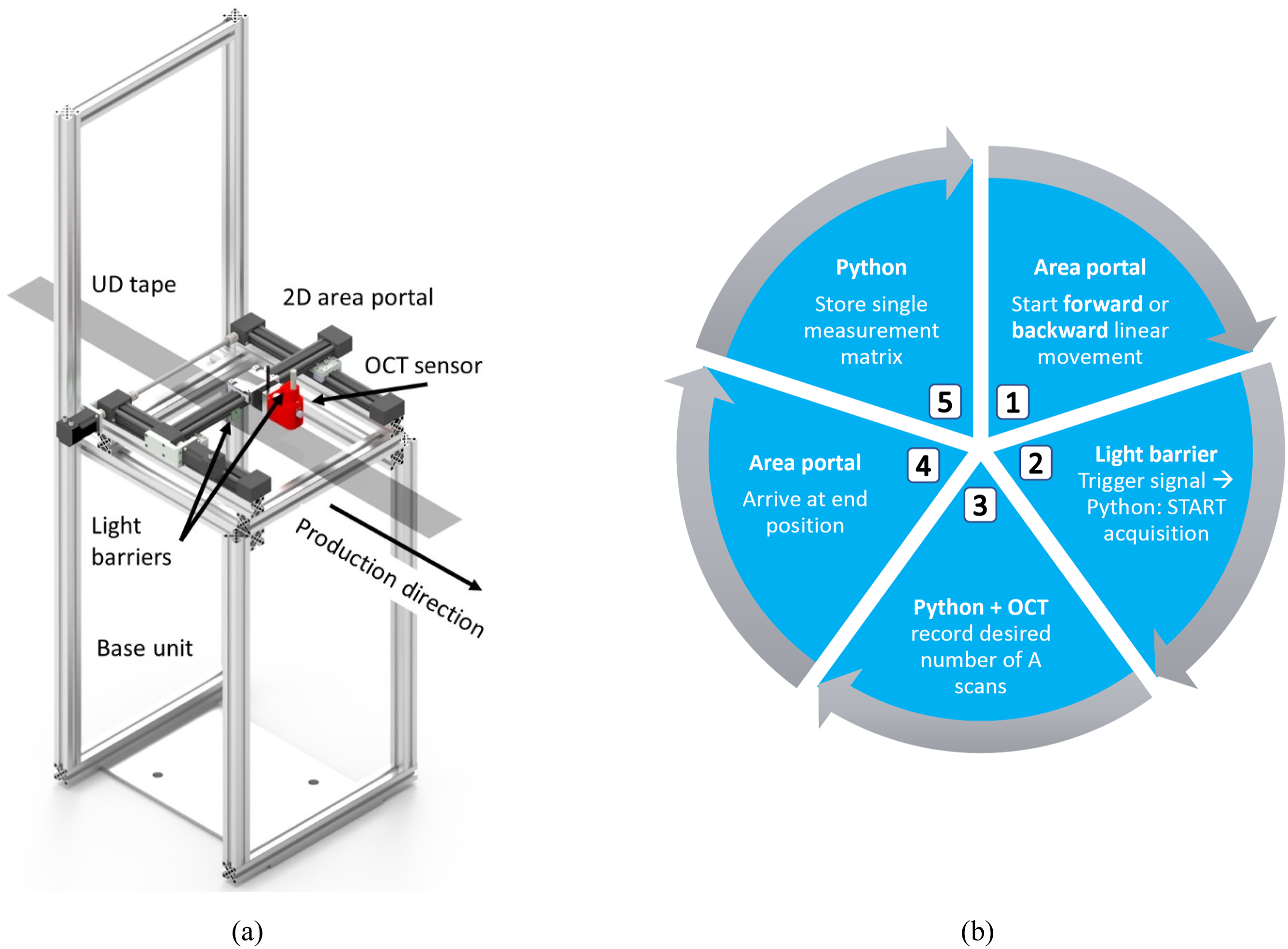

Figure 7(b) presents a sequential flow chart of the quasi-continuous OCT measurement procedure. In step (1) the carriage, with OCT sensor attached, accelerates to a selected target velocity and starts linear movement in the Y direction perpendicular to the fiber direction across the tape surface. Traveling at constant velocity, the carriage passes the first light barrier in the travel direction and thus sends a digital trigger signal (LVTTL 3.3 V) to the OCT main unit to start measurement (2). While moving at a constant velocity across the tape surface, a Python program in combination with the OCT sensor records the predefined number of A-scans needed (3). Computation of this number by $int (\frac{l_{O C T}}{v_{O C T}} f_{S})$ , where $l_{O C T}$ is the distance to be measured, $v_{O C T}$ the OCT travel speed across the tape surface, and $f_{S}$ the A-scan sampling rate, involves a rounding step. The OCT system is capable of combining and averaging multiple adjacent A-scans during measurement to minimize noise and data size while decreasing lateral resolution at the same time. In step (4), the sensor reaches its end position, and the data matrix of the currently created B-scan is stored on the hard drive in a raw data format for subsequent data evaluation (5). Any arbitrary number of measurement cycles can be performed.

The portal system has an effective maximum working area of 300 × 300 mm² and a maximum payload of 8 kg. It can travel at a maximum speed of 0.5 m/s and acceleration of 1.0 m/s².

Useful information can only be extracted from OCT scans made with a sensor moving at constant speed. Measurement acceleration or deceleration leads to stretching or compression – and thus invalidation – of the B-scan. Acceleration periods (which occur when the sensor movement changes direction) therefore limit the lateral travel speed of the OCT sensor for a predefined travel distance. For five transversal sensor velocities, the distance with constant sensor velocity (i.e., the actual OCT measurement distance) was determined, as listed in Table 2.

Table 2.

Influence of OCT travel speed on measurement distance.

$v_{O C T}$ m/s	$a_{O C T}$ m/s²	$l_{p o r t a l_\max}$ m	$t_{a c c}$ s	$l_{a c c}$ m	$l_{u n i}$ m
0.1	1.0	0.3	0.1	0.005	0.290
0.2			0.2	0.020	0.260
0.3			0.3	0.045	0.210
0.4			0.4	0.080	0.140
0.5			0.5	0.120	0.050

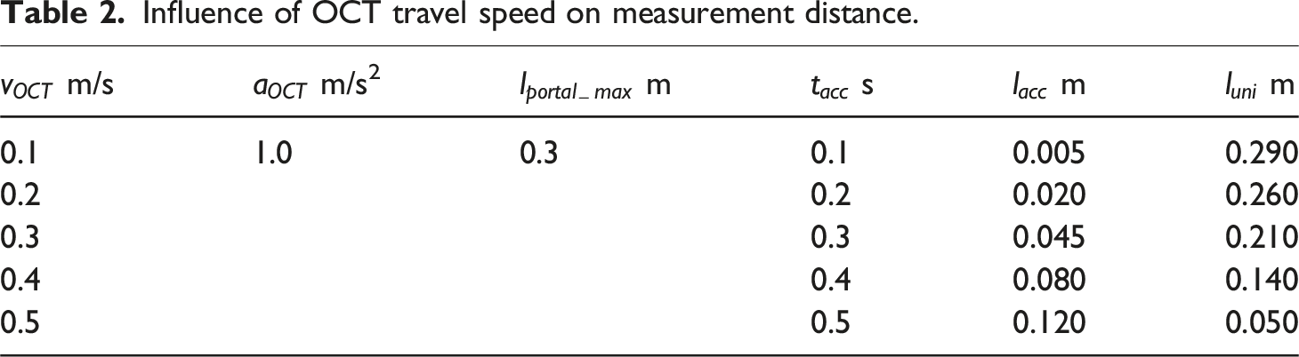
Figure 8(a) shows the velocity profile of the sensor over the travel distance for a constant acceleration/deceleration of 1 m/s² and for the two set velocities of 0.4 and 0.5 m/s.

Figure 8.

(a) Velocity profile of the 2D area portal for a constant acceleration of 1 m/s² and the two maximum velocities of 0.4 and 0.5 m/s. (b) Visualization of the resulting angle α.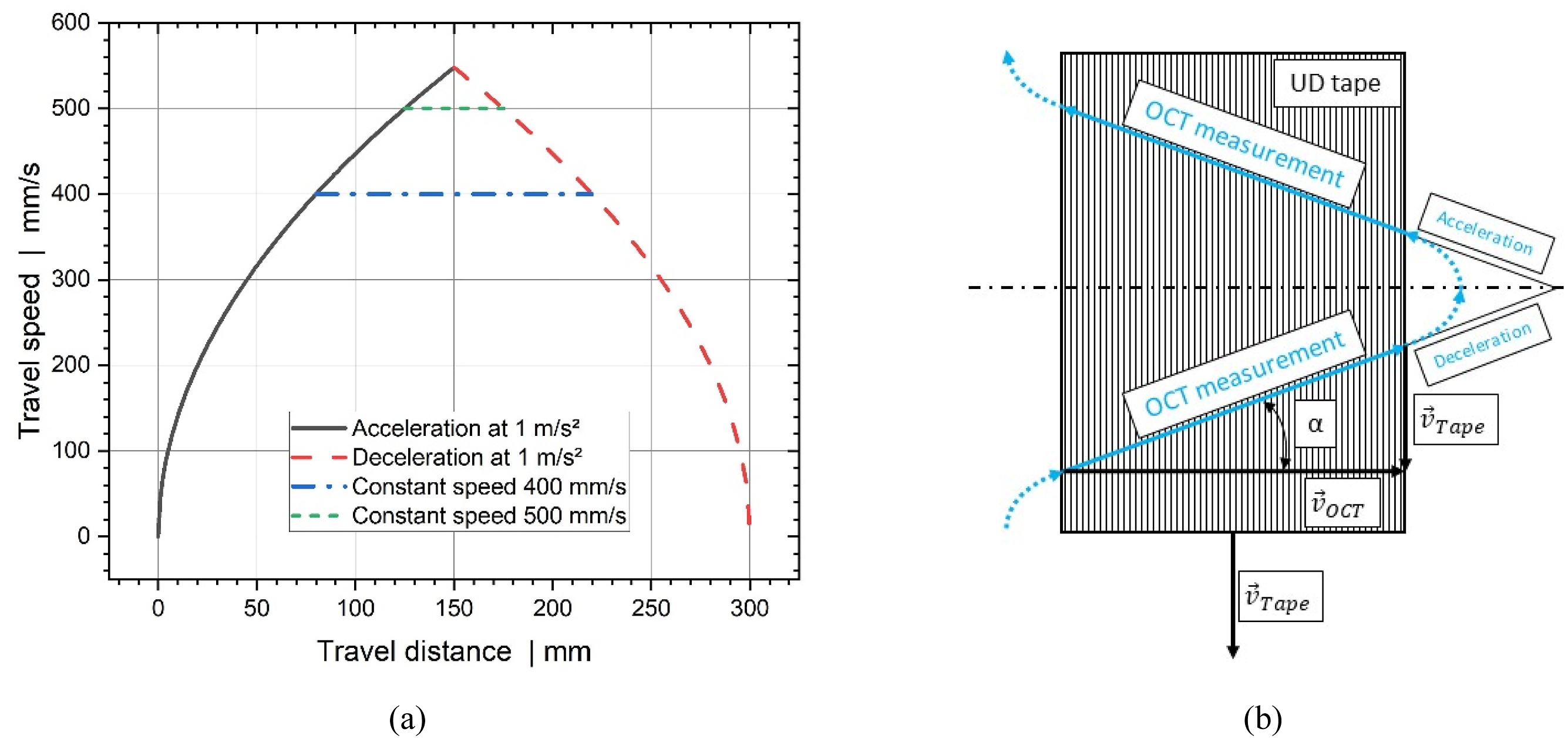

Because of the relative velocities of sensor and tape, the direction of the scan is given along an angle α by: $α = \arctan (\frac{v_{T a p e}}{v_{O C T}})$ , which is visualized in Figure 8(b). UD tapes with a maximum width of 140 mm can be investigated at a speed of 0.4 m/s (blue dash-dotted line). An increase in travel speed to 0.5 m/s reduces the maximum possible tape width to just 50 mm (green dashed line), see Figure 8(a).

Minimum defect length and lateral resolution

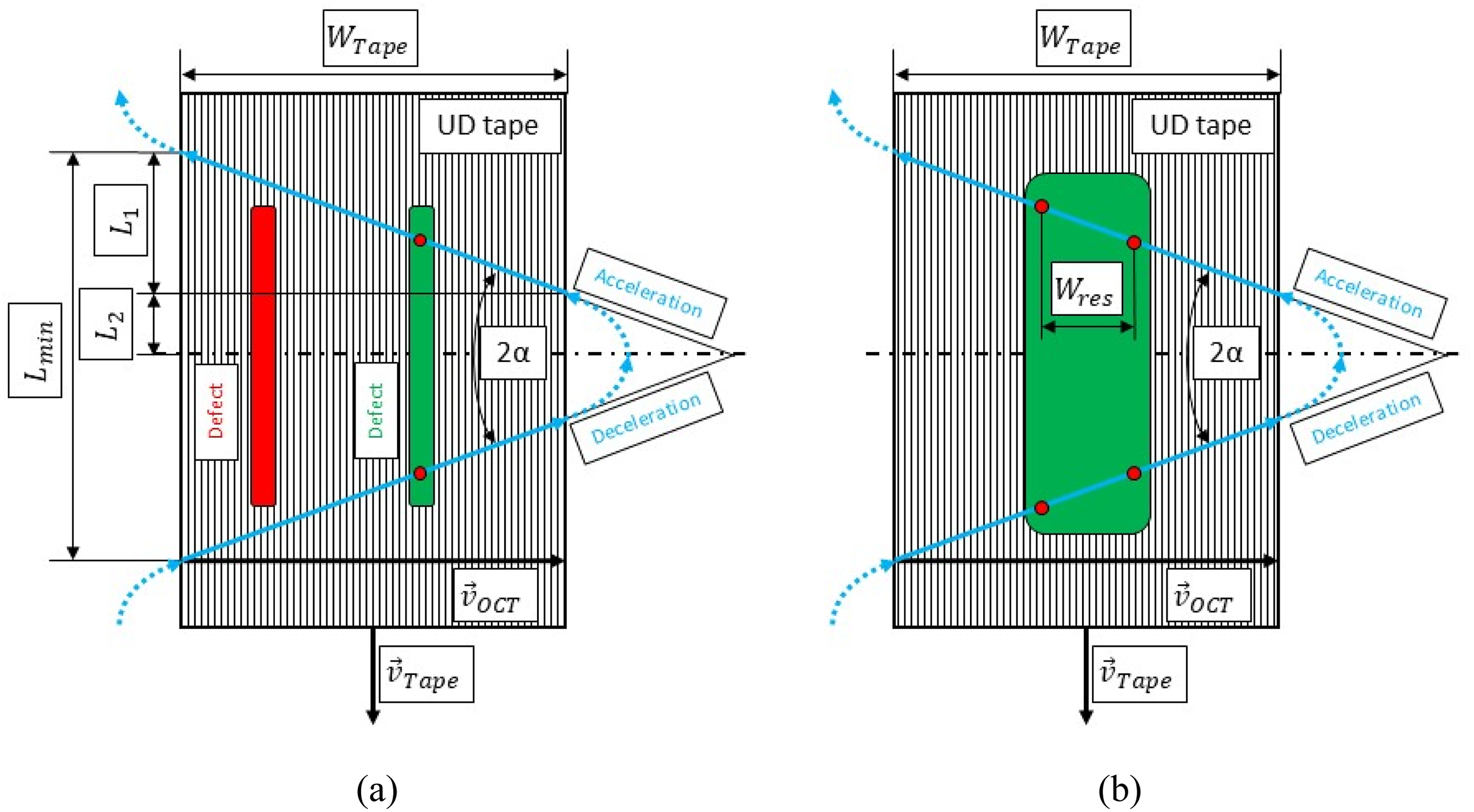
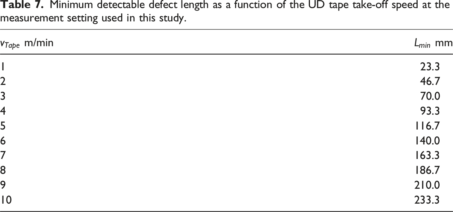
Given a specific UD-tape take-off speed, there is a minimum defect length in the tape direction $L_{\min}$ that will be detected with certainty, and it is related to the tape length scanned in two consecutive scanning cycles. It is calculated by using equation (1) and depends on the tape width $W_{T a p e}$ , the velocities $v_{T a p e}$ and $v_{O C T}$ , and the portal acceleration $a_{O C T}$ . Variables $L_{1}$ and $L_{2}$ represent the forward feeds of the UD tape while the sensor is moving at constant ( $v_{O C T} = c o n s t .)$ and non-constant ( $v_{O C T} \neq c o n s t .)$ speeds, respectively.

L_{\min} = 2 * (L_{1} + L_{2}) = 2 * (W_{T a p e} * \tan (α) + \frac{v_{T a p e} * v_{O C T}}{a_{O C T}}) .

(1)

Figure 9(a) shows that defects shorter than $L_{\min}$ may or may not be detected, depending on the lateral sensor position relative to the tape. The lateral resolution $W_{R e s}$ can be defined by the separation between two consecutive A-scans (as illustrated in Figure 9(b)). It depends on the OCT travel speed $v_{O C T}$ , A-scan averaging $a v g$ , A-scan sampling rate $f_{S}$ , and the angle $α$ :

W_{Res} = \frac{v_{O C T} * a v g}{f_{S}} * \cos (α) .

(2)

Figure 9.

(a) Minimum defect length in the fiber direction that can be detected with certainty. (b) Lateral resolution between two A-scans. The red dots indicate single A-scans on a defect outlined by a green rectangle.

Experimental tests 1: Moving sensor and stationary tape

The 2D area portal system equipped with the OCT sensor was mounted on a base unit between the calibration and cooling units of the UD-tape production line.

We used a prefabricated spool of PC/GF tape (see section Materials) that was installed into and tensioned in the UD-tape production line. To reduce tape vibrations, an additional supporting steel rod was placed immediately after the measurement position.

In UD-tape manufacturing, it is commonly assumed that tape defects with a width-to-height ratio greater than 1 are critical for industrially relevant tape qualities. This means that, for our samples with a thickness of 0.2 mm, we should be looking for defects wider than 0.2 mm. For the experiments with stationary tape, we chose a section with a 478 µm wide dry region corroborated by microscopy.

To enable accurate and quick identification of the region of interest (ROI) across the DoE experiments, the surrounding area was bounded with a self-adhesive copper tape, which strongly reflects the OCT signal. One tape edge was also marked with a copper tape to avoid ambiguity relating to the measurement direction. Figure 12(a) shows the dry ROI (recorded and measured by a digital microscope). Since the goal here was to determine optimal settings for inline measurement, we deliberately chose a fault (a dry region) with dimensions that, according to industry experience, are critical. In order to be able to determine the influence of the measurement settings on measurement accuracy and data size, all experiments were carried out with the same dry region. For all measurements, the tape was kept stationary, and the sensor settings were varied systematically, as listed in Table 3.

Table 3.

Full-factorial DoE for determining the optimal inline settings with stationary tape, where x is a number between 0 and 9.

Parameter	Unit	Min	Max	Increment	Number of levels
$f_{S}$	kHz	76	146	70	2
$a v g$	-	1	512	$2^{x}$	10
$v_{O C T}$	m/s	0.10	0.40	0.05	7

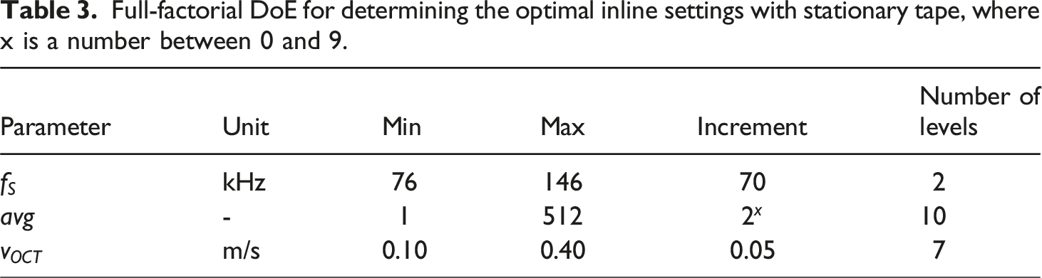
For each individual design point, five measurements were recorded, which resulted in a total of 140 design points.

Experimental Tests 2: Moving sensor and moving tape

In the next step, the previously identified optimal measurements settings were used to investigate the quality of moving UD tapes. This industrial setting produced a larger volume of more realistic data. Since our aim was to measure the quality of moving tapes, the corresponding positions of the scans needed to be tracked in a non-destructive manner to enable subsequent microscopic validation. This was complicated by the fact that the coherent light beam from the OCT is invisible to the human eye. We therefore designed and manufactured an OCT sensor housing equipped with a permanent marker at a fixed distance of $L_{S h i f t} = 48 m m$ between sensor axis and tip of the marker. Thus, we were able to correlate the OCT data with the tape region. The final sensor assembly is shown in Figure 10.

Figure 10.

The fully assembled OCT sensor including pen on the carriage of the area portal.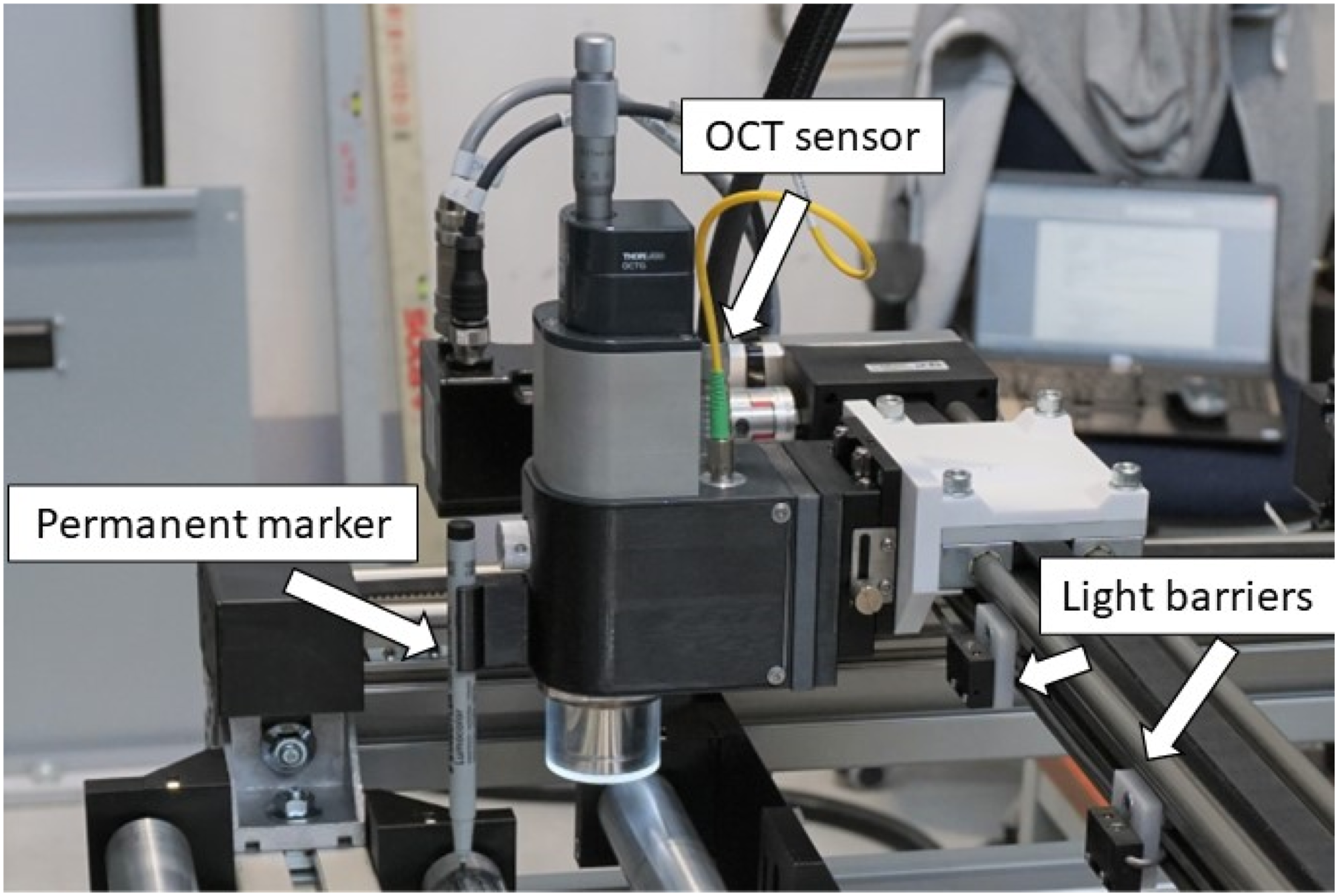

Figure 11(b) shows the basic measurement procedure for moving tapes. As discussed above, variations in the working distance can invalidate OCT measurements and should therefore be avoided. To minimize the interference and potential vibrations during movement or marking of the tape, we added three pivoted tape guidance rollers, as illustrated in Figure 11(a). Marks were made at the upper vertex of the middle roller, while OCT measurement took place immediately after the lower vertex of the first roller, where the tape detached from the roller but was still sufficiently flat. An additional flag printed by fused deposition modeling (FDM) and covered with copper tape was positioned on one side of the tape sample. Its characteristic signature in the OCT measurement allowed unambiguous assessment of the direction of measurement.

Figure 11.

Visualization of the OCT measurement paths (blue) and the leading mark lines (green) for a stationary tape (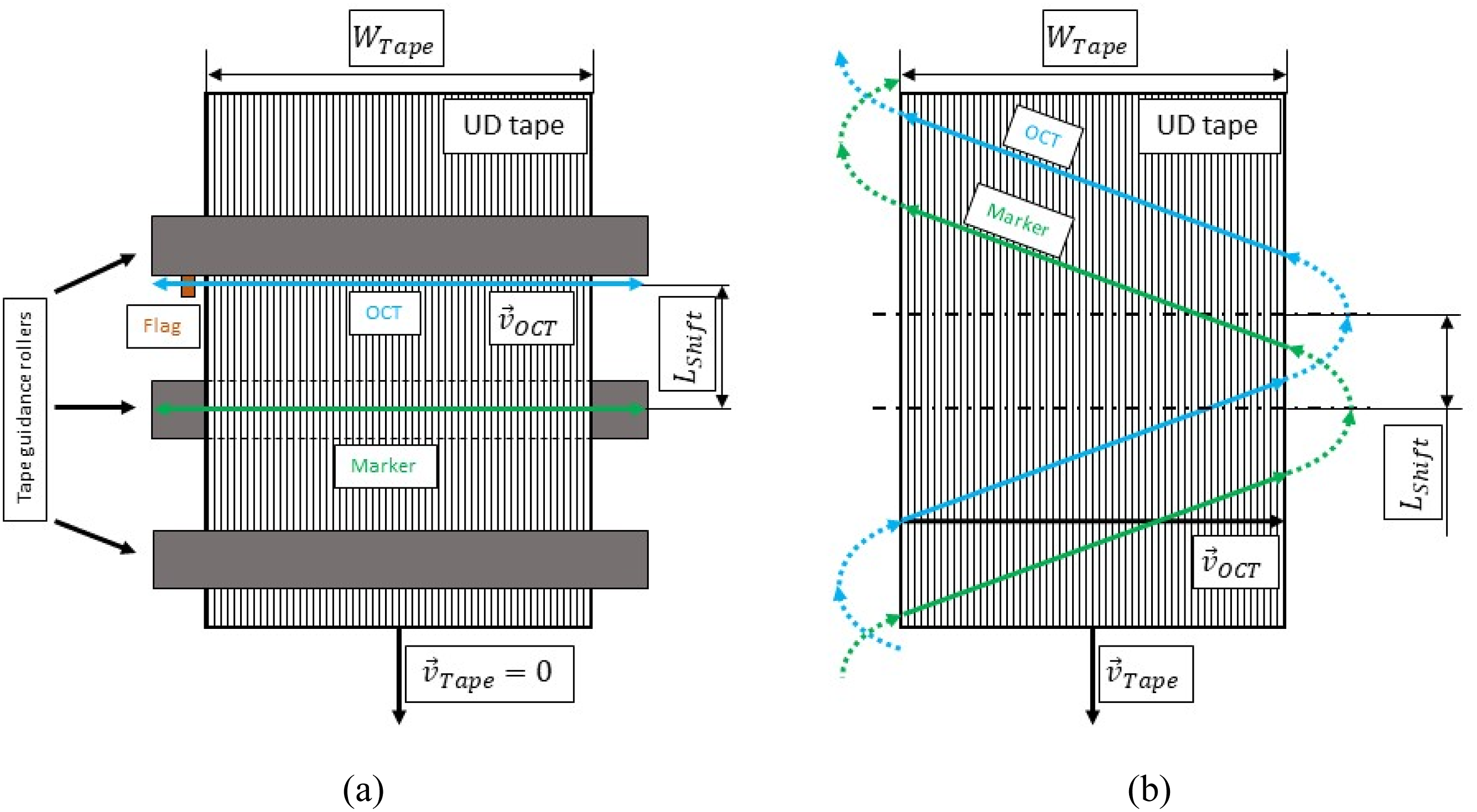 $v_{T a p e} = 0)$ at a distance of $L_{S h i f t} = 48 m m$ (a) and for a tape moving at $v_{T a p e}$ (b).

For the experimental study with moving tape samples, a sampling rate of 146 kHz and an A-scan averaging number of 8 was chosen based on our preliminary results (see Experimental Tests 1: Moving Sensor and Stationary Tape). As discussed above (see Table 2), an OCT sensor travel speed of $v_{O C T} = 0.4 m / s$ and a maximum possible acceleration of $a_{O C T} = 1 {m / s}^{2}$ allow investigation of a 120 mm wide tape sample at a constant OCT travel speed. This combination resulted in a lateral resolution $W_{Res}$ of approximately 22 µm. To take into shifts of the tape position and finite reaction times of the trigger mechanism, the overall measurement distance was increased to $l_{O C T} = 0.25 m$ . The take-off speed of the UD tape $v_{T a p e}$ was varied within an industrially relevant rage between 1 m/min and a maximum speed of 10 m/min with a step size of 2 m/min and an additional data point of 15 m/min.

To ensure that B-scans with significant defects (0.2 - 1.0 mm width) were available for evaluation of each design point, 20 B-scans were conducted for each setting.

Data evaluation procedure

Each design point was evaluated in four steps. First (1) the self-adhesive copper films were used to identify the ROI within the B-scan of the complete tape cross section, and the corresponding cropping coordinates were saved. (2) The images were then cropped manually. Steps (3) and (4), binarization and defect-width calculation, were performed in an automated manner using a Python script. Binarization led to a significant increase in contrast and thus to a clear differentiation of the defect from its surroundings. The binarization threshold critically influences the size of the defect widths observed. Here, we chose a common statistical approach frequently employed in edge detection tasks for image analysis³⁰ that is based on using the median of the grayscale image as the binarization threshold.

To evaluate the local defect width, we developed and implemented an algorithm in Python that identifies the first and the last pixel with maximum intensity (= 255 after binarization) in each row of the data matrix and calculates the distance between them, as this defines the lateral expansion of a defect. To obtain the actual defect width, the difference in pixels was multiplied by the lateral resolution $W_{Res} = 22 µ m$ . The distances were stored in a data vector that was used to determine the maximum local defect width (by a maximum-value search over all rows), as this can easily be compared to measurements taken by top-view micrographs of the tape sample. Figure 12(b) illustrates the calculation of local defect width and maximum local defect width for the ROI.

Figure 12.

(a) Micrograph of the 478 µm wide dry fiber region within the tape sample surrounded by copper tape. (b) Cropped and binarized ROI for automatic calculation of the local and maximum local defect widths.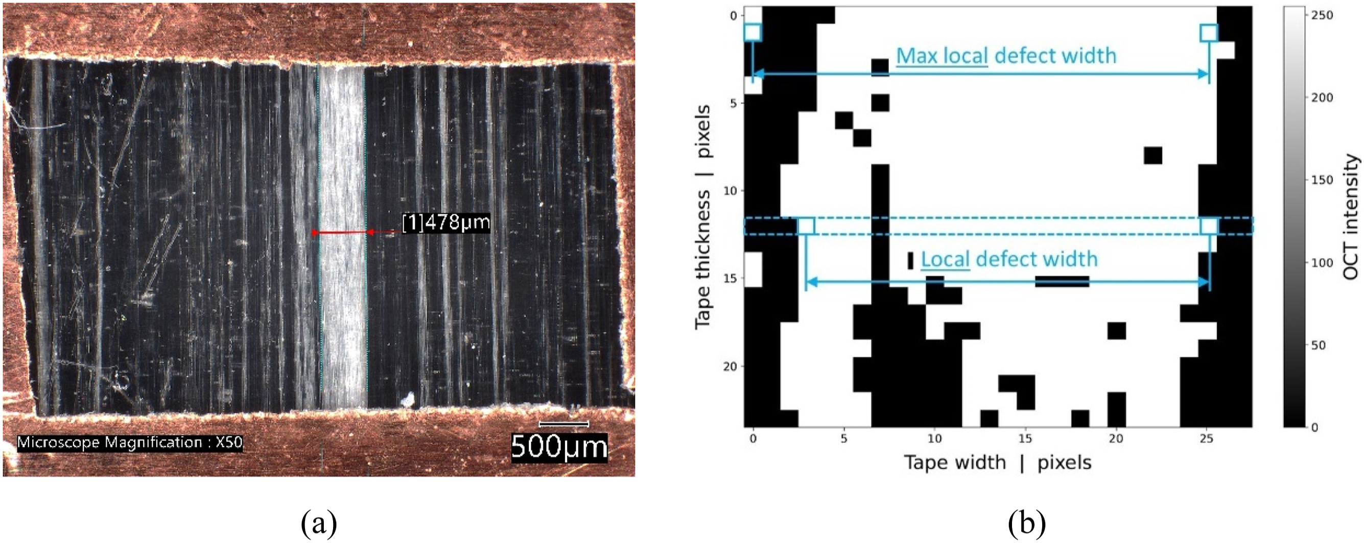

Results

Experimental tests 1: Moving sensor and stationary tape

Figures 13 and 14 display the effects of A-scan averaging, travel speed, and sampling rate on the defect size determined and on the resulting data size (see also Table 4).

Figure 13.

(a) Influence of the OCT transverse travel speed on the maximum local defect width determined for a sampling rate of 146 kHz. (b) Comparison of both sampling rates (78 kHz and 146 kHz) for the lowest and highest OCT travel speeds (0.1 and 0.4 m/s).

Figure 14.

Maximum local defect widths for OCT travel speeds of 0.1 and 0.4 m/s and corresponding data sizes.

Table 4.

Influence of A-scan averaging on lateral resolution and data size.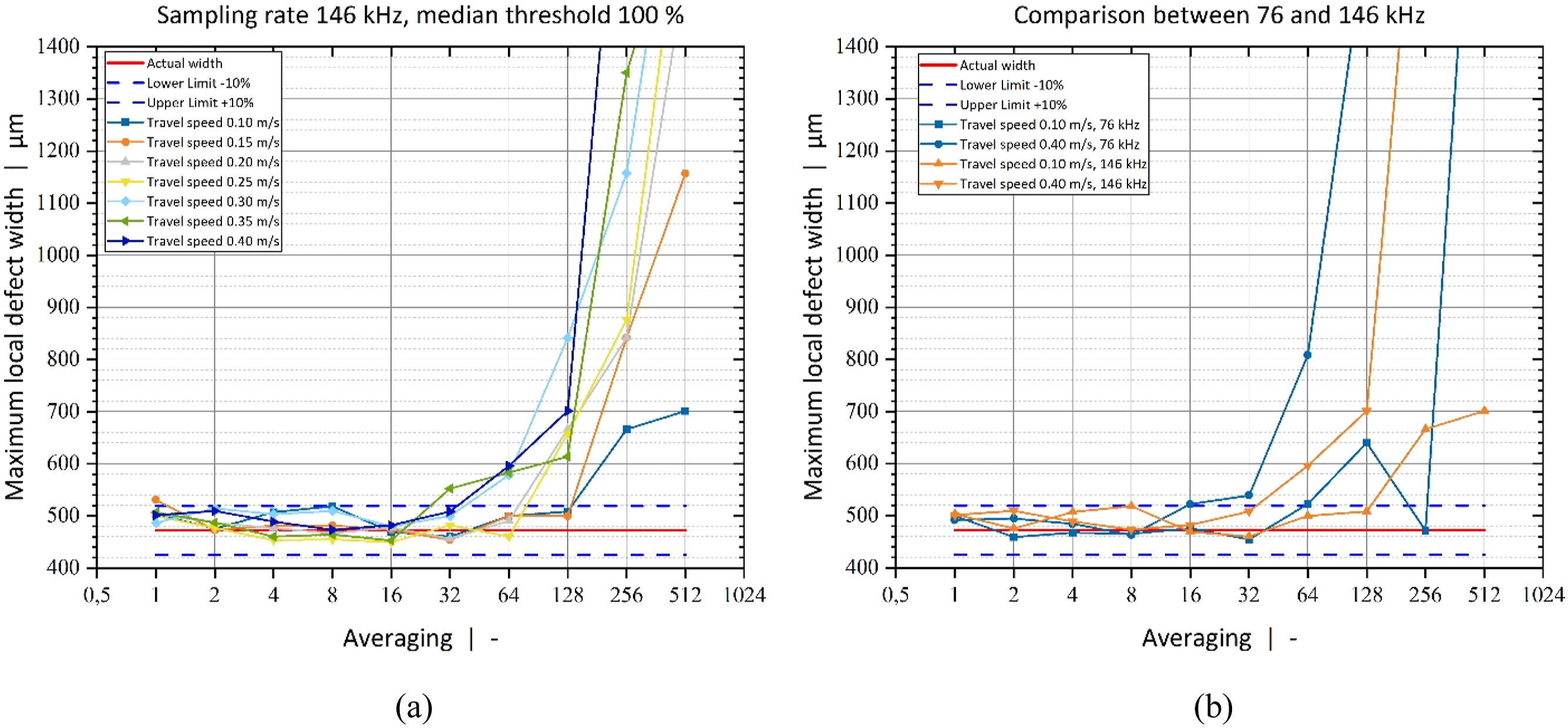

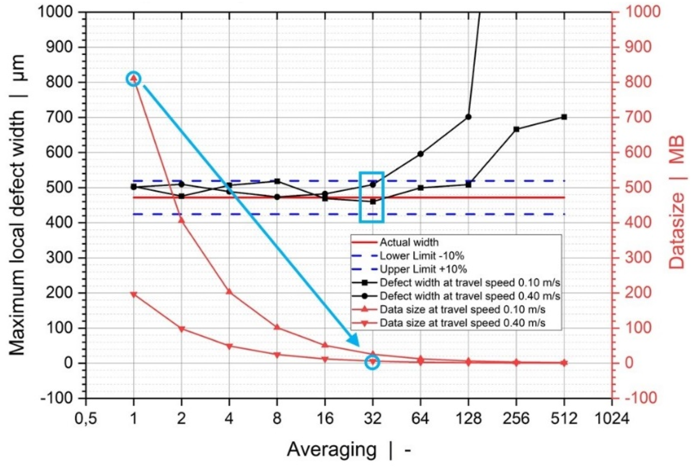
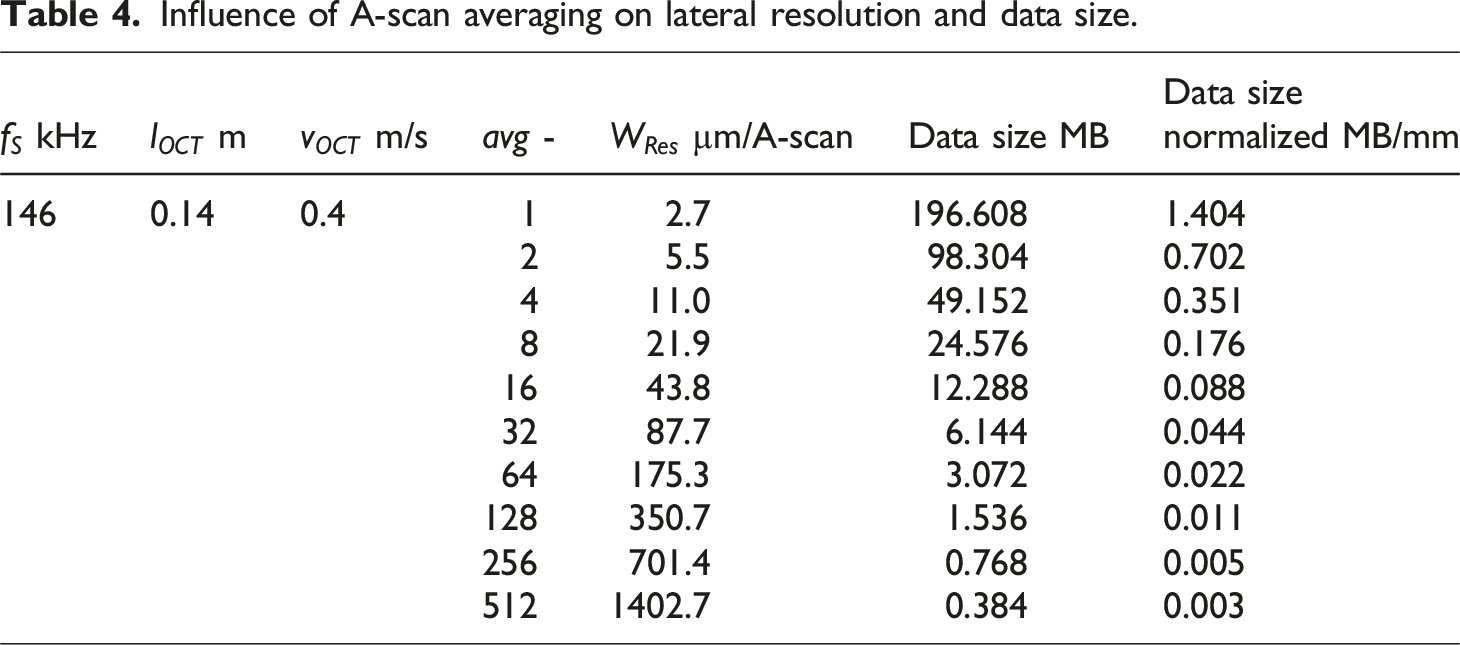
$f_{S}$ kHz	$l_{O C T}$ m	$v_{O C T}$ m/s	$a v g$ -	$W_{R e s}$ µm/A-scan	Data size MB	Data size normalized MB/mm
146	0.14	0.4	1	2.7	196.608	1.404
			2	5.5	98.304	0.702
			4	11.0	49.152	0.351
			8	21.9	24.576	0.176
			16	43.8	12.288	0.088
			32	87.7	6.144	0.044
			64	175.3	3.072	0.022
			128	350.7	1.536	0.011
			256	701.4	0.768	0.005
			512	1402.7	0.384	0.003

Figure 13 plots the maximum local defect width as a function of the A-scan averaging number. The red continuous lines in both diagrams indicate the actual defect width of 478 µm measured with the optical microscope. Two additional blue dashed lines represent an acceptable range of deviation of ±10% from the actual defect width. Figure 13(a) illustrates the influence of the OCT transverse travel speed on the maximum local defect width determined for a sampling rate of 146 kHz. The defect widths measured by OCT remained close to the value determined by the microscope up to an A-scan averaging number of around 16. A further increase caused a deviation towards higher values because the global median of the images (i.e., threshold of the binarization) decreased, which resulted in a higher probability of a pixel being classified as white. This effect was more pronounced at higher OCT travel speeds. Transverse sensor velocities showed little influence up to an A-scan averaging number of 16. Figure 13(b) compares both sampling rates (78 kHz and 146 kHz) for the lowest and highest OCT travel speeds (0.1 and 0.4 m/s). The 76 kHz measurements deviated at lower averaging numbers than the 146 kHz measurements. This is plausible because doubling the sampling rate also allows the maximum A-scan averaging number to be doubled. For an accurate assessment of defect widths using these settings, no more than 64 A-scans should be averaged.

Figure 14 shows the maximum local defect widths for 0.1 and 0.4 m/s OCT travel speed (primary/black ordinate) and the data size for each corresponding measurement (secondary/red ordinate). A potential reduction in data size is indicated for a travel speed of 0.4 m/s and A-scan averaging number of 32 (blue arrow). Data size ranged from 811 MB (0.1 m/s and no A-scan averaging) to 0.4 MB (0.4 m/s and averaging number = 512). Both the slow and the fast OCT measurements fall within the ±10% accuracy limits for maximum averaging numbers of up to 32. Traveling at a four times higher speed decreased the data size by a factor of four. Using additionally an A-scan averaging number of 32 further decreased the data size to 1/32. With 6.1 MB the resulting data size for this special case is by a factor 128 (= 4*32) smaller than the maximum data size of 811 MB. This reduction is advantageous in the context of continuous inline measurements over a longer period in terms of data traffic, storage and evaluation.

Note, however, that higher A-scan averaging numbers result in lower lateral resolutions between two consecutive A-scans. In Table 4 the influence of A-scan averaging on the lateral resolution is listed for the 146 kHz investigations. As mentioned above, for industrially relevant tape thicknesses (typically in the range of 0.2 to 0.3 mm), defects wider than 0.2 mm (i.e., aspect ratio defect width/tape thickness >1) are critical. Reliable detection of 0.2 mm wide defects requires an A-scan averaging value of 8 at a sampling rate of 146 kHz; this results in a lateral resolution of approximately ten times the absolute defect width (∼22 µm) and keeps the data size at an acceptable level of only 0.176 MB per mm measurement distance. Notably, according to the manufacturer (Thorlabs), a higher sampling rate will reduce the autocorrelation problem (i.e., slightly altered stationary copy/artifacts of the sample at the top of the image), since higher A-scan sampling rates decrease overall intensities of superimposed sample signals.³¹ This is why we favored a sampling rate of 146 kHz over 76 kHz.

Experimental Tests 2: Moving sensor and moving tape

Figure 15 shows a tape sample from the moving tape experiments with a take-off speed of 1 m/min after 12 B-scans had been recorded and marked on the surface. Note that, when identifying dry regions in OCT scans, the actual OCT scan is 48 mm behind the markings (viewed in the direction of movement).

Figure 15.

Tape sample from the moving tape experiments showing the mark lines for a take-off speed of 1 m/min.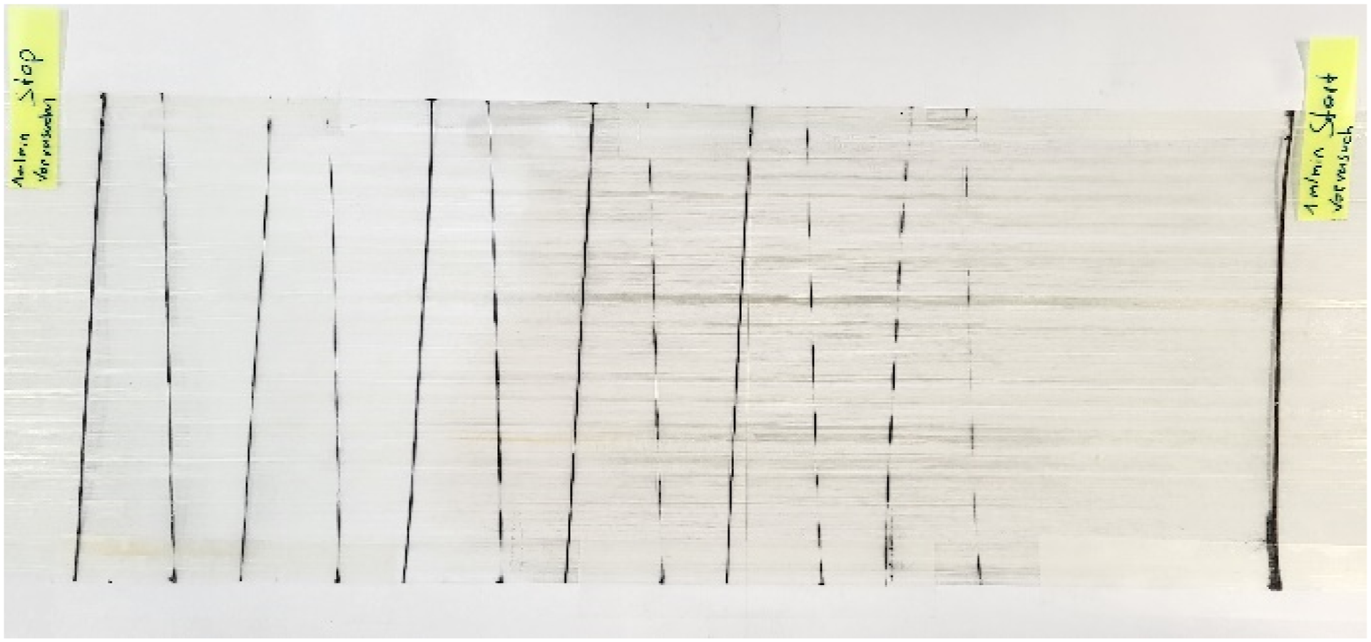

For each UD tape speed, 20 B-scans were screened manually for dry regions of widths between 200 and 1000 µm (see Figure 15). The candidates for closer inspection and their corresponding B-scan numbers are listed in Table 5. For each candidate, a blue permanent marker was used to draw a line manually that corresponded to the actual (invisible) OCT measurement line (i.e., at a distance of 48 mm parallel to the black markings from the measurement). The dry regions thus found had widths between 302 and 610 µm. The defect widths calculated using Python could be reproduced with minimum and maximum deviations of 1% and 10%, respectively.

Table 5.

Results of the experiments with moving UD tape. For all take-off speeds, actual and target angles match with minor deviations that are due also in part to manual microscope measurement.

UD tape sample	B-scan no.	Angle target	Angle actual	Defect width measured	Max. local defect width	Relative deviation
-	-	°	°	µm	µm	µm	%
MT-1	16	2.4	2.3	445	482	37	8
MT-2	18	4.8	4.9	507	504	3	1
MT-4	6	9.5	9.6	302	307	5	2
MT-6	18	14.0	14.3	390	351	39	10
MT-8	11	18.4	18.3	323	329	6	2
MT-10	15	22.6	22.7	610	548	62	10
MT-15	7	32.0	32.1	414	395	19	5

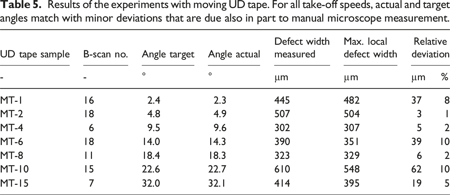
The overall performance of the OCT setup used for moving UD tapes was excellent. The targeted α angles (vector product of $v_{O C T}$ and $v_{T a p e}$ ) closely matched the actual ones, and the maximum difference between actual and calculated dry region widths was within a 10% error limit. Considering that various manual evaluation steps (microscopic measurements, B-scan cropping) and a binarization step (which significantly influences the resulting width calculation) were performed, this deviation can be deemed acceptable. Note that trigonometric calculations using the corresponding angle must be performed to achieve the final dry region width perpendicular to the fiber/production direction, as in our case only the widths in the OCT travel direction were calculated and compared.

Figures 16 and 17 present example results for take-off speeds of 2 and 8 m/min, focusing on the prominent dry fiber regions in the center of the image. In the 2 m/min take-off speed experiment (Figure 16), the dry fiber region determined had an average width of 507 µm (standard deviation STD = 15 µm). The calculated defect width resulted in a width of 503 µm and thus a deviation of only 3 µm or 1%.

Figure 16.

Results for the moving tape with 2 m/min take-off speed (MT-2). (a) Top-view micrograph showing the actual OCT measurement line in blue, and (b) cropped OCT B-scan and its binarized image (c), from which the defect widths were calculated automatically.

Figure 17.

Results for the moving tape with 8 m/min take-off speed (MT-8). (a) Top-view micrograph showing the actual OCT measurement line in blue, (b) and cropped OCT B-scan with its binarized image (c), from which the defect widths were calculated automatically.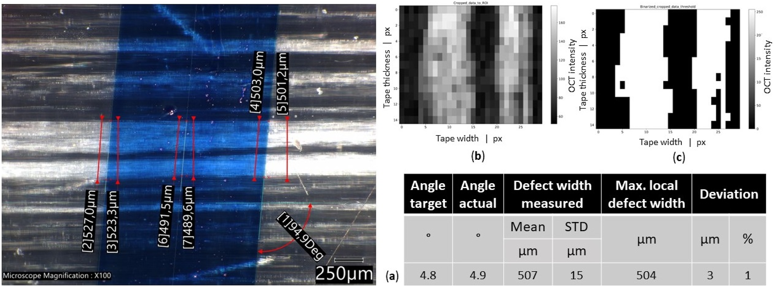

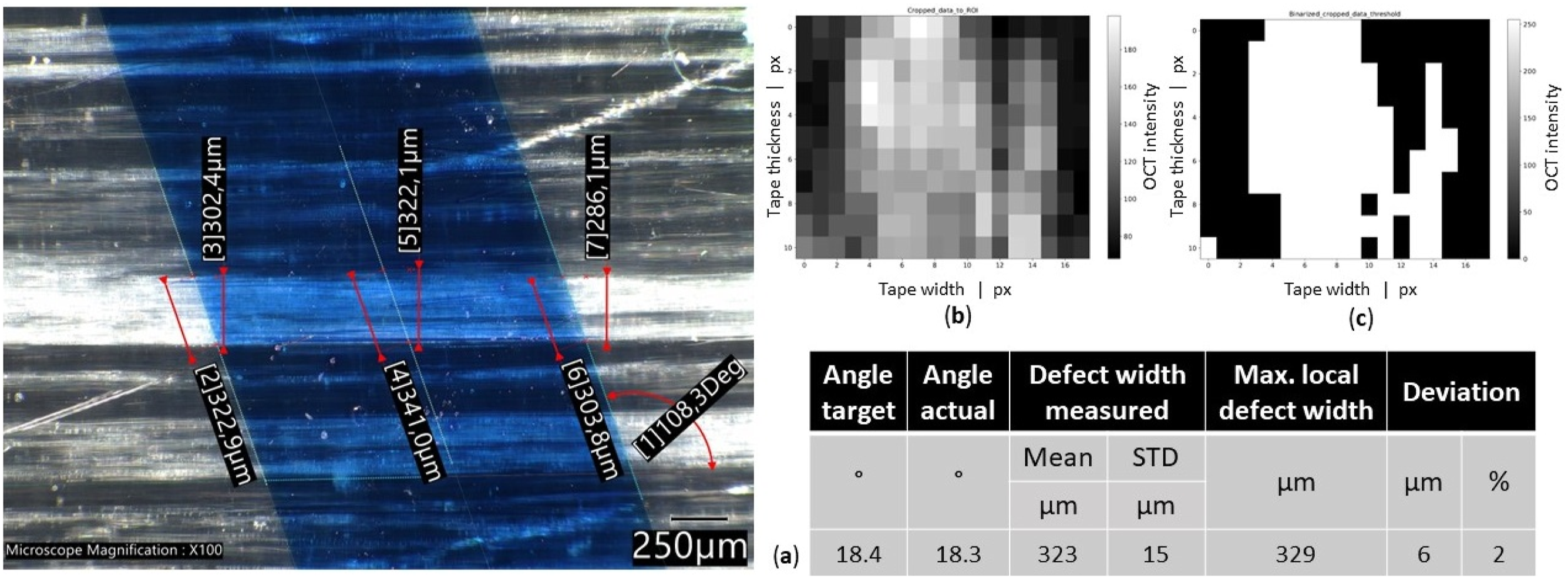
The dry fiber region in the 8 m/min take-off speed experiment (Figure 17) had an average width of 323 µm (standard deviation STD = 15 µm). The calculated defect width resulted in a width of 329 µm and thus in a deviation of only 6 µm or 2%.

A strategy for full cross-sectional quality assessment

With the aim to enable efficient real-time monitoring of dry fiber regions, we defined a workflow for the detection of dry regions across entire tape cross sections. Our approach is based on the idea of detecting ‘events’ in the tape cross section, where event refers to a sufficiently wide bright section in the OCT B-scan. To this end, (a) raw images are preprocessed (i.e., cropped and normalized because vibrations and tape wandering cause fluctuations in the working distance) to produce a straight rectangular representation of the tape cross section. The tape edges are excluded because the high OCT intensities there would interfere with the algorithm. Typical image dimensions are 5594 × 70 pixels (tape width = 120 mm, thickness = 0.2 mm). (b) To determine whether and where along its cross section the tape exhibits dry regions, the image is divided into buckets (rectangles) of 10 × 70 px, which corresponds to roughly 220 µm, that is, the critical minimum defect width assuming 0.2 mm thick tapes. For each of the buckets, the median gray value is determined and compared to the global median of gray values. For the production of the binarized (2D) image, the grayscale values are compared to a threshold. (c) For the projection onto a 1D trace (which is subsequently evaluated statistically), an aggregation step is involved that allocates 10 traces into buckets along the width of the tape. The binary trace is determined based on a comparison between the median of grayscale values in the buckets and the global median. The threshold reflects the desired detection sensitivity in a particular set of images and must be determined empirically. In the resulting traces, the value 1 corresponds to an event, that is, a local dry region. The workflow is illustrated in Figure 18, showing results for various levels of dry-region content. From the binarized trace, a histogram of defect widths can be produced, along with a histogram of defect-free regions. The left and right panels show scans with approximately 16% and 2.4% dry-region content, respectively. The histogram regions are shown for the interval [0 cm, 14 cm]. (d) The resulting trace can be conveniently described and visualized by the overall dry-region content and the distribution of defect widths. In particular, we used the mean and maximum defect sizes to quantitate the severity of the defects. This evaluation is robust, fast, and explainable, and therefore well-suited to implementation in real-time settings.

Figure 18.

Workflow for assessing dry content along a tape section.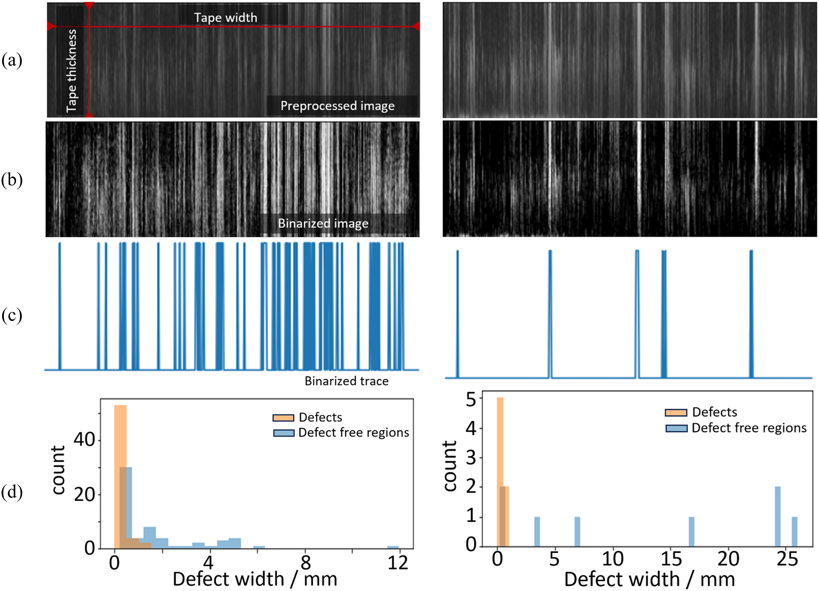

Example visualizations are given in Figure 19. The spider plot shows the overall dry content derived from the binarized trace, the maximum defect width, and the mean defect width. The red triangle represents the specimen with 16% dry-region content (corresponding to the left panel in Figure 18), and the green triangle corresponds to the specimen with 2.4% content (right panel in Figure 18).

Figure 19.

3D spider plot for visualizing dry content along a tape section.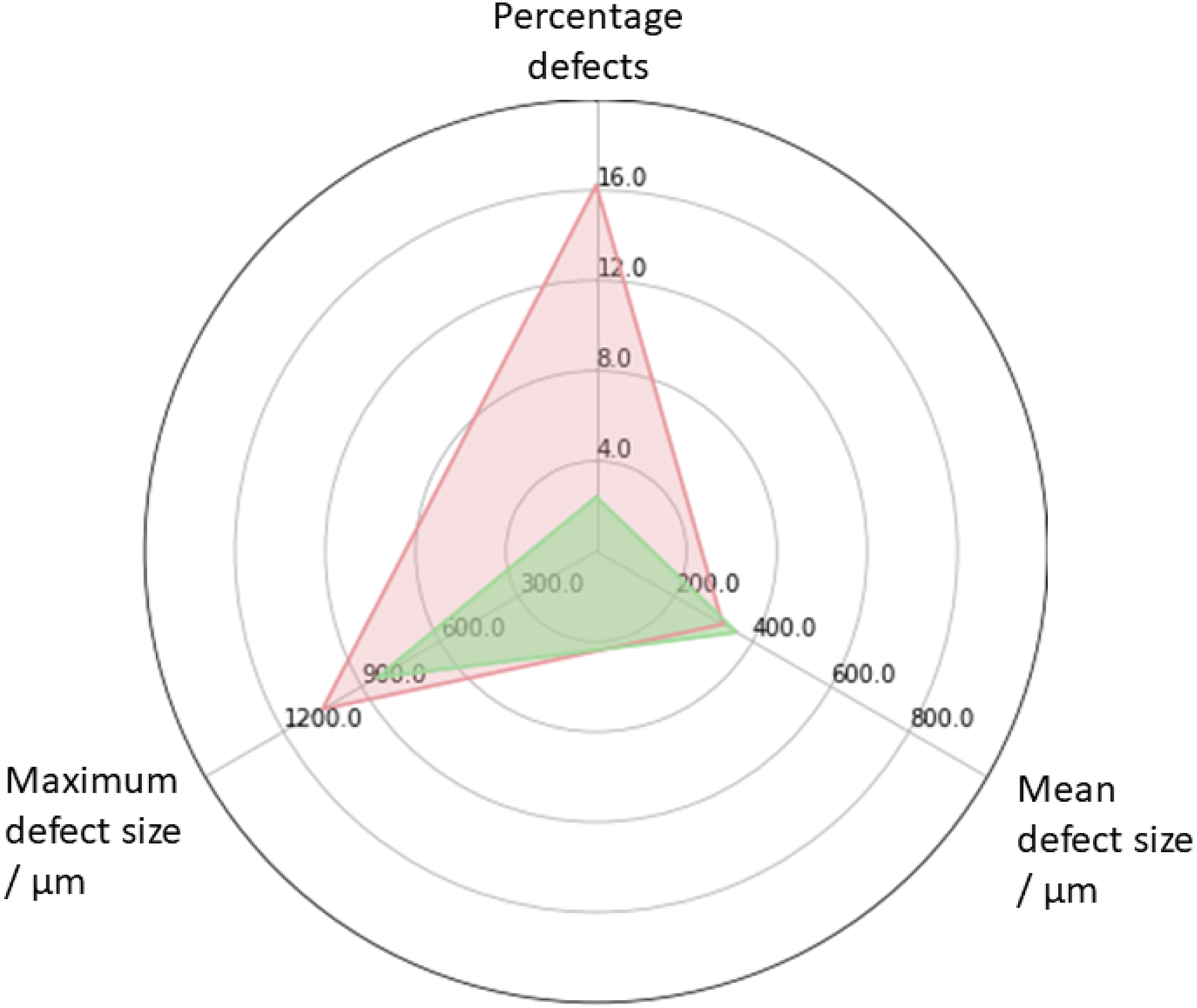

Discussion and conclusion

We successfully integrated a commercial OCT measurement system into an industrial-scale UD tape production line and conducted experiments on stationary and on moving UD tapes. We first derived optimal inline measurement parameters to achieve satisfactory accuracy at an acceptable data size. Using an OCT travel speed of 0.4 m/s, an A-scan sampling rate of 146 kHz, and an A-scan averaging number of 8, we obtained a transverse resolution of 22 µm while keeping the data size at about 0.176 MB/mm. Despite significant reduction in the amount of data there was no significant loss in accuracy. Data of this size can be stored by the computer without causing delays or interruptions in the workflow – a prerequisite for real-time data evaluation and thus for an inline monitoring scheme.

In Table 6 the optimal settings are compared to extreme settings (

v_{O C T} = 0.1 m / s

and

a v g = 1

), with a focus on the size of data collected for measurement durations of 1 h and 24 h, respectively.

Table 6.

Data size comparison between extreme and optimal inline settings.

Settings	$v_{O C T}$ m/s	$a v g$ -	Data size (1 h) TB	Data size (24 h) TB
Extreme	0.1	1	0.693	16.636
Optimal	0.4	8	0.038	0.912

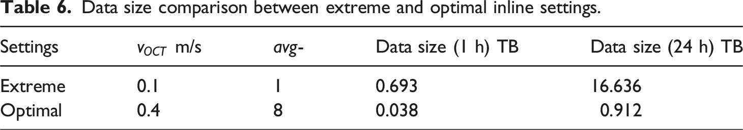
Using these optimal settings, experiments with moving tape samples were conducted within an industrially relevant range of take-off speeds between 1 and 10 m/min, and an additional maximum speed of 15 m/min. Defects with widths of 300 µm and greater were successfully identified and quantified using OCT on moving tapes. Notably, these settings allow detection of even smaller than critical defect widths (< 200 µm).

Subsequent processes, such as consolidating several tapes, can exacerbate or mitigate defects. Furthermore, the permissible tolerance thresholds are highly dependent on the final component or area of application. For example, the maximum permissible limit for dry areas is 1% by volume for the aerospace industry but 5% for other typical applications. The structure/property relationships are currently not mapped by means of standardized tests, but even the smallest irregularities in the UD tapes are sufficient to drastically reduce the mechanical properties. Levels of void content within composites are inversely correlated with fatigue life, interlaminar shear strength, and flexural strength.^32–34 An aspect ratio of maximum defect width to tape thickness of 1 has therefore been established for industrial production processes. It has been shown that modern OCT systems can successfully resolve defect widths in this order of magnitude still having reserves for the detection in the lower micrometer range.

Table 7 lists the minimum length of a defect for the OCT sensor to capture it at least once for various tape take-off speeds and using our optimized measurement settings (120 mm tape width, 0.4 m/s OCT travel speed, 1 m/s² OCT acceleration).

Table 7.

Minimum detectable defect length as a function of the UD tape take-off speed at the measurement setting used in this study.

$v_{T a p e}$ m/min	$L_{\min}$ mm
1	23.3
2	46.7
3	70.0
4	93.3
5	116.7
6	140.0
7	163.3
8	186.7
9	210.0
10	233.3

Similar transverse resolutions and data sizes can be achieved by balancing averaging and the scanning speed. For instance, to achieve a resolution of 22 µm at a sampling rate of 146 kHz, a speed of 0.8 m/s (at an A-scan averaging number of 4) or a speed of 1.6 m/s (at an averaging number of 2) could be used. Note, however, that with little or no averaging, the decrease in signal-to-noise ratio will eventually be too small for robust defect detection.

Using a binarization procedure allows the following parameters to be derived from full cross sections: (a) the overall extent of the defects compared to the tape width, (b) the mean defect width, and (c) the maximum detected defect width. These can be conveniently visualized, for instance, by histograms or spider plots. The procedure reports the quantitative descriptors of the defect-width distribution; further, it is fast, robust, intuitive, interpretable and suitable for application in a real-time setting.

Currently, the workflow is not fully automated. This is due to instabilities in tape guidance, which give rise to wandering and fluctuations in the tape and which impede automated identification of the region of interest. The relevant B-scans must therefore be identified and cropped manually. Optimization of this step, in the sense that the tape always appears in the exact same lateral position and at the same distance with respect to the sensor, would enable complete automation of the workflow (data acquisition and analysis) and automated monitoring of the production line.

The method could also be optimized by increasing the OCT travel speed, which could be achieved by using a faster 2D area portal and/or a lighter OCT sensor. This would result in a smaller angle α and a reduction in information loss between two consecutive measurements. Shorter defects in the production direction would therefore become detectable. In addition, higher OCT travel speeds would allow wider tapes to be measured with comparable minimum defect lengths.

The full cross-sectional analysis is sensitive to the binarization threshold. Generally, we expect that an inline system would have to be calibrated for different systems or environments (because, for instance, different materials, and light settings are used).

Footnotes

Acknowledgements

The authors acknowledge financial support from the COMET Center CHASE, funded within the COMET − Competence Centers for Excellent Technologies program by the BMK, the BMDW and the Federal Provinces of Upper Austria and Vienna. The COMET program is managed by the Austrian Research Promotion Agency (FFG).

Declaration of conflicting interests

The author(s) declared no potential conflicts of interest with respect to the research, authorship, and/or publication of this article.

Funding

The author(s) disclosed receipt of the following financial support for the research, authorship, and/or publication of this article: This work was supported by the Österreichische Forschungsförderungsgesellschaft; 868615.

ORCID iDs

Michael Wenninger

Christian Marschik

References

European Comission . A European green deal - striving to be the first climate-neutral continent, https://commission.europa.eu/strategy-and-policy/priorities-2019-2024/european-green-deal_en (2023, accessed 2023).

Witten

Mahtes

. Der europäische Markt für Faserverstärkte Kunststoffe/Composites 2022 2023, https://www.avk-tv.de/files/20230425_avk_marktbericht_2023.pdf

Ehrenstein

. Faserverbund-kunststoffe: werkstoffe - verarbeitung - eigenschaften. 2. Völlig überarbeitete auflage. München, Germany: Hanser, 2006.

Neitzel

Mitschang

(eds) Handbuch verbundwerkstoffe: Werkstoffe, Verarbeitung, Anwendung. 2. In: aktualisierte und erweiterte Auflage. München, Germany: Hanser, 2014.

Hopmann

Wilms

Beste

et al. Investigation of the influence of melt-impregnation parameters on the morphology of thermoplastic UD-tapes and a method for quantifying the same. J Thermoplast Compos Mater 2021; 34: 1299–1312.

Duchene

Chaki

Ayadi

et al. A review of non-destructive techniques used for mechanical damage assessment in polymer composites. J Mater Sci 2018; 53: 7915–7938.

Banerjee

Chattopadhyay

Chatterjee

et al. Non-destructive testing of jute–polypropylene composite using frequency-modulated thermal wave imaging. J Thermoplast Compos Mater 2015; 28: 548–557.

van de Steene

Verstockt

Degrieck

et al. An evaluation of three different techniques for melt impregnation of glass fiber bundles with polyamide 12. Polym Eng Sci 2018; 58: 601–608.

Barmouz

Behravesh

Reshadi

et al. Assessment of defect detection in wood–plastic composites via shearography method. J Thermoplast Compos Mater 2016; 29: 28–36.

10.

Machado

Antin

Rosado

et al. Contactless high-speed eddy current inspection of unidirectional carbon fiber reinforced polymer. Compos B Eng 2019; 168: 226–235.

11.

Koster

Summa

Jungmann

et al. Inlinetauglichkeit von zerstörungsfreien Prüfmethoden für den digitalen Zwilling von thermoplastischen Carbonfaser-Tapes, Online, 2021. DGZfP-Jahrestagung.

12.

Essig

Kreutzbruck

. Investigation of the impregnation quality of thermoplastic tapes using air-coupled ultrasound. In: Fracture and damage mechanics: theory, simulation and experiment, Mallorca, Spain: AIP Publishing, 2020, pp. 15–17.

13.

Essig

Fey

Meiler

et al. Non-contact inline monitoring of thermoplastic CFRP tape quality using air-coupled ultrasound. Atlanta, Georgia: AIP Conference Proceedings, 2016.

14.

Huang

Swanson

Lin

et al. Optical coherence tomography. Science 1991; 254: 1178–1181.

15.

Dunkers

Everett

Sanders

et al.

Imaging of composite defects and damage using optical coherence tomography advancing with composites

Proceedings of PLAST, Advancing with Composites 2000, Milan, Dates May 9-11, 2000: PLAST 2000.

16.

Dunkers

Parnas

Zimba

et al. Optical coherence tomography of glass reinforced polymer composites. Compos Appl Sci Manuf 1998; 30: 139–145.

17.

Dunkers

Phelan

Sanders

et al. The application of optical coherence tomography to problems in polymer matrix composites. Opt Laser Eng 2000; 35: 135–147.

18.

Dunkers

Phelan

Zimba

et al. The prediction of permeability for an epoxy/E-glass composite using optical coherence tomographic images. Polym Compos 2001; 22: 803–814.

19.

Awaja

Arhatari

Wiesauer

et al. An investigation of the accelerated thermal degradation of different epoxy resin composites using X-ray microcomputed tomography and optical coherence tomography. Polym Degrad Stabil 2009; 94: 1814–1824.

20.

Dunkers

Sanders

Hunston

et al. Comparison of optical coherence tomography, x-ray computed tomography, and confocal microscopy results from an impact damaged epoxy/e-glass composite. J Adhes 2002; 78: 129–154.

21.

Stifter

Wiesauer

Wurm

et al. Investigation of polymer and polymer/fibre composite materials with optical coherence tomography. Meas Sci Technol 2008; 19: 074011.

22.

Wiesauer

Pircher

Götzinger

et al. Investigation of glass–fibre reinforced polymers by polarisation-sensitive, ultra-high resolution optical coherence tomography: internal structures, defects and stress. Compos Sci Technol 2007; 67: 3051–3058.

23.

Wenninger

Marschik

Felbermayer

et al. A novel measurement approach based on optical coherence tomography for inline quality assessment of thermoplastic glass-fiber reinforced unidirectional tapes. J Thermoplast Compos Mater; 36 2022: 3943–3965.

24.

Wenninger

Marschik

Felbermayer

et al. Optical coherence tomography - a New method for evaluating the quality of thermoplastic glass-fiber-reinforced unidirectional Tapes. In: Conference proceedings of the 37th international conference of the polymer processing society, Fukuoka, Japan, 11–15 April 2022. AIP Publishing.

25.

Srivastava

Anna

Sudan

et al. Tomographic and volumetric reconstruction of composite materials using full-field swept-source optical coherence tomography. Meas Sci Technol 2012; 23: 55203.

26.

Fercher

Hitzenberger

Drexler

et al. In vivo optical coherence tomography. Am J Ophthalmol 1993; 116: 113–114.

27.

Stifter

. Beyond biomedicine: a review of alternative applications and developments for optical coherence tomography. Appl Phys B 2007; 88: 337–357.

28.

Drexler

Morgner

Kärntner

et al. In vivo ultrahigh-resolution optical coherence tomography. Opt Lett 1999; 24: 1221.

29.

Nemeth

Hannesschlager

Leiss

et al. Optical coherence tomography – applications in non- destructive testing and evaluation. In: Kawasaki

(ed). Optical coherence tomography. London, UK: InTech, 2013.

30.

Rosebrock

. Zero-parameter, automatic Canny edge detection with Python and OpenCV. https://pyimagesearch.com/2015/04/06/zero-parameter-automatic-canny-edge-detection-with-python-and-opencv/ (2015, accessed 2023).

31.

Thorlabs . How to capture the perfect OCT image 2021, https://www.youtube.com/watch?v=GngHREr-hPU accessed 30 May 2023.

32.

Almeida

SFMde

Neto

Zdos SN

. Effect of void content on the strength of composite laminates. Compos Struct 1994; 28: 139–148, https://www.sciencedirect.com/science/article/pii/0263822394900442

33.

Bowles

Frimpong

. Void effects on the interlaminar shear strength of unidirectional graphite-fiber-reinforced composites. J Compos Mater 1992; 26: 1487–1509.

34.

Saenz-Castillo

Martín

Calvo

et al. Effect of processing parameters and void content on mechanical properties and NDI of thermoplastic composites. Compos Appl Sci Manuf 2019; 121: 308–320, https://www.sciencedirect.com/science/article/pii/S1359835X19301150

Applying optical coherence tomography to inline quality monitoring of unidirectional glass-fiber-reinforced thermoplastic tapes

Abstract

Keywords

Introduction

Fundamentals: optical coherence tomography

Experimental

Materials

Production line for thermoplastic UD tapes

Measurement systems

SD-OCT system thorlabs TEL231

Digital microscope Keyence VHX-7000

Optical coherence tomography measurement procedure

Minimum defect length and lateral resolution

Experimental tests 1: Moving sensor and stationary tape

Experimental Tests 2: Moving sensor and moving tape

Data evaluation procedure

Results

Experimental tests 1: Moving sensor and stationary tape

Experimental Tests 2: Moving sensor and moving tape

A strategy for full cross-sectional quality assessment

Discussion and conclusion

Footnotes

Acknowledgements

Declaration of conflicting interests

Funding

ORCID iDs

References