Characterisation of a metal mesh heating element for closed-loop resistance welding of thermoplastic composites

Abstract

Resistance welding is one of the most suitable and mature welding techniques for thermoplastic composites. It uses the heat generated at the welding interface when electric current flows through a resistive element, mostly a metal mesh. Closed-loop resistance welding relies on indirect temperature feedback from the weld line for process control. Its implementation is more complex than the most common open-loop welding, but on the contrary, it does not, in principle, require the definition of processing windows for each welding configuration and it allows for constant-temperature welding. The temperature at the welding interface can be indirectly monitored through the resistance of the heating element. The relationship between resistance and temperature, expected to be approximately linear for a metal mesh heating element, can then be used to translate the welding temperature into a target resistance value for the process-control routine. Despite the apparent straightforwardness of this procedure, the research results presented in this article prove that different types of characterization tests yield different resistance versus temperature relations for a metal mesh heating element, which can lead to significant temperature deviations when used in closed-loop processes.

Introduction

Owing to the nature of thermoplastic resins, the use of thermoplastic composites gives rise to a specific group of assembly techniques broadly denoted as ‘fusion bonding’, which involve heating and fusing of the polymer at the welding interface. ^1,2 Fusion bonding positively contributes to the cost-effective processing of thermoplastic composites, and hence, it is one of the major drivers for their use in engineering and high-performance applications. ³ Within fusion bonding, resistance welding stands out as a reliable and high-quality joining process well suited for continuous fibre-reinforced thermoplastics. ⁴ It makes use of a resistive heating element placed at the welding interface to generate heat when an electrical current is sent through it. The heating element, which remains trapped in the weld interface, can be any conductive material that is able to generate heat by Joule’s effect. Usually, carbon fibre (CF) and metal mesh heating elements are used for this purpose. ⁵ CF-resistive elements show an optimum compatibility with CF-reinforced substrates. On the other hand, metal mesh heating elements have been subjected to growing interest since the late 90s due to their advantages when compared with their CF counterparts. Among them are simplified electrical connections, higher consistency in the quality of the welds, lower sensitivity to the welding parameters and, thus, larger processing windows. ⁵ Moreover, resistance welding with stainless steel heating elements have been found to yield higher strength values than with their CF counterparts, ^{6 –8} which in some cases are even higher than those of compression-moulded reference joints. ^7,9

One of the main difficulties associated with resistance welding as well as with other welding techniques is the cost-effective definition of processing windows. Owing to the chief role played by heat transfer during welding, the main process parameters, that is, electrical power input and welding time in resistance welding, are very sensitive to factors like the nature and the geometry of the composite substrates or the tools used to hold the parts in place. Therefore, the processing conditions vary for each different welding configuration. One possible simplification of this task is the use of reliable models to predict the temperatures at the welding interface coupled with optimisation routines to relate temperature and quality of the welds. ¹⁰ The other one is the development of closed-loop welding processes in which real-time temperature feedback is utilised in situ to determine the welding time for each power level. The latter is a very attractive option since it is flexible and moreover it provides online quality monitoring and enables constant temperature welding processes. In order to avoid the presence of thermocouples in the bond line, closed-loop welding relies on indirect temperature measurements based on, for instance, the relationship between temperature and electrical resistance of the heating element. ¹¹ An accurate characterisation of the heating element is thus important, which despite the a priori simplicity of the problem has so far led to dispersed results as briefly discussed in what follows.

Some information on the electrical resistance of CF heating elements at high temperatures can be found in the literature. ^{6,11 –13} CFs are known to have a relatively low conductivity and their electrical behaviour is generally well described as that of a semiconductor. Therefore, when CFs are subjected to increasing temperature, the number of free charge carriers increases and so does their conductivity. ¹² In all cases, the experimental work confirmed an approximately linear-decreasing trend for the resistance of CF heating elements with increasing temperature. However, the quantitative results are quite diverse indicating difficulties in obtaining consistent measurements. Eveno and Gillespie ¹³ and Arias and Ziegmann ¹¹ measured the temperature dependence of the resistance of similar unidirectional CF/polyether ether ketone heating elements obtaining a resistance reduction at 340°C of 6.3 and 16–30%, respectively. Stavrov et al. ⁶ and Ageorges et al. ¹² reported, however, similar resistance reduction values (around 13% at 340°C) for fabric CF/polyetherimide (PEI) heating elements. As for metal mesh heating elements is concerned, very little information can be found in the open literature on their electrical resistance at high temperatures. This is believed to be derived from an already vast knowledge on the electric properties of metallic materials, according to which the resistance increases with temperature in an approximately linear fashion for relatively slow temperature changes. ¹⁴ Nevertheless, previous measurements of the resistance of a 304L stainless steel mesh during the welding process showed an unexpected non-linear behaviour ⁶ that indicated the necessity of further research.

This article presents the results of a thorough electrical characterisation of a metal mesh heating element used for resistance welding of thermoplastic composites along with a discussion on how the results can be used to implement closed-loop welding processes. For this purpose, three different types of tests (isothermal, quasi-isothermal and in situ) were performed. Isothermal tests involved resistance measurements on a mesh placed inside an oven at different temperatures. In the quasi-isothermal tests, different electrical current levels were applied to the mesh and equilibrium resistance and temperature values were measured. In the in situ tests, both resistance and temperature were measured during an actual welding process.

Experimental

Heating element

A plain woven 304L stainless steel mesh with a wire diameter of 0.20 mm, an open gap of 0.858 mm and a thickness of 0.40 mm, identical to that used in the previous research, ⁶ was investigated. This type of mesh has already been reported to provide welds with satisfactory quality. ^{15 –17} Heating elements with 12 longitudinal wires and thus around 12.5 mm wide were analysed. A monitored length of 192 mm was defined, which coincided with the length of the welds produced in the welding set-up described later in this section. For the in situ measurements, the heating element was sandwiched between neat PEI or polyphenylene sulphide (PPS) plies forming the so-called ‘welding stack’. Six 0.06 mm-thick PEI layers or four 0.09 mm-thick PPS layers were used in order to fill the gaps between the metal wires and between the mesh and the composite substrates according to the following equation ¹⁸

$t_{\mathrm{r}}=2{\mathit{\varphi }}_{\mathrm{w}}\left(1-\frac{\mathit{\pi }}{4}\left(\frac{{\mathit{\varphi }}_{\mathrm{w}}}{d_{\mathrm{w}}+{\mathit{\varphi }}_{\mathrm{w}}}\right)\cdot \sqrt{1+{\left(\frac{{\mathit{\varphi }}_{\mathrm{w}}}{d_{\mathrm{w}}+{\mathit{\varphi }}_{\mathrm{w}}}\right)}^2}\right)$

1

where t _r is the minimum resin thickness required to fill the gaps of the mesh, φ _w is the wire diameter and d _w is the gap between consecutive mesh wires.

Resistance and temperature measurements

The electrical resistance of the heating elements was calculated from voltage and current measurements following Ohm’s law. For this purpose, a voltmeter was connected to the edges of the monitored length of the heating element. An ammeter consisting of a voltmeter welded to the ends of an auxiliary calibrated resistance was connected in series to the power supply unit used to introduce current in the heating element. For the quasi-isothermal and in situ tests, three K-type thermocouples, wrapped in a 50 μm-thick polyimide tape for electrical insulation, were taped to the heating element, one of them at the middle and the others 50 mm apart from it in the longitudinal direction. These thermocouples, with a wire diameter of 0.1 mm, were twisted instead of being point welded for the purpose of measuring average temperatures across the heating element. The temperature of the mesh was calculated as the average of the three thermocouple readings.

As it is well known, temperatures at the weld line (in situ tests) tend to be non-uniform and phenomena such as longitudinal and transverse edge effects have been reported. ⁵ Nonetheless, the location of the thermocouples was defined to minimise the impact of these phenomena on the temperature readings. On one hand, the longitudinal edge effect (parallel to the current flow) was not considered since the edges of the 192 mm-long welded samples were meant to be trimmed after the welding process and therefore only the temperatures reached in the remaining central part were of interest. On the other hand, the transverse edge effect (transverse to the current flow) was known to cause modest temperature gradients (15–20°C) across the heating element, ¹⁹ which were taken into account in the definition of target welding temperatures.

Voltage, current and temperature measurements were retrieved and recorded via a Keithley data acquisition system (multimeter model 2701, Keithley Instruments Inc., Cleveland, OH USA ). Whenever transient measurements were taken, the data acquisition rate was one set of data points per second. The specific experimental procedures for each type of test are explained in what follows.

Isothermal tests

In these tests, the heating element was held in an oven and its resistance was measured at different temperatures up to 300°C. Apart from the analysis of the regular 12-wire heating elements, additional tests were performed on a single metal wire extracted from the mesh. A 0.1-A current, delivered by a Philips PE 1542 (Philips, Amsterdam, The Netherlands) direct current (DC) power unit (maximum output 3 A and 20 V), was used to measure the resistance of both the mesh and the single wire without causing any additional temperature increment. Two K-type thermocouples were utilized to monitor the actual temperature inside the oven and to assess the occurrence of no extra heating of the mesh/single wire. The complete heating cycle was repeated at least twice to check the consistency of the data. All the measuring and data acquisition equipment were kept outside the oven (Figure 1).

Figure 1.

Schematic representation of the measuring circuit in the isothermal tests. DC: direct current power supply unit; V: voltmeter.

Quasi-isothermal tests

During quasi-isothermal tests (Figure 2), a constant electrical current was introduced in a metal mesh heating element held outside the oven. Once the temperature of the mesh became steady, its electrical resistance was recorded yielding a single point for the quasi-stationary resistance–temperature curve. Different current levels between 1 and 11.5 A were used for these experiments leading to maximum average mesh temperatures of 400°C (with a typical dispersion of 15°C in the readings of the three thermocouples). Due to the short duration of the quasi-isothermal tests when compared with the isothermal ones, five whole resistance/temperature cycles were performed in order to assess the consistency of the results. The mesh was allowed to cool down to room temperature in between two consecutive measurements. A 45 A–70 V DC power supply unit (Delta Electronika, The Netherlands) was used in this case.

Figure 2.

Schematic representation of the electrical connections and location of the thermocouples for the quasi-isothermal resistance–temperature measurements. DC: direct current power supply; V: voltmeter; Tc: thermocouple.

In situ tests

The in situ measurements of resistance and temperature were performed during resistance welding of glass fibre (GF)-reinforced PEI (GF/PEI) and of GF-reinforced PPS (GF/PPS) laminates (Figure 3). The heating element was inserted between the two substrates arranged in a single-lap configuration. The resistance and temperature values were monitored while a constant current of 15 A was introduced in the heating element. A current value sensibly higher than the ones used for the quasi-isothermal tests was required due to thermal losses from the heating element to the surrounding resin and composite laminates. Once the average temperature reached 400°C (with a typical dispersion of 30°C in the readings of the three thermocouples), the power was switched off and the weld was allowed to cool down to room temperature. A welding pressure of 0.65 MPa was applied throughout the process. ¹⁶ Every welding sample was subjected to three consecutive heating–cooling cycles during which the resistance and temperature were monitored. Six welding samples were used for each different material.

Figure 3.

Schematic representation of the circuit used for the in situ resistance–temperature measurements. DC: direct current power supply; V: voltmeter; Tc: thermocouples.

The composite substrates were manufactured out of 8-harness satin GF/PEI prepreg and GF/PPS semipreg materials (obtained from Ten Cate Advanced Composites, Nijverdal, The Netherlands) in a hot platen press at a dwell temperature of 320°C and a pressure of 2 and 1 MPa, respectively. The stacking sequence was (0/90)_4S with a final laminate thickness of around 2 mm. Rectangular substrates were cut out of these laminates in order to produce a 192-mm-long single lap welded samples with a 13-mm overlap.

A schematic of the welding set-up used for these tests is shown in Figure 4. The pressure/insulation system consists of two pneumatic cylinders and two high-density wooden blocks, one of them attached to the cylinders and the other one used as a support. The primary electrical circuit is composed of the DC power supply unit used as well for the quasi-isothermal tests and the heating element. Both of them are connected via two copper blocks pressed onto the edges of the heating element by two extra pneumatic cylinders. For practical reasons, the voltmeter measuring the voltage drop along the heating element was connected to the mesh outside the copper blocks (Figure 3). Consequently, the resistance of the connections was added to that of the heating element in the resistance measurements. A clamping pressure of 4.8 MPa was used in order to minimise this additional resistance. ⁶

Figure 4.

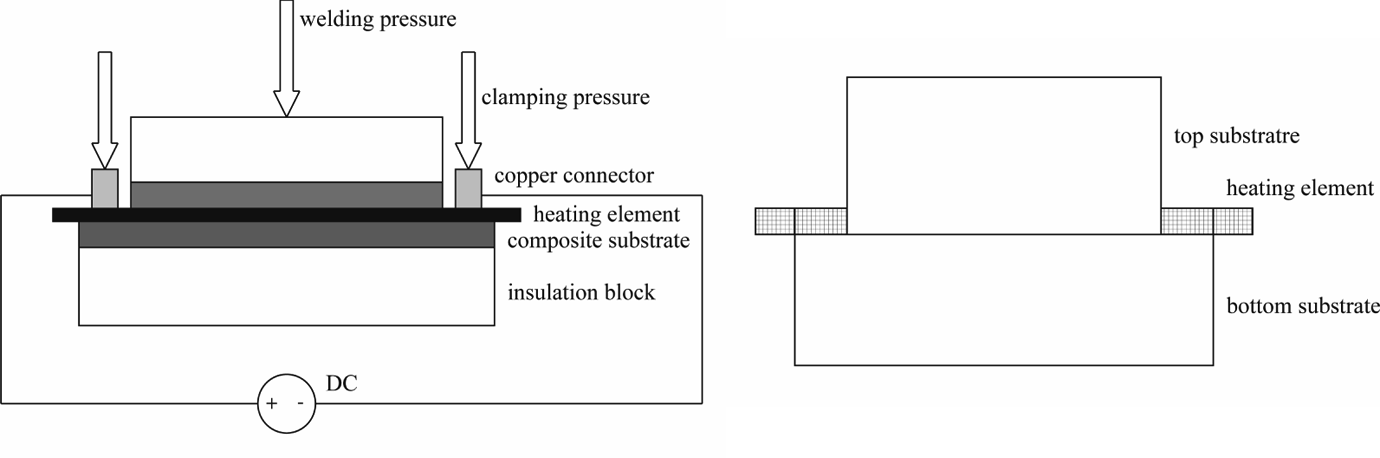
Schematic representation of the resistance welding set-up (left) and of the joint configuration (right).

Modelling

One-dimensional finite-element heat transfer models were built in COMSOL Multiphysics to better understand the experimental results. One of them, referred to as the mesh model, consisted of a simplified mesh (solid heating element) with an insulated thermocouple on top to simulate the quasi-isothermal tests (Figure 5). The other one, referred to as the welding model, simulated a welding process with a simplified metal mesh embedded in resin, composite substrates and thermal insulation blocks. A half model with symmetry boundary conditions was used in this case to reduce the computational time. The simplified set of material properties used for the models is listed in Table 1. The governing heat transfer equation is the following

$\mathit{\rho }{C}_{\mathrm{p}}\frac{\mathrm{\partial }T}{\mathrm{\partial }t}=\dot{q}+k_{xx}\frac{{\mathrm{\partial }}^{2}T}{\mathrm{\partial }{x}^2}+k_{zz}\frac{{\mathrm{\partial }}^{2}T}{\mathrm{\partial }{z}^2};\dot{q}=\frac{I^{2}R\left(T\right)}{V}$

2

where ρ and C _p and k_xx and k_zz are the density and specific heat capacity and longitudinal and transverse thermal conductivity, respectively. $\dot{q}$ is the volumetric Joule heat generated by a mesh with temperature-dependent resistance R and volume V, and a constant current I.

Figure 5.

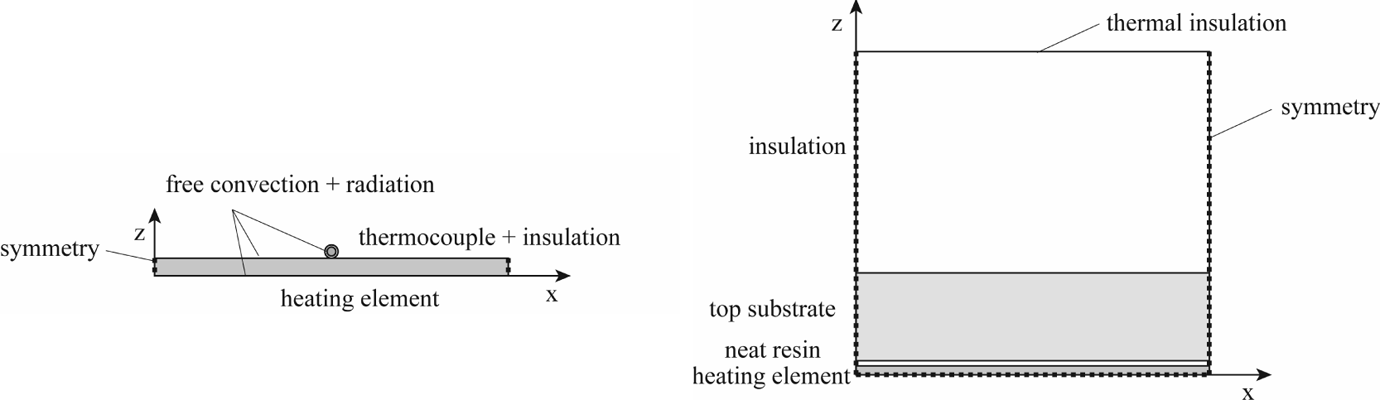
Unidimensional heat transfer models: mesh model (left) and welding model (right). Free convection to air coefficient h = 5 WK/m², surface emissivity ε = 0.95.

Table 1.

Material property values used for the unidimensional models

	ρ (kg/m3)	C p (J/kgK)	kxx (W/mK)	kzz (W/mK)
Neat PEIa	1281	980	0.23	0.23
Neat PPSb	1350	1090	0.19	0.19
GF/PEIc	1925	890	0.40	0.53
GF/PPSc	1900	900	0.40	0.53
304L meshd	7900	500	21.4	21.4
K-type thermocouplee	8800	460	60.7	60.7
Polyimide tapef	1420	1090	0.12	0.12
Woodf	1242	2400	0.17	0.17

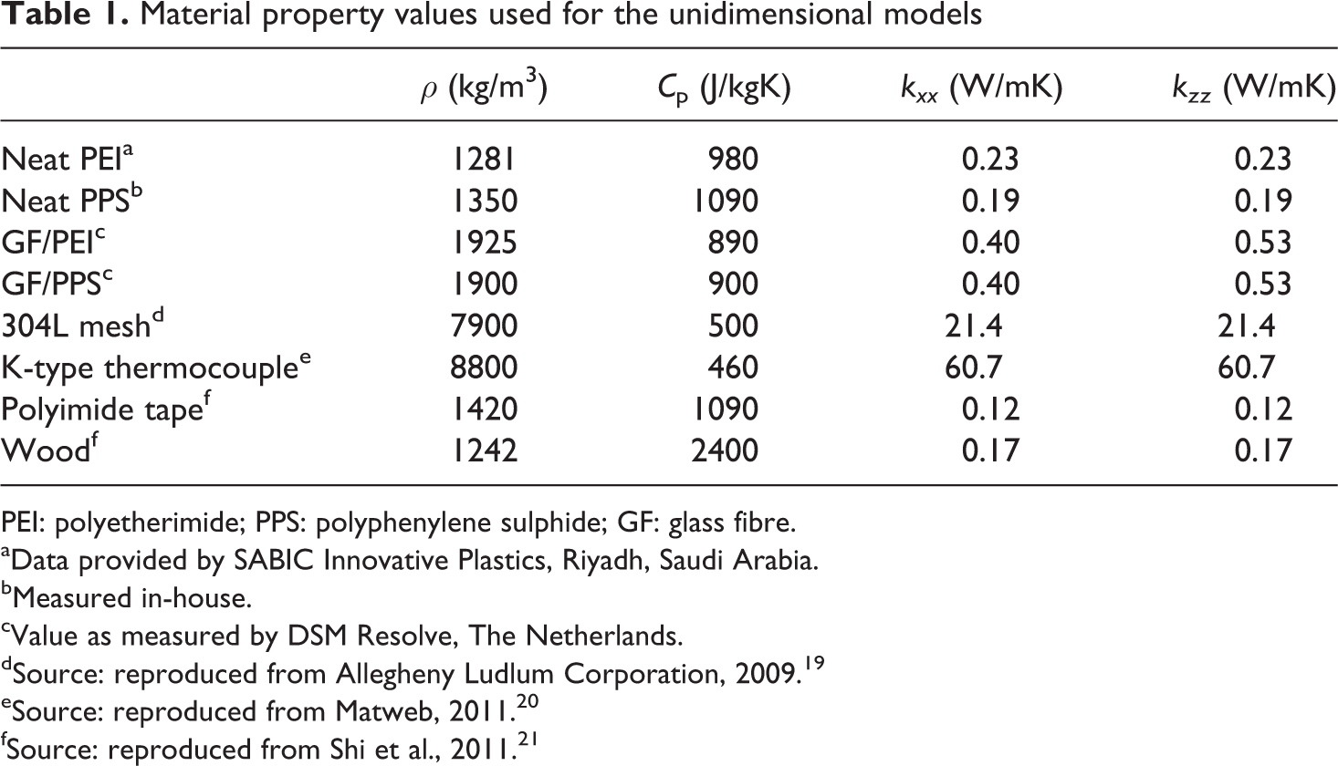
PEI: polyetherimide; PPS: polyphenylene sulphide; GF: glass fibre.

^aData provided by SABIC Innovative Plastics, Riyadh, Saudi Arabia.

^bMeasured in-house.

^cValue as measured by DSM Resolve, The Netherlands.

^dSource: reproduced from Allegheny Ludlum Corporation, 2009. ¹⁹

^eSource: reproduced from Matweb, 2011. ²⁰

^fSource: reproduced from Shi et al., 2011. ²¹

Results and discussion

Isothermal tests

The isothermal resistance measurements for both the single wire and the 12-wire mesh yielded linear resistance versus temperature curves, which hence could be described by the following equation: ¹⁴

$R=R_0\left(1+\mathit{\alpha }\left(T-T_0\right)\right)$

3

where α is the temperature coefficient of resistance at a reference temperature of 0°C (T ₀). The temperature coefficient calculated from the experimental results was for both the single wire and the mesh inside the same scatter region, quite broad in the case of the single wire probably due to deficiencies in the electrical connections (Table 2). Moreover, the resistance at 20°C of the 12-wire mesh coincided with that of the single wire divided by 12. This indicates the existence of no significant difference in potential along the transverse wires of the mesh, which results in the majority of the current flowing through the longitudinal wires.

Table 2.

Electrical characteristics of a single wire and a 12-wire metal mesh obtained from isothermal measurements.

	Number of experiments	R at 20°C (Ω) (c.o.v., %)	Temperature coefficient, α (K−1) for T 0 = 0°C (c.o.v., %)	R-squared linear fitting (c.o.v., %)
Single wire	3	5.39 (0.73)	8.57·10−4 (8.3)	0.997 (0.27)
12-Wire mesh	4	0.45 (2.11)	9.19·10−4 (2.3)	0.998 (0.06)

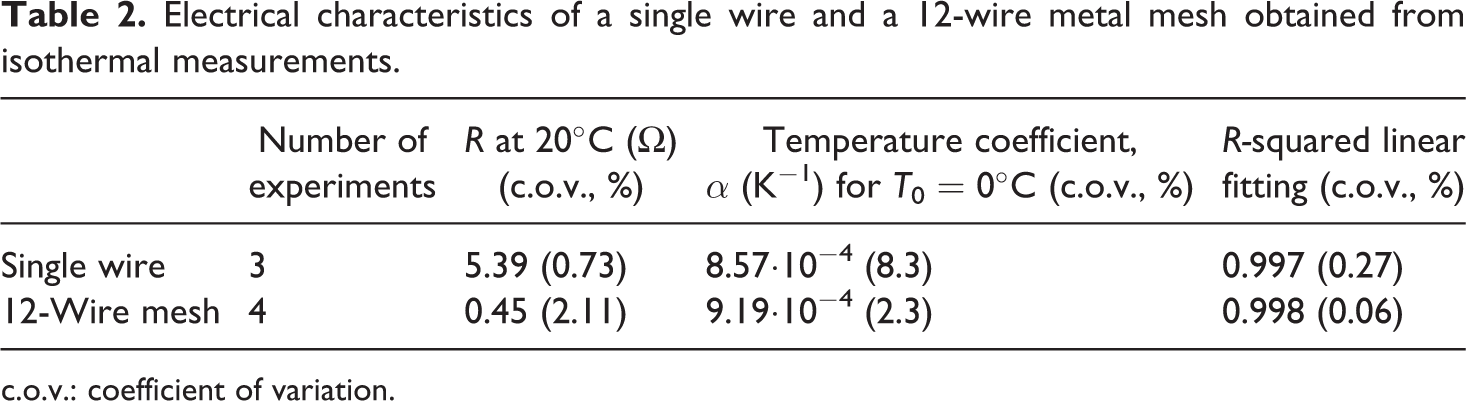
c.o.v.: coefficient of variation.

The temperature coefficient of resistivity available in the literature for 304L stainless steel is 10.4 × 10⁻⁴ K⁻¹, ²⁰ which is higher than the 8.57 × 10⁻⁴ K⁻¹ temperature coefficient of resistance obtained in these tests. The mismatch between resistivity and resistance coefficients caused by the thermal expansion of the wires (linear coefficient of thermal expansion of 19.8 × 10⁻⁶ m/mK^{−1 20}]) is however not big enough to account for this difference, which might result from variations in the testing methods. Nevertheless, the resistivity values at 20°C were substantially close, 7.03 × 10⁻⁵ Ωcm (experimental) versus 7.22 × 10⁻⁵ Ωcm (literature).

Quasi-isothermal tests

Figure 6 displays some of the transient resistance versus temperature data from quasi-isothermal measurements at three current levels. It shows non-linear resistance versus temperature relations associated with the very rapid temperature changes. The resistance of the mesh experiences a steep increase followed by a convergence to a constant value. Once this constant resistance is reached, the temperature continues to increase until it reaches equilibrium with the surroundings. Figure 7 shows the steady resistance and temperature data points at the end of the transient phase for all the measurements performed (referred to as quasi-isothermal R/T values).

Figure 6.

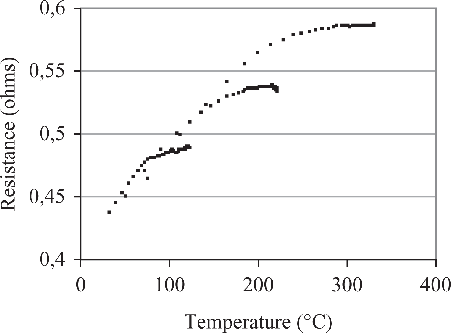
Transient resistance versus temperature measurements for 5, 7.5 and 10 A (from bottom to top).

Figure 7.

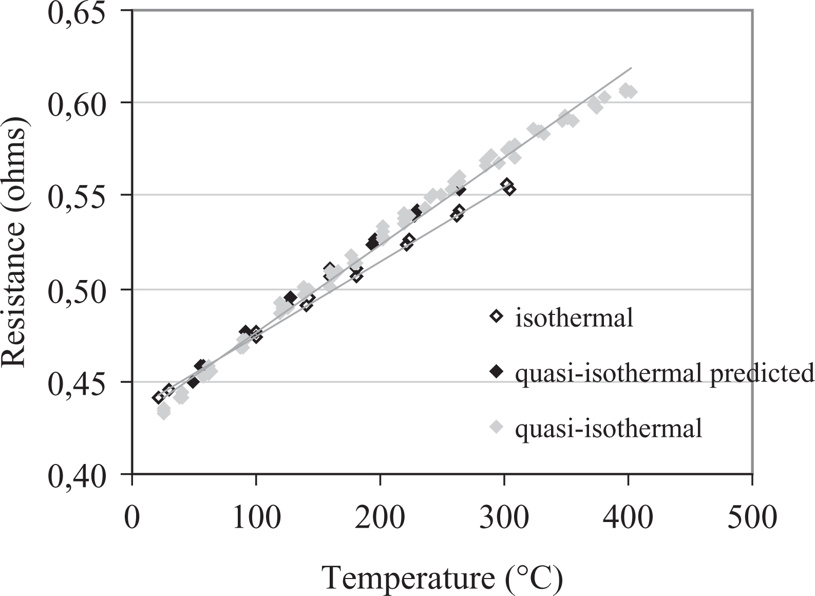
Quasi-isothermal resistance versus temperature measurements (experimental and predicted) when compared with the results from the isothermal tests (12-wire mesh).

Linear fitting of the quasi-isothermal resistance–temperature data led to an average resistance value at 20°C of 0.438 Ω (coefficient of variation (c.o.v.) 0.54%) and an average resistance temperature coefficient of 1.09 × 10⁻³ K⁻¹ (c.o.v. 1.91%). The resistance at 20°C is similar to the one measured in the isothermal tests, whereas the temperature coefficient is approximately 18% higher. These differences are caused by the high-transverse temperature gradients at the location of the thermocouples, which increase for higher mesh temperatures. As a result, the measured temperatures are lower than the actual ones, resulting in an apparently steeper resistance versus time relation and thus in a higher temperature coefficient. Figure 7 shows how the isothermal R/T curve falls onto the quasi-isothermal one when the isothermal temperatures are corrected with the temperatures at the location of the thermocouples resulting from the mesh model described in the ‘Modelling’ section.

In situ measurements

Shape of the resistance curves

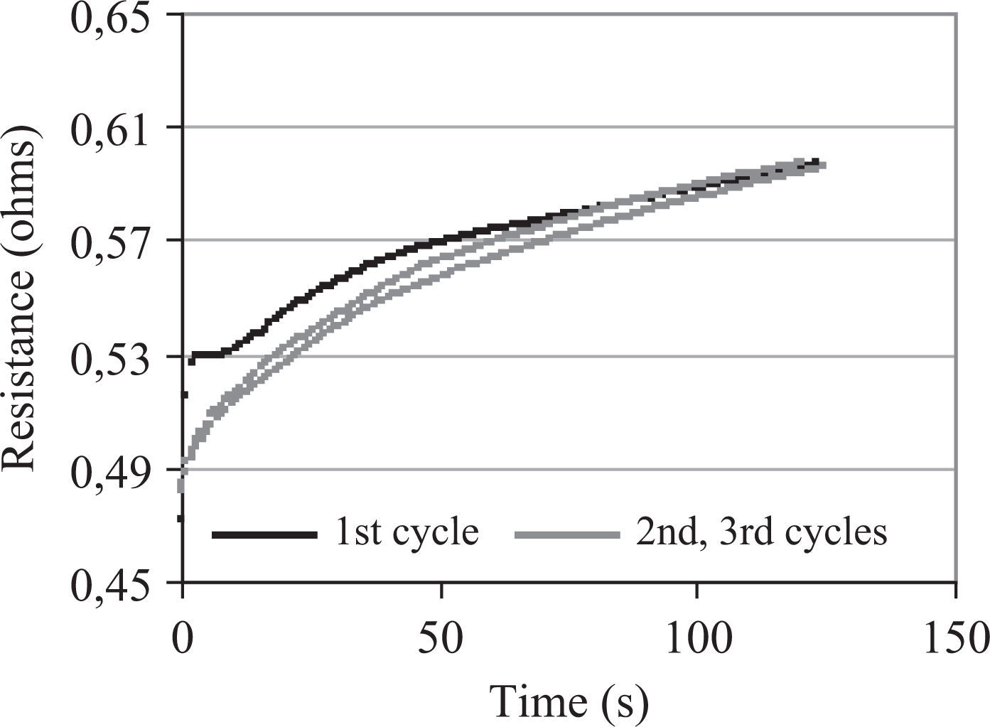
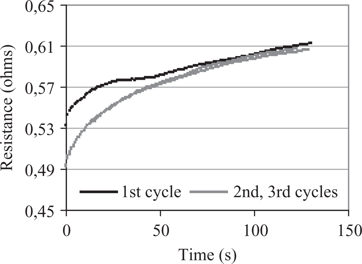
Figures 8 and 9 display representative resistance versus temperature plots for GF/PPS and GF/PEI welds with loose amorphous resin plies in the welding stack. ²² These figures show an approximately linear despite transient behaviour of the resistance of the mesh in the second and third welding cycles as a result of much lower heating rates than in the quasi-isothermal tests. The curves of the first welding cycle are, however, clearly non-linear. They show a resistance plateau in the vicinity of the glass transition temperature (T _g) of the matrix materials (90°C and 215°C for PPS and PEI, respectively) before tending to adopt the same quasi-linear trend as the second and third cycles. This convergence only happens beyond the melting temperature (T _m) of PPS, that is 280°C, for the GF/PPS welds and soon after the plateau in the case of the GF/PEI welds. The analysis of the resistance and temperature history indicated that such an anomalous behaviour was directly related to the resistance of the mesh itself (Figures 10 and 11). Some differences in average temperature were also registered at an initial stage between the first and the subsequent welding cycles, but they did not affect the shape of the temperature versus time curves and only amounted to a maximum of 20°C.

Figure 8.

Resistance versus temperature measurements during three consecutive welding cycles (15 A, GF/PPS substrates). GF: glass fibre; PPS: polyphenylene sulphide.

Figure 9.

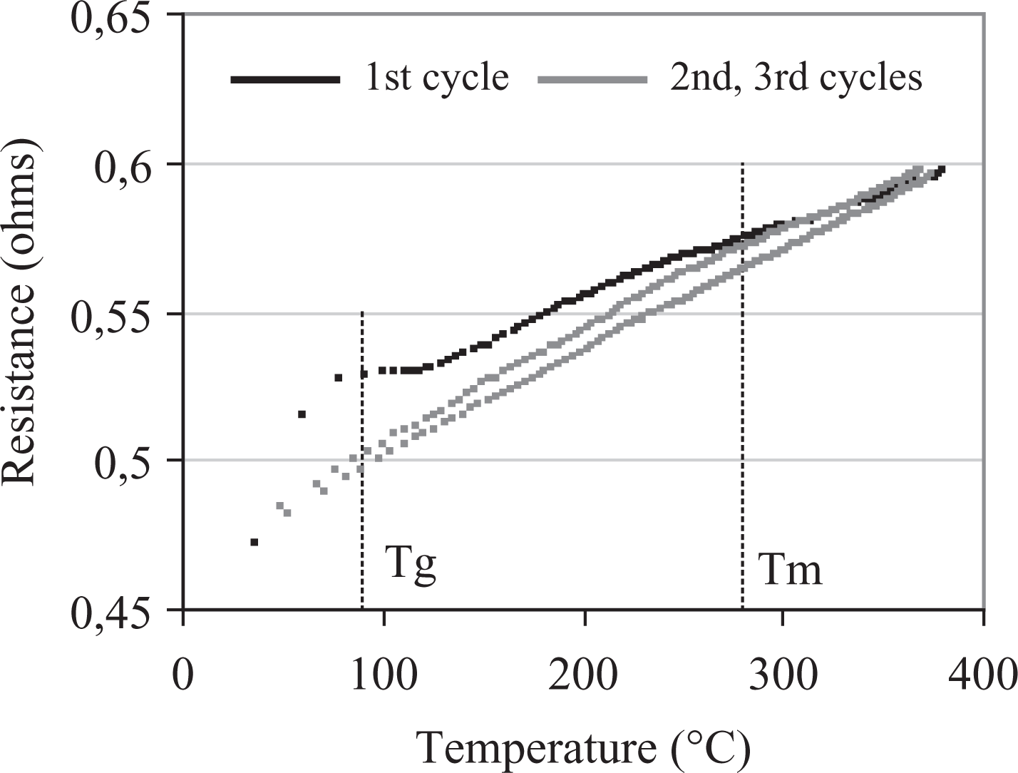
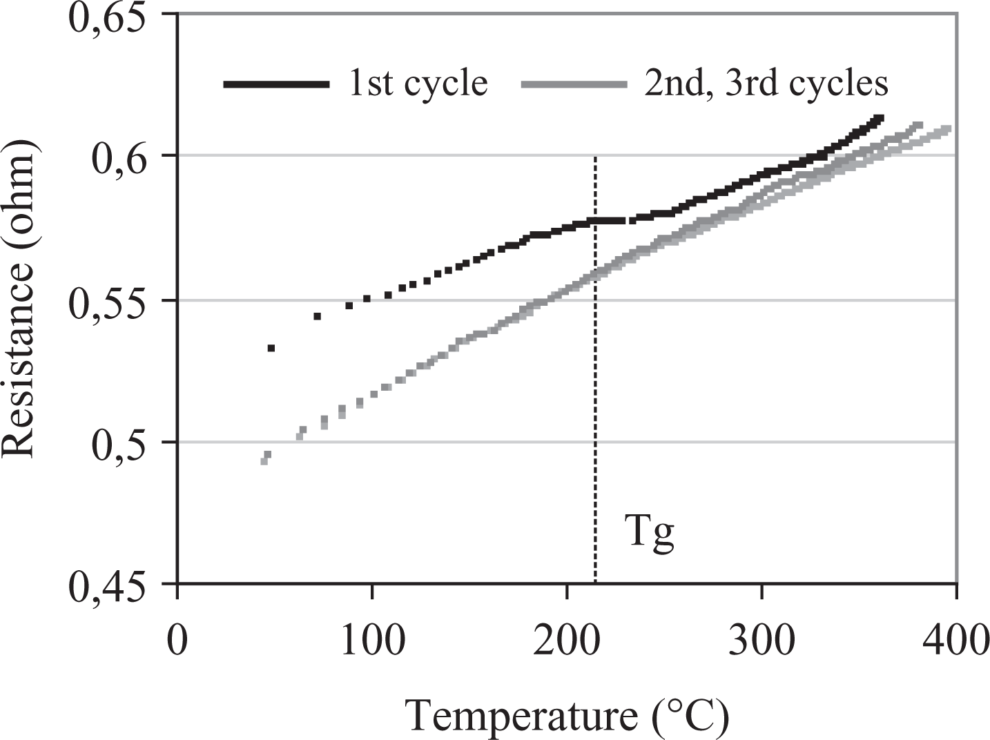
Resistance versus temperature measurements during three consecutive welding cycles (15 A, GF/PEI substrates). GF: glass fibre; PEI: polyetherimide.

Figure 10.

Evolution of the resistance of the mesh during three consecutive welding cycles (15 A, GF/PPS substrates). GF: glass fibre; PPS: polyphenylene sulphide.

Figure 11.

Evolution of the resistance of the mesh during three consecutive welding cycles (15 A, GF/PEI substrates). GF: glass fibre; PEI: polyetherimide

The explanation proposed by the authors for this atypical resistance behaviour is based on the changing heat transfer scenario around the mesh during the welding process. In a welding stack consisting of a heating element and adjacent neat resin plies, a big part of the total surface of the metal wires is initially in contact with air (Figure 12(a)). When current passes through the mesh, it will heat up fast and its resistance will tend to follow a non-linear evolution similar to the one shown in Figure 6. As the welding process progresses and the resin approaches its glass transition temperature, its stiffness will decrease and hence it will better conform to the wires of the mesh (Figure 12(b)). The heat loss from the mesh to the surrounding resin will increase as a result of the improved contact and will significantly lower the heating rate. Two counteracting effects will thus influence the transient resistance of the mesh: on the one hand, the tendency to increase with increasing temperature and on the other hand, the tendency to approach a quasi-isothermal behaviour due to a decreased heating rate. These opposed results explain the resistance plateau observed around the glass transition of the resin. At the optimum welding temperature, the resin flow will have eventually squeezed all the air out of the welding interface resulting in a completely embedded heating element (Figure 12(c)). This accounts for the final convergence of all the resistance curves.

Figure 12.

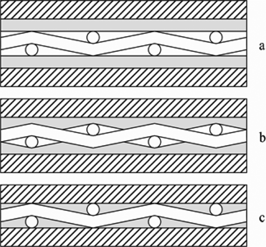
Progressive morphology changes in the resin plies surrounding the mesh that cause changes in the overall heat transfer rate: (a) initial state, (b) softening of the matrix material beyond its T _g and (c) mesh completely embedded in resin at the processing temperature.

Additional welding experiments further confirmed this hypothesis. When the metal mesh was sandwiched between semi-crystalline instead of amorphous PPS plies, the shape of the first welding curve was found to be different than the one in Figure 8. As shown in Figure 13, the evolution of the resistance was characterized by a steep rise at the beginning of the welding cycle and no clear plateau in the vicinity of the T _g of the matrix material. Convergence between the first and the subsequent welding curves was observed beyond the melting temperature of PPS. If, on the contrary, the heating element was pre-impregnated with PEI or PPS matrix resin and no thermocouples were used, no resistance differences could be found between the first and following welding cycles. This is explained by the fact that the metal wires were totally embedded in resin during the whole cycle, so no significant changes in the heat transfer scenario occurred. Nonetheless, when thermocouples were placed on the impregnated heating element, a separation with the substrate/substrates was created and therefore changing heat transfer scenarios were induced, which resulted in resistance curves similar to the ones in Figures 8 to 11.

Figure 13.

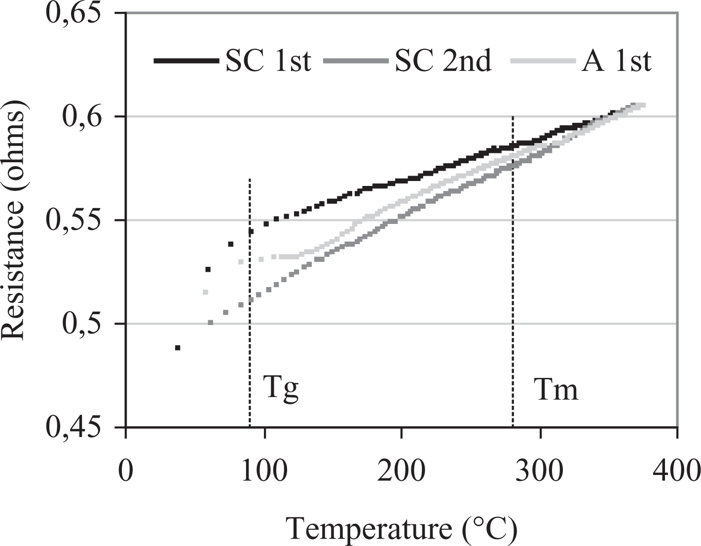
Resistance versus temperature curves of a mesh sandwiched in semi-crystalline (SC) PPS plies when compared with amorphous (A) PPS plies (15 A). PPS: polyphenylene sulphide.

Slope comparison

Linear fitting of the resistance versus temperature curves of the second and third welding cycles provided the resistance and temperature coefficient values listed in Table 3 and displayed in Figure 14. The in situ resistance values were found to be higher than the isothermal ones for the whole temperature range. The in situ temperature coefficients were, on the other hand, around 25% lower than the isothermal temperature coefficient. Consequently, the gap between in situ and isothermal resistance decreased for increasing temperatures. A maximum resistance difference of 0.040 Ω was calculated at 20°C, which was reduced to 0.015 Ω at 320°C.

Figure 14.

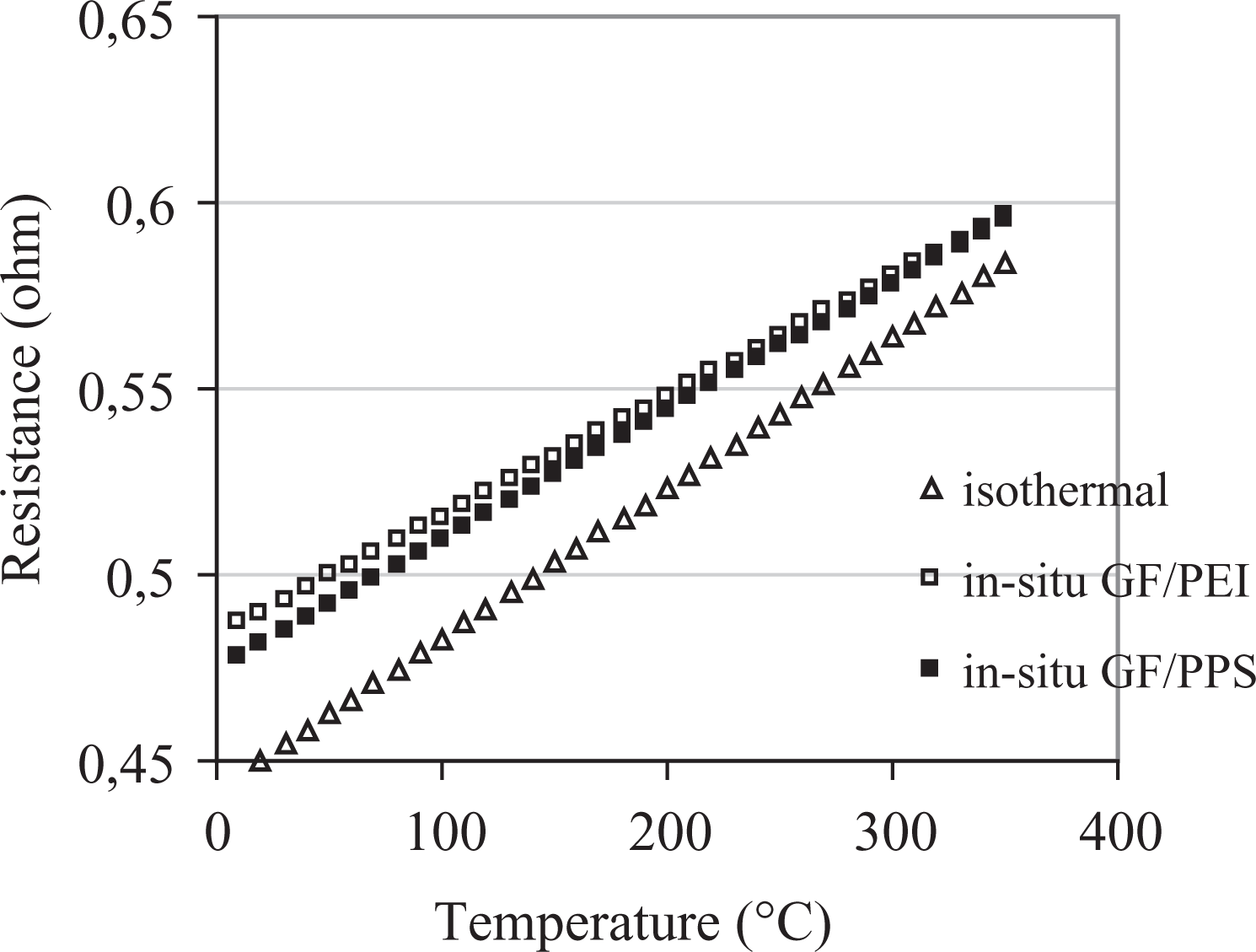
Linear interpolation for the resistance versus temperature relation in in situ and isothermal tests.

Several factors are believed to cause the higher in situ resistance values. First, the connections of the metal mesh heating element to the power supply unit introduce an extra resistance in the measuring circuit. Second, the temperature gradient through the neat resin surrounding the metal mesh causes the thermocouples to register a temperature below the one right on the metal wires. This gradient has a similar effect on the R/T relation as the one observed in the quasi-isothermal measurements, that is, higher resistance for a given measured temperature (Figure 7). Finally, the in situ R/T relation is obtained in transient conditions which, according to the results plotted in Figure 6, can be expected to result in higher resistance values, especially at the beginning of the process. As the process progresses and the heating rates decrease, the gap between transient and isothermal resistance will tend to decrease as seen in Figure 14. Another factor that causes differences between the in situ and isothermal resistance values is non-uniform temperature distributions at the weld line, which is generally observed in resistance welding of thermoplastic composites and strongly depends on the welding set-up. ¹⁹

It must be noted that, as opposed to the isothermal R/T relation, there is no universal in situ R/T relation for a certain heating element as a result of its dependence on non-isothermal and transient effects. As an example, the small differences in the temperature coefficients of GF/PPS and GF/PEI in situ tests are attributed to differences in the heat transfer capabilities of both resins.

Table 3.

Initial resistance and temperature coefficient values for the in situ (embedded mesh), quasi-isothermal and isothermal tests.

Type of test	Number of experiments	R at 20°C (Ω) (c.o.v., %) (extrapolated)	Temperature coefficient, α (K−1) for T 0 = 0°C (c.o.v, %)	R-squared linear fitting (c.o.v, %)
In situ GF/PPS	6	0.482 (1.03)	7.25·10−4 (2.28)	0.996 (0.26)
In situ GF/PEI	6	0.490 (1.40)	6.65·10−4 (4.24)	0.996 (0.14)
Quasi-isothermal	5	0.438 (0.54)	10.9·10−4 (1.91)	0.993 (0.24)
Isothermal (mesh)	4	0.450 (2.11)	9.19·10−4 (2.30)	0.998 (0.06)

PEI: polyetherimide; PPS: polyphenylene sulphide; GF: glass fibre; c.o.v.: coefficient of variation.

Closed-loop welding

The procedure proposed for closed-loop resistance welding based solely on resistance measurements is as follows. Once in the welding set-up, the electrical resistance of the heating element is measured at room temperature (R _RT) by introducing small current in it. This current needs to be small enough to ensure that the heating element remains at room temperature. The resistance at room temperature and a suitable R/T relation are then used to calculate the resistance of the heating element at the welding temperature, R _W, which is used as a target by the process-control routine. Among all the R/T relations derived in this work, the in situ one is a priori the most appropriate for closed-loop welding, since it relates the resistance of the mesh to the temperature of the resin in the welding stack during the actual process. The fairly linear shape of the in situ R/T curve in the surroundings of the processing temperature should make it possible to derive R _W from equation (3), even when the heating element is not pre-embedded in resin. However, predicting R _W from R _RT and the in situ temperature coefficient in Table 3 is not feasible since the initial resistance that would allow building an in situ R/T curve like the one in Figure 14 is notably affected by transient effects as discussed in ‘Slope comparison’ section. Yet the tendency of the in situ R/T curves to converge with the isothermal one at high temperatures makes it possible to use R _RT and the isothermal temperature coefficient to quite accurately predict R _W.

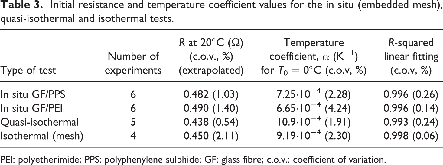
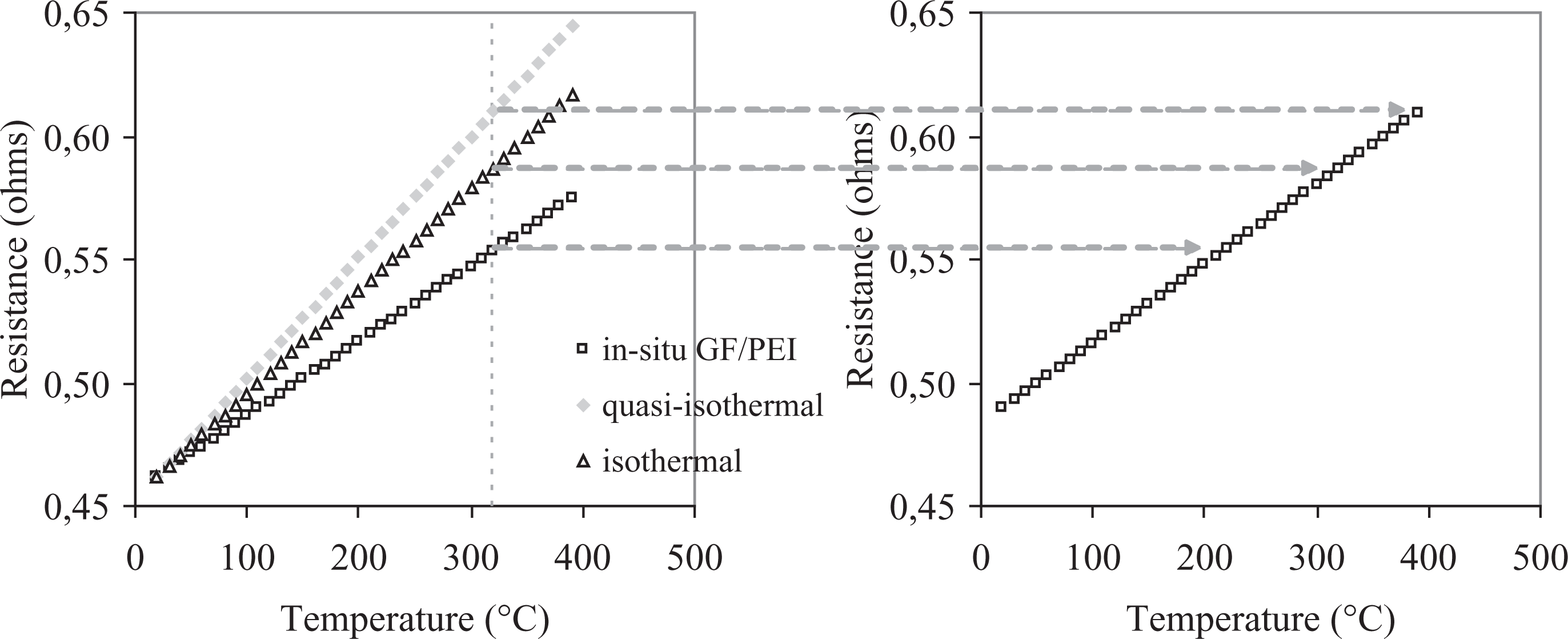
As an example, Figure 15 and Table 4 show the R _W values obtained from equation (3) for a nominal welding temperature of 320°C, a typical R _RT value of 0.462 Ω at 20°C (average resistance measured in the welding set-up for 40 different heating elements, ²³ c.o.v. 2.1%) and the isothermal, quasi-isothermal and GF/PEI in situ temperature coefficients. The actual welding temperatures corresponding to these R _W values as predicted by the GF/PEI in situ R/T curve in Figure 14 are also shown in Figure 15 and Table 4. As indicated above, the use of R _RT and the isothermal α leads to an actual welding temperature similar to the nominal one. On the contrary, the use of any of the other two temperature coefficients leads to either not enough heating (in situ α) or severe overheating (quasi-isothermal α). In addition, Figure 16 shows a cross-section micrograph of a good-quality GF/PEI sample welded in a closed-loop process based on the isothermal R/T relation with a nominal welding temperature of 320°C. The resulting welding time (around 70s for 17 A) was found to fall within the limits of the processing window as defined by Stavrov and Bersee ¹⁵ for the same material and welding set-up.

Figure 15.

Calculation of target resistance values based on an initial resistance of 0.462 Ω and different α values (left). Actual temperatures for the target resistance values based on the in situ R/T relation for GF/PEI in Figure 14 (right). GF: glass fibre; PEI: polyetherimide.

Figure 16.

Cross section micrograph (left) and resistance versus time graph (right) of a GF/PEI sample welded in a closed-loop resistance process based on the isothermal R/T relation (temperature set-point = 320°C). Resistance at room temperature = 0.467 Ω, resistance target = 0.588 Ω (dotted line in resistance graph). Current = 17 A. ²³ PEI: polyetherimide; GF: glass fibre.

Table 4.

Predicted resistance at a nominal welding temperature of 320°C from a reference resistance of 0.462 Ω at 20°C and different temperature coefficients along with the corresponding actual welding temperatures (based on in situ GF/PEI measurements).

α	R at 20°C (Ω)	R at 320°C (Ω)	Actual T (°C)
In situ GF/PEI	0.462	0.553	216
Quasi-isothermal	0.462	0.610	393
Isothermal (mesh)	0.462	0.587	321

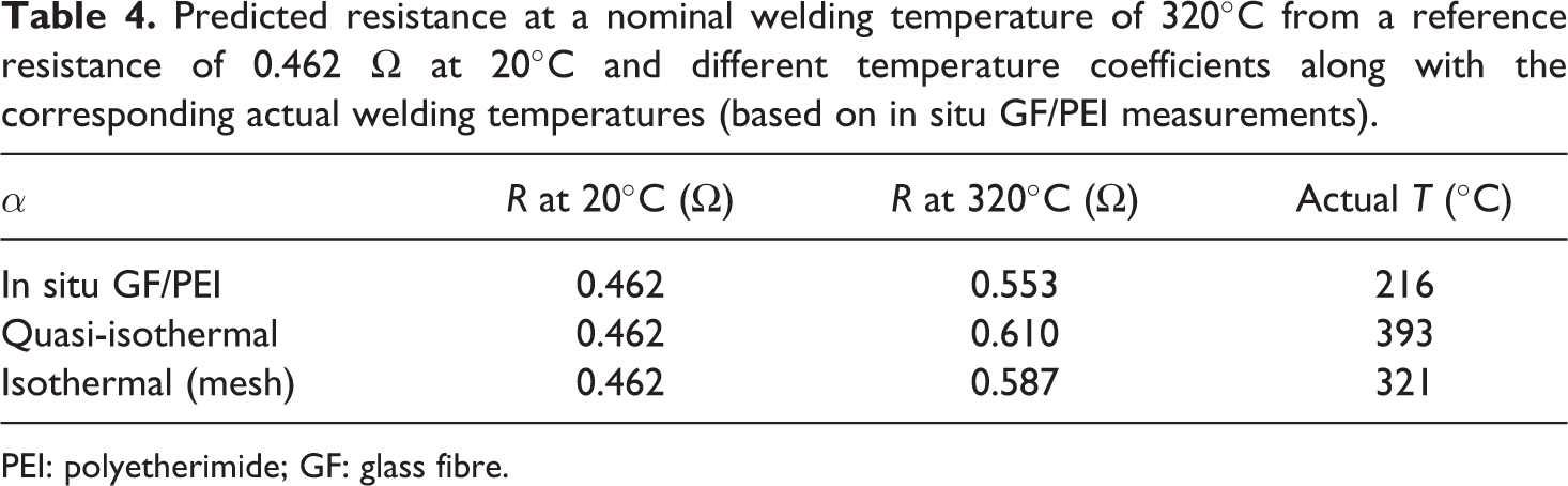
PEI: polyetherimide; GF: glass fibre.

Despite these results, it must be taken into account that the use of resistance measurements for closed-loop resistance welding has several limitations. First, non-isothermal and transient effects have an effect on the difference between the in situ and the isothermal R/T relations. Therefore, the error associated with the prediction of actual welding temperatures through an isothermal R/T relation is dependent on the welding configuration (materials, insulation, geometry, etc.). Second, the temperature distribution at the weld line is generally not uniform. As a result, the use of an average resistance value to control the process must be accompanied by knowledge on the typical temperature profiles for a certain welding set-up to ensure that the process temperatures are within the desired range.

Consequently, the definition of the processing conditions for each new welding set-up cannot be simplified to the point where just a target temperature and an isothermal R/T relation, only dependent on the nature of the heating element, need to be defined to determine the optimum welding time for a certain input power. Further information on the actual temperature profiles at the weld line is necessary to ensure high quality joints. Nevertheless, closed-loop welding based on resistance measurements enables the implementation of temperature controlled processes where, for instance, the processing temperature dwells for a certain time to improve uniformity. Likewise, monitoring of the resistance of the heating element during welding can be utilised as a helpful tool for online monitoring of the quality of the joints.

Conclusions

The evolution of the resistance at high temperatures of a stainless steel mesh heating element was investigated for its application to closed-loop welding based on indirect temperature feedback. Isothermal and quasi-isothermal resistance versus temperature curves were obtained based on external and on Joule heating of bare heating elements, respectively. The resistance of the heating element during actual welding of GF/PEI and GF/PPS composites was monitored and evaluated as well (in situ tests).

Fairly linear R/T relations were obtained in the three cases but with notably different resistance temperature coefficients as a result of temperature gradients and transient effects. During in situ tests, non-linear behaviour was observed at the beginning of the heating cycle if the mesh was not pre-embedded in the resin. This phenomenon, caused by changing heat transfer scenarios related to the physical changes in the resin, however did not cause deviations from linearity in the surroundings of the welding temperature.

Despite the fact that the in situ tests reproduced actual welding conditions, the isothermal R/T relation proved to be the most suitable one for the definition of closed-loop welding processes. The use of either the quasi-isothermal or the in situ temperature coefficients together with the resistance of the mesh at room temperature led to considerable temperature deviations with a large impact on the welding process.

Even though an isothermal R/T relation, which is dependent on the nature of the heating element, was successfully used in this investigation to control the resistance welding process in an application case, the error between the actual and the predicted temperatures is dependent on the welding set-up. Consequently, closed-loop welding based on resistance measurements still requires knowledge on the temperature distributions at the welding interface for each new welding configuration to ensure high-quality welds and thus it does not significantly simplify the definition of processing windows. However, it enables temperature-controlled welding processes and is a very useful tool for online quality monitoring.