Sage Journals: Discover world-class research

Abstract

The El Niño-Southern Oscillation (ENSO) is a profound climatic and oceanographic phenomenon arising from the thermal contrast between the western and eastern Pacific Ocean, and has far-reaching influences on ocean heat distribution, monsoonal rainfall and thermal structure of the water column in the Pacific Ocean. The East China Sea (ECS) is a marginal sea in the western Pacific, significantly influenced by the Kuroshio Current (KC), which originates from the West Pacific Warm Pool. The warm and saline water transported by KC determines the surface-to-subsurface oceanographic conditions, including the thermocline structure of the ECS. Downcore variability of the thermocline-sensitive planktic foraminifera over ~400 ka at IODP Site U1429 has been considered to decipher the linkage of ENSO-like processes and the thermocline structure in the ECS. Singular Value Decomposition (SVD) analysis was applied to major thermocline planktic foraminiferal (Neogloboquadrina dutertrei, Globoconella inflata, and Pulleniatina obliquiloculata) abundance data to extract three modes representing three distinct palaeoclimate signals. Trend-synchronisation tests were carried out to study the linear/non-linear relationship between obtained SVD modes, KC strength, SST, Salinity, Insolation variability and paleo-ENSO Proxy. SVD Mode 1 corresponds to KC subsurface intrusion, Mode 2 represents KC-induced seasonal upwelling, and Mode 3 is found to be linked with the residual signal of ENSO-like processes in the ECS. This study reveals that stronger KC during interglacial phases (MIS 9, 7, and 5) corresponds to La Niña-like conditions, which deepens the thermocline as indicated by thermocline species P. obliquiloculata. The intensification of La Niña-like conditions in the ECS occurred during the last 150 ka, with no effect of local insolation on the thermocline depths in the ECS.

Keywords

ENSO Thermocline Depth East China Sea Planktic Foraminifera Kuroshio Current

INTRODUCTION

The El Niño-Southern Oscillation (ENSO) is an important driver of various climatic/oceanographic phenomena like the Indian/East Asian Monsoon (Mohanty et al., 2023, 2025; Qiao et al., 2023; Ujiié et al., 2016; Zhao et al., 2019), and thermocline variability in the Pacific Ocean (Jia et al., 2018; Qian et al., 2023; Sagawa et al., 2012; Zhang et al., 2021). The ENSO also influences the hydrological/oceanographic conditions of the western Pacific Ocean at interannual-decadal to millennial timescales (Stephens et al., 2018; Zhang et al., 2021). The West Pacific Warm Pool (WPWP), acting as an active ocean heat sink in the equatorial Pacific (Ujiié et al., 2016), has a direct linkage with the ENSO cycles (Koutavas et al., 2002; Stott et al., 2002; Wang et al., 2017). Furthermore, the WPWP thermocline depth exhibits a direct association with the Walker circulation intensity (de Garidel-Thoron et al., 2007; Ujiié et al., 2016), which is the primary driving force behind ENSO-like processes in the equatorial Pacific.

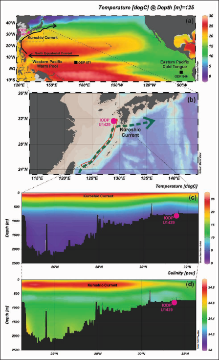
The Kuroshio Current (KC), originating from the western equatorial Pacific and flowing north-eastward, is an active conveyor of this equatorial heat and saline water from the WPWP to middle-latitudes (Hu et al., 2015), especially to the East China Sea (ECS) in modern day as well as over several glacial/interglacial cycles (Figure 1a and 1b, Ujiié et al., 2016; Vats et al., 2020). Such an intrusion of warm KC water to the Okinawa Trough of the ECS significantly affects the thermocline structure of the water column, and thus, stronger KC corresponds to deeper thermocline depths (Qian et al., 2023; Xiang et al., 2007). It implies that the ENSO has a significant influence on the ECS oceanographic conditions (Qiao et al., 2023), including the thermocline depths induced by KC intrusion (Qian et al., 2023). However, the implications of ENSO to the thermocline structure in the ECS remain poorly understood.

Figure 1.

(a) Map of the northern Pacific Ocean depicting the location of IODP Site U1429 (Magenta Circle), ODP Sites 871 and 846 (Black squares). The base map shows modern annual temperature (°C) distribution at 125 m depth (World Ocean Atlas 2023 dataset; Locarnini et al., 2024). Ocean currents are marked following Vats et al. (2020, 2021). (b) The red polygon in this figure, located along the Kuroshio Current, is used to depict the salinity and temperature profiles of the East China Sea (ECS). (c) Seawater temperature profile (Locarnini et al., 2024). (d) Salinity profile (Reagan et al., 2024) in the Okinawa trough of the ECS from the World Ocean Atlas 2023 dataset. The distribution map and cross-section profiles are made using Ocean Data View software (ODV 5.8.1, Schlitzer, 2025).

Modern-day ENSO variability accounts for the cyclic thermal contrast between the eastern and western tropical regions occurring at 2–7-year intervals. Similarly, ENSO-like processes at millennial to orbital scales also refer to the thermal contrast of the tropical Pacific Ocean. Although numerous studies, including those cited above, explain the modern-day linkage of ENSO with ECS oceanography (northwestern Pacific region), the long-term ENSO-induced thermocline variability in the ECS during glacial/interglacial phases remains unclear. The most recent studies by Qian et al. (2023) and Ujiié et al. (2003) explain this linkage, as it has only been observed over the last ~21 ka, due to the temporal constraint on the availability of high-resolution proxy records. Planktic foraminiferal species sensitive towards thermocline changes can resolve the implications of ENSO-like processes in the ECS. Hence, this study aims to decipher the linkages between paleo-ENSO variability and thermocline structure of the ECS water column during glacial/interglacial phases since the last 400 kyr, using planktic foraminiferal proxies.

STUDY LOCATION

The ECS is a marginal sea located in the mid-latitudes of the northwestern Pacific, and its oceanography responds to climate variability associated with KC inflow and East Asian Summer Monsoon (EASM) (Liu et al., 2021; Matsuzaki et al., 2019). The KC is the most prominent hydrological feature of the ECS (Qian et al., 2023). It is a warm and saline surface current originating from the North Equatorial Current in the North Pacific region (Figure 1a and 1b; Liu et al., 2021; Tomczak & Godfrey, 1994). The intrusion of KC into ECS is regulated seasonally due to fluctuations in the Kuroshio mainstream and volume transport (Liu et al., 2021). The permanent thermocline depth in the ECS lies at 150–550 m water depth and fluctuates due to strengthening or weakening of KC (Oka & Kawabe, 1998). The Yangtze/Changjiang River freshwater discharge from the EASM rainfall (Chen et al., 1994; Kubota et al., 2015) also significantly influences the Sea Surface Temperature (SST) and Sea Surface Salinity (SSS) of the ECS (Kubota et al., 2010) besides the KC influx.

The downcore planktic foraminiferal abundance from the composite sediment core (182 m) for the last 400 kyr (~2 kyr resolution) at Integrated Ocean Drilling Programme (IODP) Site U1429 (31°37.04ʹN, 128°59.85ʹE) has been used for the present study. The age model for the studied core was published by Clemens et al. (2018) and was further constrained by Vats et al. (2020) using AMS ¹⁴C dates for the last ~42 ka. The IODP Site U1429 is located on the western continental slope of the northern Okinawa Trough in the Danjo Basin at 732 mbsl in the northern ECS (Figure 1a and 1b). High sedimentation rates from riverine influx promote rapid burial and preservation of foraminiferal tests at the Site U1429, and any significant signs of differential dissolution of tests were not observed through microscopic examination. Although the ECS is sensitive to glacio-eustatic changes, owing to its location in the Okinawa Trough, Site U1429 has remained above sea level during the last 400 ka (Matsuzaki et al., 2019). The SST and SSS are 26°C and 32‰, respectively, near the studied site under modern-day conditions (Figure 1c and 1d; Matsuzaki et al., 2019).

MATERIALS AND METHODS

The major thermocline depth indicator planktic foraminiferal absolute counts are used from IODP Site U1429 (Vats et al., 2020). Species present at >10% abundance in five or more samples were considered for further analysis. The major thermocline-dwelling planktic foraminifera in the ECS include Neogloboquadrina dutertrei, Globoconella inflata (Lam & Leckie, 2020) (previously known as Globorotalia inflata), and Pulleniatina obliquiloculata. These species respond to KC strength and occur along with surface-dwelling species Globigerinoides ruber in the ECS (Vats et al., 2020). The population abundance data of these species were first detrended to remove any noise and then standardised prior to statistical analysis. Singular Value Decomposition (SVD) analysis was performed on the detrended and standardised dataset using MATLAB (R2024b). The SVD technique extracts underlying climate signals from the dataset by reducing noise and clarifying the relationships between species and their environments.

The Zonal (West–East) SST gradient between the WPWP and Eastern Pacific Cold Tongue has previously been used as a paleo-ENSO Proxy to understand the dynamics of ENSO forcing in the Equatorial Pacific Ocean at the millennial scale (de Garidel-Thoron et al., 2005; Jia et al., 2018; Zhao et al., 2019). Previously, Dyez and Ravelo (2013) had reconstructed planktic foraminiferal Mg/Ca-based SST from ODP Site 871 in the WPWP at ~3 kyr resolution, and Dyez et al. (2016) had published the interpolated alkenone-based U^k’₃₇-SST at 1 kyr resolution from ODP Site 846 in Eastern Pacific Cold Tongue. Therefore, we calculated the Zonal SST gradient as an ENSO Proxy by subtracting the Eastern Pacific Cold Tongue SST (Site 846) from the WPWP interpolated SST (Site 871) over the last 400 ka. An increase/decrease in the Zonal SST gradient indicates La Niña/El Niño conditions in the Pacific Ocean.

The other proxy data used in this study include Factor 4 loadings from Vats et al. (2020) representing KC strength, local δ¹⁸O_Seawater representing salinity variations and foraminiferal Mg/Ca-based SST in the ECS (Clemens et al., 2018). Insolation data between 20°N and 32°N (extent of KC intrusion in the ECS) for the last 400 ka at 1 kyr resolution was generated using Laskar solution La2010d (Laskar et al., 2011) in the Acyle MATLAB programme (Li et al., 2019).

A palaeoclimate dataset can have linear (initial assumption) and non-linear relationships or trends embedded within it, which often contain artefacts/noises due to irregular sampling, age-model uncertainty, calibration uncertainty, and the sensitivity of different proxies to climate forcing. This complicates the comparison to ascertain the linear relationship between the proxy variables (Franke & Donner, 2019). Therefore, to assess the trends and reveal the underlying relationship between all the proxy datasets along with the obtained SVD modes, trend-synchronisation tests like Linear Trend Synchronisation (LTS) using linear regression method, Dynamic Time Warping (DTW) distance, Trend Similarity Index (TSI), and Cross-Correlation of trends were performed using MATLAB. The LTS analysis has been used to understand the linear relationships between the proxies, while DTW, TSI, and Cross-Correlation have been carried out to assess the non-linear relationship between the proxies (Annexure I, Supplementary Material). Our default assumption of a linear relation between palaeoclimate records precedes the idea of non-linear relationships. Therefore, we initially considered the linearity test results for simplicity and tractability. In case of poor linearity test results only, we considered the non-linearity test results for robust palaeoclimate understanding. We address the issue of varying sample resolution by linearly interpolating all high-resolution datasets to a consistent 1-kyr time step. This enables a robust and direct comparison of different proxies, which is crucial for statistical analysis. The moving average window (kyr) was set to 100 for orbital-scale trend extraction. For the present study, the maximum lag for cross-correlation was set to 1 kyr to perform strict synchronous analysis.

RESULTS

The SVD allowed us to retain three modes corresponding to three distinct climate signals, which explain the complete (100%) variance of the dataset (Figure 2a) of major thermocline planktic foraminiferal species. The species contribution (significant contribution considered if the value is ~0.5) of each mode is presented in Figure 2b.

Figure 2.

(a) Plot of cumulative variance explained by Singular Value Decomposition (SVD) modes. (b) Plot of species contribution to Mode 1, 2 and 3.

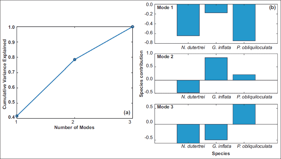
Mode 1 is characterised by a high negative contribution from both N. dutertrei and P. obliquiloculata (Figure 2b). Mode 1 loadings increase from 396 to 280 ka, show steady fluctuations between 280 and 130 ka, decrease between 130 and 110 ka, then again increase between 110 and 60 ka, and finally decline during 60-0 ka (Figure 3a).

Figure 3.

Time series plot of Singular Value Decomposition (SVD): (a) Mode 1, (b) Mode 2, and (c) Mode 3 over the last 400 ka. The grey bars represent even glacial MIS stages.

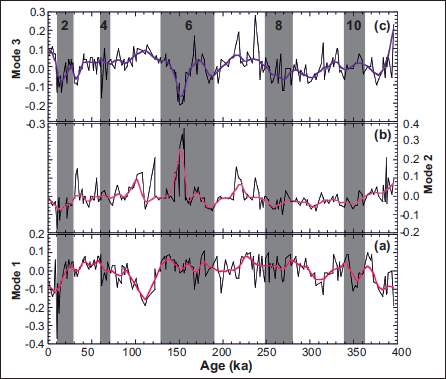
Mode 2 has only one species (G. inflata) with a contribution greater than 0.5 (Figure 2b) and exhibits peaks at 220 ka, 150 ka, and 100 ka, followed by a decline from 100 ka to the recent period (Figure 3b).

Mode 3 confers P. obliquiloculata with a high positive and N. dutertrei with a negative contribution, and a slight negative contribution from G. inflata. Mode 3 loadings decline from 396 ka to 380 ka, shows sporadic fluctuation between 380 and 270 ka, increases from 270 to 220 ka, declines from 220 to 150 ka with a small peak at 170 ka, increases from 150 ka 110 ka, then again decline between 110 and 10 ka, and finally shows increasing trend up to 0 ka (Figure 3c).

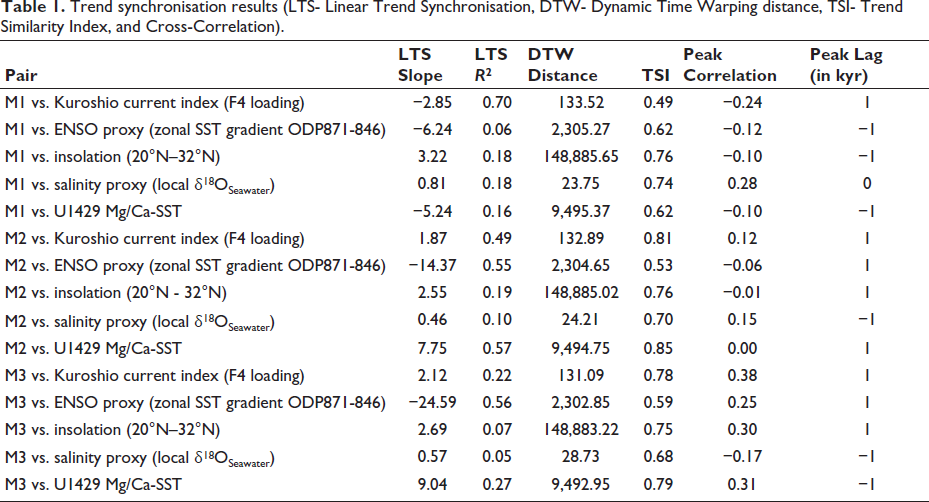
The trend-synchronisation test results for assessing the linear/non-linear relationships between the obtained SVD modes against KC Index-F4 Loading (Vats et al., 2020), ENSO Proxy (Zonal SST gradient ODP871-846), Insolation between 20°N and 32°N (Laskar et al., 2011), salinity proxy-local δ¹⁸O_Seawater, and U1429 Mg/Ca-SST (Clemens et al., 2018) have been presented in Table 1.

Table 1.

Trend synchronisation results (LTS- Linear Trend Synchronisation, DTW- Dynamic Time Warping distance, TSI- Trend Similarity Index, and Cross-Correlation).

Pair	LTS Slope	LTS R²	DTW Distance	TSI	Peak Correlation	Peak Lag (in kyr)
M1 vs. Kuroshio current index (F4 loading)	−2.85	0.70	133.52	0.49	−0.24	1
M1 vs. ENSO proxy (zonal SST gradient ODP871-846)	−6.24	0.06	2,305.27	0.62	−0.12	−1
M1 vs. insolation (20°N–32°N)	3.22	0.18	148,885.65	0.76	−0.10	−1
M1 vs. salinity proxy (local δ¹⁸O_Seawater)	0.81	0.18	23.75	0.74	0.28	0
M1 vs. U1429 Mg/Ca-SST	−5.24	0.16	9,495.37	0.62	−0.10	−1
M2 vs. Kuroshio current index (F4 loading)	1.87	0.49	132.89	0.81	0.12	1
M2 vs. ENSO proxy (zonal SST gradient ODP871-846)	−14.37	0.55	2,304.65	0.53	−0.06	1
M2 vs. insolation (20°N - 32°N)	2.55	0.19	148,885.02	0.76	−0.01	1
M2 vs. salinity proxy (local δ¹⁸O_Seawater)	0.46	0.10	24.21	0.70	0.15	−1
M2 vs. U1429 Mg/Ca-SST	7.75	0.57	9,494.75	0.85	0.00	1
M3 vs. Kuroshio current index (F4 loading)	2.12	0.22	131.09	0.78	0.38	1
M3 vs. ENSO proxy (zonal SST gradient ODP871-846)	−24.59	0.56	2,302.85	0.59	0.25	1
M3 vs. insolation (20°N–32°N)	2.69	0.07	148,883.22	0.75	0.30	1
M3 vs. salinity proxy (local δ¹⁸O_Seawater)	0.57	0.05	28.73	0.68	−0.17	−1
M3 vs. U1429 Mg/Ca-SST	9.04	0.27	9,492.95	0.79	0.31	−1

DISCUSSION

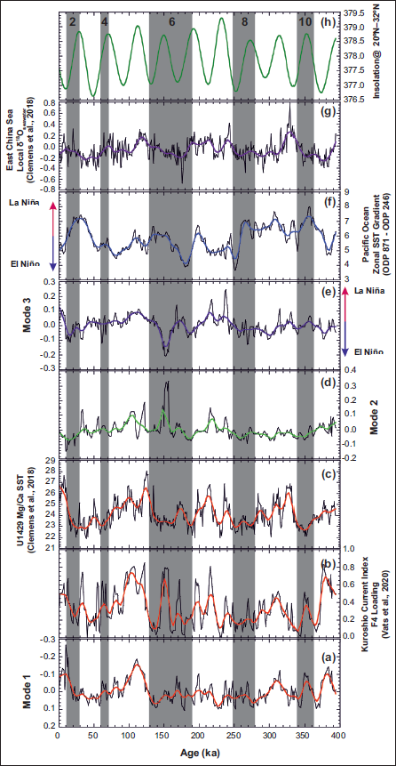
The previous reconstruction of the KC by Vats et al. (2020) discussed the surface-to-subsurface intrusion in the ECS. It included a combined assemblage of surface to mixed layer and thermocline planktic foraminifera, from which the thermocline response of planktic foraminifera in accordance with ENSO-like processes could not be ascertained. The SVD modes and proxy identities (KC strength, SST, Salinity, Insolation, and ENSO; Figure 4) focused on assessing the linear/non-linear and synchronous (±1 kyr) relationships between the proxies for paleoceanographic implications.

Figure 4.

Timeseries plot of (a) Mode 1, (b) Kuroshio Current Index- F4 Loading (Vats et al., 2020), (c) U1429 Mg/Ca-SST (Clemens et al., 2018), (d) Mode 2, (e) Mode 3, (f) ENSO Proxy (Zonal SST gradient ODP871-846), (g) Salinity Proxy- East China Sea Local δ¹⁸O_Seawater (Clemens et al., 2018), and (h) Insolation at 20°N - 32°N (Laskar et al., 2011) up to 394 ka interpolated at a 1 kyr resolution. The grey bars represent even MIS stages. The bold curves are a smoothed curve fit (4%) using KaleidaGraph software.

Response of thermocline planktic foraminifera

Mode 1 comprises two species (N. dutertrei and P. obliquiloculata) with a very high negative contribution (Figure 2b). N. dutertrei preferentially dwells in the upper to middle thermocline depths (40–70 m) (Rippert et al., 2015). This species is associated with the seasonal Deep Chlorophyll Maximum (Spero et al., 2003), which is found in the transitional area of KC extension (Vats et al., 2020). Sediment trap experiments in the ECS reveal maximum influxes of N. dutertrei during wintertime (Yamasaki & Oda, 2003), which may introduce a seasonal bias. Sporadic occurrences of N. dutertrei during 395–240 ka and 20–10 ka are observed in the downcore sediment samples at Site U1429 in the ECS (Figure 5a). P. obliquiloculata has been reported in tropical to subtropical areas of the Pacific-Indian Oceans (Bé, 1977), thriving in the surface to deep thermocline depths of 50–100 m (Dang et al., 2018; Rippert et al., 2015), and considered as KC and thermocline indicator species in the ECS (Baohua et al., 1997; Ujiié et al., 2016; Vats et al., 2020). P. obliquiloculata is also found to be associated with Deep Chlorophyll Maximum (Bé & Tolderlund, 1971). The overall abundance of P. obliquiloculata exhibits a declining trend from 396 to 130 ka, with some peaks during glacial/interglacial phases, an increase in abundance between 130 and 100 ka, and then a decline to 10 ka (Figure 5b). Both species (N. dutertrei and P. obliquiloculata) closely follow the reverse trend (LTS Slope of −2.85, Table 1) of Mode 1 (Figure 5a–5c) and have very high LTS R² (0.70) against KC Index-F4 Loading (Table 1). Therefore, Mode 1 is inferred as representative of KC subsurface intrusion in the ECS as it closely follows the trend of KC Index-F4 Loading and U1429 Mg/Ca-SST over the last 400 ka (Figure 4a–4c). The KC intrusion, variability and strength in the ECS have already been discussed in detail by Vats et al. (2020). Mode 1 also exhibits a moderate non-linear relationship with SST variability/ENSO-like processes in the ECS (TSI values of 0.62 for U1429 Mg/Ca-SST and the Zonal SST gradient, ODP871-846; Table 1). It exhibits a strong non-linear relationship with insolation variability (TSI > 0.7, Table 1), indicating that ENSO-like processes may also modulate N. dutertrei abundance in the ECS via non-linear thresholds. Mode 1 shows low DTW distance (<100), high TSI values (>0.7) and zero peak lag (Table 1) with salinity proxy (Figure 4g) indicating a strong non-linear relationship and influence of salinity variation caused by the EASM-induced riverine influx on the population abundance of thermocline planktic foraminifera; thus, confirms monsoon-driven shifts in the N. dutertrei abundance.

Figure 5.

Percentage abundance of dominant thermocline planktic foraminiferal species and obtained SVD modes in the East China Sea at Site U1429: (a) Neogloboquadrina dutertrei, (b) Pulleniatina obliquiloculata, (c) Mode 1, (d) Globoconella inflata and (e) Mode 2. Grey bars represent even MIS stages. The bold curves represent a smoothed curve fit (4%) using KaleidaGraph software.

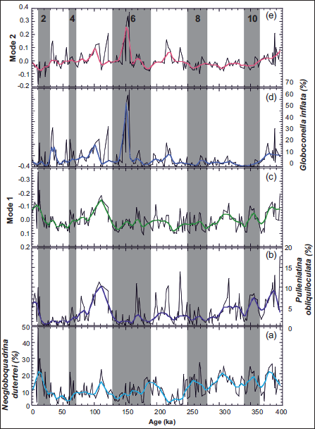
Mode 2 consisted of only one species (G. inflata), with a contribution greater than 0.5 (Figure 2b). G. inflata has been found in subpolar to subtropical latitudes in transitional water masses (Bé, 1977; Incarbona et al., 2019), reported as deep dwellers in the thermocline to intermediate water (Bé, 1977; Hemleben et al., 1989; Ujiié et al., 2016), abundant at 50 to 300 m depth (Mortyn & Charles, 2003), and associated with KC-related seasonal upwelling in the ECS (Vats et al., 2020). Downcore variability of G. inflata shows sporadic occurrence between 160 and 148 ka (Figure 5d). Mode 2 is inferred to be representative of subsurface upwelling of KC in the ECS (Figures 4d and 5e), as it exhibits a positive linear relationship with the KC Index-F4 Loading (LTS R² = 0.49, Table 1). A positive lag of +1 year with KC Index (F4 Loading), LTS R² of 0.55 with ENSO Proxy (Zonal SST gradient ODP871-846) and LTS R² of 0.57 with U1429 Mg/Ca-SST indicates that ENSO-like processes induce surface-to-subsurface temperature changes via KC intensification. This leads to subsurface KC upwelling, which influences the abundance of deep-dwelling species, such as G. inflata. Further, Mode 2 has a TSI value of 0.85 with U1429 Mg/Ca-SST, reinforcing that G. inflata tracks SST both linearly and nonlinearly, which also indicates that warming (increase in SST), typically due to KC intrusions, increased G. inflata abundance. Stronger KC during MIS 5 and MIS 7 may have caused an increase in the abundance of G. inflata during these periods (Vats et al., 2020). However, an anomalous peak at ~150 ka for Mode 3 variability and G. inflata abundance (Figures 4d, 5d and 5e) has been linked to EASM-induced coastal upwelling towards the warmer end of MIS 6 (Vats et al., 2020). This may explain its non-linear relationship with the salinity proxy, as indicated by the following criteria: High TSI value > 0.7 and Low DTW distance < 100 (Table 1). Apparently, Mode 2 also shares a non-linear relationship with insolation variability (Figure 4h; High TSI value >0.7, Table 1), which may indicate that G. inflata responds to secondary effects of northern hemisphere insolation-induced warm anomaly (Pahnke et al., 2003; Ujiié et al., 2016) in the ECS.

Response to ENSO-like processes

Mode 3 consists of P. obliquiloculata with a high positive and N. dutertrei with a negative contribution (Figure 2b). G. inflata also contributes negatively to this mode (Figure 2b). Contrasting contributions of P. obliquiloculata and N. dutertrei towards Mode 3 also suggest habitat differences between these two taxa (Ujiié et al., 2003; Xu & Oda, 1999). Abundances of N. dutertrei also correspond to the water of the subtropical gyre margin in the ECS apart from the KC water (Ujiié et al., 2003). Based on the ecological preferences and contrasting species contribution to Mode 3, and the LTS R² value of 0.56 against ENSO Proxy (Zonal SST gradient ODP871-846) (Table 1), Mode 3 is inferred as a representative residual signal of ENSO-like processes in the ECS.

Peaks of Mode 3 loading during MIS 9, 7, and 5 (Figure 4e) may have been linked to strengthening of the KC in the ECS (Vats et al., 2020) during La Niña phases. Stronger KC induces mixing of the upper water with the deep thermocline in modern-day conditions (Oka & Kawabe, 1998; Ujiié et al., 2016). Hence, MIS 9, 7, and 5 (Figure 4e) correspond to the formation of a deeper thermocline in the ECS, which supported thermocline species like P. obliquiloculata. The ENSO signal in the ECS (Mode 3 loadings) appears as a background forcing and does not show any prominent fluctuations from mid-MIS 11 to MIS 8 (Figure 4e). This supports the idea of transition from La Niña-like to El Niño-like conditions (Figure 4f) during this period (de Garidel-Thoron et al., 2005; Jia et al., 2018; Zhao et al., 2019). The negative contribution of G. inflata (Figure 2b) at ~150 ka is also evident in Mode 3 loadings, which suggest that an intense El Niño phase occurred during this time in the ECS. The El Niño phase led to poor stratification of the water column, associated with more vigorous EASM-led coastal upwelling, which supported the sudden increase in G. inflata abundance (Hilbrecht, 1996; Martínez et al., 2003; Zhao et al., 2019). Further, such an intense phase of El Niño-like conditions in the Equatorial Pacific Ocean results in weakening of the Kuroshio transport to the ECS (Ujiié et al., 2003; Vats et al., 2020). The increase in Mode 3 loading after ~150 ka, along with an increase in Zonal SST gradient records, suggests the intensification of La Niña-like conditions in the ECS, which has also been previously reported by Zhao et al. (2019).

The trend test results for Mode 3 against the U1429 Mg/Ca-SST (Slope = 9.04, R² = 0.27, Peak Correlation = 0.31 at a −1 kyr lag; Table 1), along with the positive contribution of P. obliquiloculata (Figure 2b), indicate that SST leads Mode 3 by 1 kyr. This suggests that SST-driven thermocline adjustments favour the moderate increase in P. obliquiloculata abundance in the ECS. Mode 3 exhibits a non-linear relationship with the KC Index - F4 Loading (TSI > 0.7, Peak Correlation = 0.38 at a +1 kyr lag; Table 1). It can be inferred that the KC strengthening deepens the thermocline in the ECS and favours the proliferation of P. obliquiloculata after the thermocline adjustment within 1 kyr. However, Mode 3 shows non-linearity (TSI = 0.68, DTW distance = 28.73) with the salinity proxy (Figure 4g), suggesting the role of EASM-induced riverine influx in shaping the thermocline of the ECS. The negative lag (−1 kyr) indicates that freshening (low salinity) of the ECS precedes P. obliquiloculata blooms due to monsoon-driven inputs in the ECS. Poor trend test results (Low LTS R² and a very high DTW distance of 148883.22) suggest that local insolation (between 20°N and 32°N) (Figure 4h) has no implications for the thermocline structure of the water column in the ECS.

CONCLUSION

The SVD analysis applied to major thermocline planktic foraminiferal (N. dutertrei, G. inflata, and P. obliquiloculata) abundance data allowed us to extract three modes representing three distinct palaeoclimate signals. Further, the linear/non-linear relationship between obtained SVD modes, KC strength, SST, Salinity, Insolation variability and paleo-ENSO Proxy (Zonal SST gradient from the Pacific Ocean) was evaluated using trend-synchronisation tests like LTS using linear regression method, DTW distance, TSI, and Cross-Correlation of trends. Based on environmental preference and trend-synchronisation tests, Mode 1 links with KC subsurface intrusion, Mode 2 with KC-induced seasonal upwelling, and Mode 3 with residual signal of ENSO-like processes in the ECS. Our study reveals that La Niña-like conditions deepen the thermocline in association with stronger KC in the ECS. This linkage supports the proliferation of thermocline species, such as P. obliquiloculata, during interglacial phases. ENSO-like processes stayed in a transition phase from La Niña-like to El Niño-like conditions during mid-MIS 11 to MIS 8. The intensification of La Niña-like conditions in the ECS has occurred only during the last 150 ka. This study further reveals that local insolation has no bearing on the thermocline levels in the ECS.

Footnotes

Acknowledgements

AKB, NV and SM thank IIT (ISM) Dhanbad for providing research facilities and NV thanks TEXMiN for providing the Postdoctoral Fellowship. RKS and MD thank IIT Bhubaneswar for providing research facilities.

Declaration of Conflicting Interests

The authors declared no potential conflicts of interest with respect to the research, authorship and/or publication of this article.

Funding

The authors received no financial support for the research, authorship and/or publication of this article.

Credit Authorship contribution statement

Nishant Vats: Writing – review & editing, Writing – original draft, Methodology, Investigation, Visualisation, Formal analysis, Data curation, Conceptualisation. Ajoy K. Bhaumik: Writing – review & editing, Investigation, Formal analysis. Manisha Das: Writing – review & editing, Investigation, Formal analysis. Satabdi Mohanty: Writing – review & editing, Investigation, Formal analysis. Raj K. Singh: Writing – review & editing, Investigation, Formal analysis.

Supplemental Material

ORCID iDs

Nishant Vats

Ajoy K. Bhaumik

Raj K. Singh

References

Baohua

, Zhimin

, & Pinxian

(1997). Pulleniatina obliquiloculata as a paleoceanographic indicator in the southern Okinawa trough during the last 20,000 years. Marine Micropaleontology , 32(1–2), 59–69. https://doi.org/10.1016/S0377-8398(97)00013-3

Bé

A. W. H.

(1977). An ecological, zoogeographic and taxonomic review of recent planktonic foraminifera. In

Ramsay

A. T. S.

(Ed.), Oceanic micropaleontology (Vol. 1, pp. 1–100). Academic Press. http://ci.nii.ac.jp/naid/10027957291/en/

Bé

A. W. H.

, & Tolderlund

D. S.

(1971). Distribution and ecology of living planktonic foraminifera in surface waters of the Atlantic and Indian Oceans. In

Funnel

B. M.

& Riedel

W. R.

(Eds.), The micropaleontology of oceans (pp. 105–149). Cambridge University Press.

Chen

, Beardsley

R. C.

, Limeburner

, & Kim

(1994). Comparison of winter and summer hydrographic observations in the Yellow and East China Seas and adjacent Kuroshio during 1986. Continental Shelf Research , 14(7–8), 909–929. https://doi.org/10.1016/0278-4343(94)90079-5

Clemens

S. C.

, Holbourn

, Kubota

, Lee

K. E.

, Liu

, Chen

, Nelson

, & Fox-Kemper

(2018). Precession-band variance missing from East Asian monsoon runoff. Nature Communications , 9(1), 3364. https://doi.org/10.1038/s41467-018-05814-0

Dang

, Jian

, Wu

, Bassinot

, Wang

, & Kissel

(2018). The calcification depth and Mg/Ca thermometry of Pulleniatina obliquiloculata in the tropical Indo-Pacific: A core-top study. Marine Micropaleontology , 145, 28–40. https://doi.org/10.1016/j.marmicro.2018.11.001

de Garidel-Thoron

, Rosenthal

, Bassinot

, & Beaufort

(2005). Stable sea surface temperatures in the western Pacific warm pool over the past 1.75 million years. Nature , 433(7023), 294–298. https://doi.org/10.1038/nature03189

de Garidel-Thoron

, Rosenthal

, Beaufort

, Bard

, Sonzogni

, & Mix

A. C.

(2007). A multiproxy assessment of the western equatorial Pacific hydrography during the last 30 kyr. Paleoceanography , 22(3). https://doi.org/10.1029/2006PA001269

Dyez

K. A.

, & Ravelo

A. C.

(2013). Late Pleistocene tropical Pacific temperature sensitivity to radiative greenhouse gas forcing. Geology , 41(1), 23–26. https://doi.org/10.1130/G33425.1

10.

Dyez

K. A.

, Ravelo

A. C.

, & Mix

A. C.

(2016). Evaluating drivers of Pleistocene eastern tropical Pacific sea surface temperature. Paleoceanography , 31(8), 1054–1069. https://doi.org/10.1002/2015PA002873

11.

Franke

J. G.

, & Donner

R. V.

(2019). Correlating palaeoclimate time series: Sources of uncertainty and potential pitfalls. Quaternary Science Reviews , 212, 69–79. https://doi.org/10.1016/j.quascirev.2019.03.017

12.

Hemleben

, Spindler

, & Anderson

O. R.

(1989). Modern planktonic foraminifera . Springer. https://doi.org/10.1007/978-1-4612-3544-6

13.

Hilbrecht

(1996). Extant planktic foraminifera and the physical environment in the Atlantic and Indian Oceans: An atlas based on CLIMAP and Levitus (1982) data (Vol. 300). Mitteilungen aus dem Geologischen Institut der ETH & Universität Zürich. http://www.fuhrmann-hilbrecht.de/Heinz/frame.html

14.

, Wu

, Cai

, Gupta

A. Sen

, Ganachaud

, Qiu

, Gordon

A. L.

, Lin

, Chen

, Hu

, Wang

, Sprintall

, Qu

, Kashino

, Wang

, & Kessler

W. S.

(2015). Pacific western boundary currents and their roles in climate. Nature , 522(7556), 299–308. https://doi.org/10.1038/nature14504

15.

Incarbona

, Jonkers

, Ferraro

, Sprovieri

, & Tranchida

(2019). Sea surface temperatures and paleoenvironmental variability in the central Mediterranean during historical times reconstructed using planktonic foraminifera. Paleoceanography and Paleoclimatology , 34(3), 394–408. https://doi.org/10.1029/2018PA003529

16.

Jia

, Li

, Xiong

, Steinke

, Jiang

, Chang

, & Qin

(2018). Hydrological variability in the western tropical Pacific over the past 700 kyr and its linkage to Northern Hemisphere climatic change. Palaeogeography, Palaeoclimatology, Palaeoecology , 493, 44–54. https://doi.org/10.1016/j.palaeo.2017.12.039

17.

Koutavas

, Lynch-Stieglitz

, Marchitto

T. M.

, & Sachs

J. P.

(2002). El Niño-like pattern in ice age tropical Pacific sea surface temperature. Science , 297(5579), 226–230. https://doi.org/10.1126/science.1072376

18.

Kubota

, Kimoto

, Tada

, Oda

, Yokoyama

, & Matsuzaki

(2010). Variations of East Asian summer monsoon since the last deglaciation based on Mg/Ca and oxygen isotope of planktic foraminifera in the northern East China Sea. Paleoceanography , 25(4), PA4205. https://doi.org/10.1029/2009PA001891

19.

Kubota

, Tada

, & Kimoto

(2015). Changes in East Asian summer monsoon precipitation during the Holocene deduced from a freshwater flux reconstruction of the Changjiang (Yangtze River) based on oxygen isotope mass balance in the northern East China Sea. Climate of the Past , 11, 265–275. https://doi.org/10.5194/cp-11-265-2015

20.

Lam

A. R.

, & Leckie

R. M.

(2020). Late Neogene and Quaternary diversity and taxonomy of subtropical to temperate planktic foraminifera across the Kuroshio Current Extension, northwest Pacific Ocean. Micropaleontology , 66(3), 177–268. https://doi.org/10.47894/mpal.66.3.01

21.

Laskar

, Fienga

, Gastineau

, & Manche

(2011). La2010: A new orbital solution for the long-term motion of the Earth. Astronomy & Astrophysics , 532, A89. https://doi.org/10.1051/0004-6361/201116836

22.

, Hinnov

, & Kump

(2019). Acycle: Time-series analysis software for palaeoclimate research and education. Computers & Geosciences , 127, 12–22. https://doi.org/10.1016/j.cageo.2019.02.011

23.

Liu

, Gan

, Hu

, Wu

, Cai

, & Deng

(2021). Progress of studies on circulation dynamics in the East China Sea: The Kuroshio exchanges with the shelf currents. Frontiers in Marine Science , 8. https://doi.org/10.3389/fmars.2021.620910

24.

Locarnini

R. A.

, Mishonov

A. V.

, Baranova

O. K.

, Reagan

J. R.

, Boyer

T. P.

, Seidov

, Wang

, Garcia

H. E.

, Bouchard

, Cross

S. L.

, Paver

C. R.

, & Dukhovskoy

(2024). World Ocean Atlas 2023, Volume 1: Temperature (Vol. 89, p. 52). In

Mishonov

(Ed.), NOAA Atlas NESDIS 89. https://doi.org/10.25923/54bh-1613

25.

Martínez

, Keigwin

, Barrows

T. T.

, Yokoyama

, & Southon

(2003). La Niña-like conditions in the eastern equatorial Pacific and a stronger Choco jet in the northern Andes during the last glaciation. Paleoceanography , 18(2). https://doi.org/10.1029/2002PA000877

26.

Matsuzaki

K. M.

, Itaki

, & Tada

(2019). Paleoceanographic changes in the northern East China Sea during the last 400 kyr as inferred from radiolarian assemblages (IODP Site U1429). Progress in Earth and Planetary Science , 6(1), 22. https://doi.org/10.1186/s40645-019-0256-3

27.

Mohanty

, Chaudhuri

, Bhaumik

A. K.

, & Kumar

(2023). Late-Holocene paleoceanographic and climatic changes and their impact on Indian socio-economic conditions: Benthic foraminiferal evidence from the Bay of Bengal. The Holocene , 33(7), 791–806. https://doi.org/10.1177/09596836231163505

28.

Mohanty

, Chaudhuri

, Chattopadhyay

, Patrick

N. M.

, Vats

, & Bhaumik

A. K.

(2025). Influence of monsoon variability on hydrographic and productivity dynamics in the western Bay of Bengal during the late Holocene: A planktic foraminiferal perspective. Palaeogeography, Palaeoclimatology, Palaeoecology , 670, 112971. https://doi.org/10.1016/j.palaeo.2025.112971

29.

Mortyn

P. G.

, & Charles

C. D.

(2003). Planktonic foraminiferal depth habitat and δ¹⁸O calibrations: Plankton tow results from the Atlantic sector of the Southern Ocean. Paleoceanography , 18(2). https://doi.org/10.1029/2001PA000637

30.

Oka

, & Kawabe

(1998). Characteristics of variations of water properties and density structure around the Kuroshio in the East China Sea. Journal of Oceanography , 54(6), 605–617. https://doi.org/10.1007/BF02823281

31.

Pahnke

, Zahn

, Elderfield

, & Schulz

(2003). 340,000-year centennial-scale marine record of southern hemisphere climatic oscillation. Science , 301(5635), 948–952. https://doi.org/10.1126/science.1084451

32.

Qian

, Chang

, Li

, Sun

, & Zhang

(2023). Thermocline variability in the subtropical northwestern Pacific since the last deglaciation. Palaeogeography, Palaeoclimatology, Palaeoecology , 612, 111379. https://doi.org/10.1016/j.palaeo.2022.111379

33.

Qiao

, Nakamura

, Tomita

, Kako

, Nishina

, Zhu

, & Liu

(2023). ENSO-related interannual variability of the Kuroshio in the East China Sea since the Mid-2000s. Journal of Geophysical Research: Oceans , 128(11). https://doi.org/10.1029/2023JC019749

34.

Reagan

J. R.

, Seidov

, Wang

, Dukhovskoy

, Boyer

T. P.

, Locarnini

R. A.

, Baranova

O. K.

, Mishonov

A. V.

, Garcia

H. E.

, Bouchard

, Cross

S. L.

, & Paver

C. R.

(2024). World Ocean Atlas 2023, Volume 2: Salinity (Vol. 90, p. 52). In

Mishonov

(Ed.), NOAA Atlas NESDIS 90. https://doi.org/10.25923/70qt-9574

35.

Rippert

, Baumann

K.-H.

, & Pätzold

(2015). Thermocline fluctuations in the western tropical Indian Ocean during the past 35 ka. Journal of Quaternary Science , 30(3), 201–210. https://doi.org/10.1002/jqs.2767

36.

Sagawa

, Yokoyama

, Ikehara

, & Kuwae

(2012). Shoaling of the western equatorial Pacific thermocline during the last glacial maximum inferred from multispecies temperature reconstruction of planktonic foraminifera. Palaeogeography, Palaeoclimatology, Palaeoecology , 346–347, 120–129. https://doi.org/10.1016/j.palaeo.2012.06.002

37.

Schlitzer

(2025). Ocean Data View (ODV 5.8.1) . https://odv.awi.de/

38.

Spero

H. J.

, Mielke

K. M.

, Kalve

E. M.

, Lea

D. W.

, & Pak

D. K.

(2003). Multispecies approach to reconstructing eastern equatorial Pacific thermocline hydrography during the past 360 kyr. Paleoceanography , 18(1), 1022. https://doi.org/10.1029/2002PA000814

39.

Stephens

G. L.

, Hakuba

M. Z.

, Webb

M. J.

, Lebsock

, Yue

, Kahn

B. H.

, Hristova-Veleva

, Rapp

A. D.

, Stubenrauch

C. J.

, Elsaesser

G. S.

, & Slingo

(2018). Regional intensification of the tropical hydrological cycle during ENSO. Geophysical Research Letters , 45(9), 4361–4370. https://doi.org/10.1029/2018GL077598

40.

Stott

, Poulsen

, Lund

, & Thunell

(2002). Super ENSO and global climate oscillations at millennial time scales. Science , 297(5579), 222–226. https://doi.org/10.1126/science.1071627

41.

Tomczak

, & Godfrey

J. S.

(1994). Regional oceanography . In Regional oceanography: An introduction. Elsevier. https://doi.org/10.1016/C2009-0-14825-0

42.

Ujiié

, Asahi

, Sagawa

, & Bassinot

(2016). Evolution of the North Pacific Subtropical Gyre during the past 190 kyr through the interaction of the Kuroshio Current with the surface and intermediate waters. Paleoceanography , 31(11), 1498–1513. https://doi.org/10.1002/2015PA002914

43.

Ujiié

, Ujiié

, Taira

, Nakamura

, & Oguri

(2003). Spatial and temporal variability of surface water in the Kuroshio source region, Pacific Ocean, over the past 21,000 years: Evidence from planktonic foraminifera. Marine Micropaleontology , 49(4), 335–364. https://doi.org/10.1016/S0377-8398(03)00062-8

44.

Vats

, Mishra

, Singh

R. K.

, Gupta

A. K.

, & Pandey

D. K.

(2020). Paleoceanographic changes in the East China Sea during the last ~400 kyr reconstructed using planktic foraminifera. Global and Planetary Change , 103, 173. https://doi.org/10.1016/j.gloplacha.2020.103173

45.

Vats

, Singh

R. K.

, Das

, Holbourn

, Gupta

A. K.

, Gallagher

S. J.

, & Pandey

D. K.

(2021). Linkages between East China Sea deep-sea oxygenation and variability in the East Asian summer monsoon and Kuroshio Current over the last 400,000 years. Paleoceanography and Paleoclimatology , 36, e2021PA004261. https://doi.org/10.1029/2021PA004261

46.

Wang

, Deser

, Yu

J.-Y.

, DiNezio

, & Clement

(2017). El Niño and Southern Oscillation (ENSO): A review. In Coral reefs of the eastern tropical Pacific: Persistence and loss in a dynamic environment (pp. 85–106). https://doi.org/10.1007/978-94-017-7499-4_4

47.

Xiang

, Sun

, Li

, Oppo

D. W.

, Chen

, & Zheng

(2007). Paleoenvironmental change in the middle Okinawa Trough since the last deglaciation: Evidence from the sedimentation rate and planktonic foraminiferal record. Palaeogeography, Palaeoclimatology, Palaeoecology , 243(3–4), 378–393. https://doi.org/10.1016/j.palaeo.2006.08.016

48.

, & Oda

(1999). Surface-water evolution of the eastern East China Sea during the last 36,000 years. Marine Geology , 156(1–4), 285–304. https://doi.org/10.1016/S0025-3227(98)00183-2

49.

Yamasaki

, & Oda

(2003). Sedimentation of planktonic foraminifera in the East China Sea: Evidence from a sediment trap experiment. Marine Micropaleontology , 49(1–2), 3–20. https://doi.org/10.1016/S0377-8398(03)00024-0

50.

Zhang

, Yu

, Gong

, Wang

, Chang

, Lohmman

, Qi

, & Li

(2021). Precession cycles of the El Niño/Southern Oscillation-like system controlled by Pacific upper-ocean stratification. Communications Earth & Environment , 2(1), 239. https://doi.org/10.1038/s43247-021-00305-5

51.

Zhao

, Wan

, Song

, Gong

, Zhai

, Shi

, & Li

(2019). Asynchronous variation in the Quaternary East Asian Winter Monsoon associated with the tropical Pacific ENSO-like system. Geophysical Research Letters , 46(12), 6955–6963. https://doi.org/10.1029/2019GL083033

Supplementary Material

Please find the following supplemental material available below.

For Open Access articles published under a Creative Commons License, all supplemental material carries the same license as the article it is associated with.

For non-Open Access articles published, all supplemental material carries a non-exclusive license, and permission requests for re-use of supplemental material or any part of supplemental material shall be sent directly to the copyright owner as specified in the copyright notice associated with the article.

0.00 MB

0.18 MB

Correspondence of ENSO-like processes to the thermocline planktic foraminifera in the East China Sea over the last 400 ka

Abstract

Keywords

INTRODUCTION

STUDY LOCATION

MATERIALS AND METHODS

RESULTS

(a) Plot of cumulative variance explained by Singular Value Decomposition (SVD) modes. (b) Plot of species contribution to Mode 1, 2 and 3.

Time series plot of Singular Value Decomposition (SVD): (a) Mode 1, (b) Mode 2, and (c) Mode 3 over the last 400 ka. The grey bars represent even glacial MIS stages.

Trend synchronisation results (LTS- Linear Trend Synchronisation, DTW- Dynamic Time Warping distance, TSI- Trend Similarity Index, and Cross-Correlation).

DISCUSSION

Response of thermocline planktic foraminifera

Response to ENSO-like processes

CONCLUSION

Footnotes

Acknowledgements

Declaration of Conflicting Interests

Funding

Credit Authorship contribution statement

Supplemental Material

ORCID iDs

References

Supplementary Material