
Abstract
Direct-demand (DD) models are used to estimate bicycle exposure (typically expressed as annual average daily bicycle volume [AADB]) when observed counts are unavailable at a site. The DD models typically estimate exposure as a function of site characteristics, such as the geometry, surrounding land use, and sociodemographic characteristics. Developing a DD model requires observed volume counts and associated site characteristics data for many sites in the target jurisdiction. In the absence of this data, it is desirable to apply a DD model from another jurisdiction. However, the naïve transferability of DD models results in AADB estimates with large errors. This paper investigates the use of calibration methods to enhance the spatial transferability of DD models to estimate bicycle volumes at intersections. This paper examined five DD models across four jurisdictions: (1) City of Milton (52 sites); (2) City of Toronto (28 sites); (3) Region of Waterloo (158 sites) in Canada; (4) Pima County (70 sites); and (6) Arizona, US, covering a total of 308 sites. Five local calibration techniques were evaluated for their effectiveness in mitigating errors in naïve estimates. The findings indicate that calibration, particularly regression-based methods, significantly improves the accuracy of the AADB predictions, with calibration Model 3 being the most effective for jurisdictions with less than 80 count sites (
Keywords
A measure of exposure is required as an input to most road safety analyses. Traditionally, only exposure of vehicles, frequently expressed as annual average daily traffic (AADT), has been used. However, with the increased focus on improving safety for vulnerable road users (VRUs, i.e., bicyclists and pedestrians), there is a need to have estimates of exposure for bicyclists and pedestrians as well as vehicles. When continuous counts (CCs) of VRUs are available, then the annual average traffic for VRUs can be directly calculated. When CCs are available only for a subset of sites and short-term counts (STCs) are available for the remaining sites, exposure can be estimated using a factor-based approach ( 1 , 2 ). For sites where neither CCs nor STCs are available, it has been proposed to apply direct-demand (DD) models ( 3 , 4 ), which estimate exposure as a function of site characteristics (e.g., geometry, surrounding land use, population demographics). In addition, statistical approaches such as DD models are common alternatives for estimating VRU exposure. The DD models have typically been regression models, but more recently, machine learning approaches have also been proposed ( 5 , 6 ). However, developing a DD model requires CCs from some sites in the jurisdiction, and studies suggest a minimum of at least 50–70 sites are required to develop a DD model ( 4 , 7 , 8 ). Furthermore, even when sufficient CCs are available, the local jurisdiction may not have the resources or expertise to develop the DD models. Using an existing DD model developed in another jurisdiction (i.e., spatially transferring) can be a practical alternative for estimating VRU exposure in the target jurisdiction ( 4 ).
The spatial transferability of existing DD models has been examined for pedestrians ( 4 ) and cyclists ( 9 ). The findings show that naïvely transferring DD models from other jurisdictions can result in large estimation errors (expressed as the average absolute error between the estimated and true counts for all sites in a jurisdiction divided by the average true count across all sites in the jurisdiction) from 0.52 to 50 for pedestrian exposure ( 4 ) and from 0.41 to 31.9 for bicyclist exposure ( 9 ). Furthermore, Soldouz and Hellinga ( 9 ) showed that naïvely transferring DD models developed in one jurisdiction to estimate bicyclist exposure in another jurisdiction produced estimation errors (quantified as the root mean squared exposure estimation error [RMSE] from 7–600 times larger than the RMSE associated with the original jurisdiction from which the DD model was developed. Significantly, Soldouz and Hellinga ( 9 ) also showed that there is only a weak correlation between measures of similarity between the development and target jurisdictions and the performance accuracy of the spatially transferred model. Therefore, selecting a DD model from a development jurisdiction that has similar levels of bicycling activity or similar site characteristics does not guarantee that the model will perform well in the target jurisdiction.
Sobreira and Hellinga ( 10 ) investigated and evaluated methods to improve the spatial transferability of DD models for estimating pedestrian exposure and found that these could improve (reduce) estimation errors by between 4.5% and 65% (compared with the naïve transferability method). Inspired by this previous work, the goal of this paper is to evaluate methods for improving the naïve transferability of existing DD models for bicycle exposure estimation at intersections. The next section summarizes the literature review. The Methodology section describes the estimation procedure for naïve transferability and the assessment of selected calibration methods. This is followed by the Results and Discussion section. Finally, the last section presents the conclusions and recommendations for future studies.
Literature Review
Spatial transferability in transportation engineering has been primarily explored in mode choice modeling ( 11 – 13 ). Transferability frameworks can be categorized in various ways, with the most common approach being naïve transferability. Although naïve transferability generally results in lower estimation accuracy, it can serve as a useful benchmark for evaluating other transferability calibration approaches ( 10 , 11 , 13 ).
Another major category is scaling approaches, with the most common being the adjustment of the original model’s parameters, estimates, and constants. Another scaling approach that has been used to transfer an already developed model involves retaining all parameters from the original model and adjusting the constant to calibrate it locally—also known as the alternative-specific constant ( 11 , 14 ). These approaches are practical because a locally calibrated model does not require collecting a complete data set from multiple sources to develop a model from scratch. Instead, it only requires data relevant to the already developed model, making the process more cost- and time-efficient.
This literature review section is divided into two sections. The first discusses previous work related to the spatial transferability of DD models for estimating VRU exposure. The second section presents DD models for estimating bicycle exposure.
Previous Work on Spatial Transferability of DD Models for Estimating VRU Exposure
Several studies have explored the spatial transferability of DD models used to estimate active transportation volumes, yielding mixed results ( 9 , 15 – 18 ). Wang et al. ( 15 ) found that DD models developed for Minneapolis, MN, and Columbus, Ohio, performed poorly when applied to the other city, with error rates 1.7 times higher than in their original contexts. More recent studies ( 16 , 18 ) explored the effect of combining static and crowdsourced data on model accuracy, finding that models incorporating both data types reduced error rates but still showed significant increases (up to 1.6 times) when applied across different locations or years within the same jurisdiction.
Existing research on the spatial transferability of DD models reveals mixed results, with transferred models showing errors 1.0–1.7 times higher than when applied within their original jurisdictions. These studies often rely on limited STCs to estimate the AADB, introducing inaccuracies, and use varied data sources that combine multi-use paths and roadway segments. Temporal and spatial transferability are frequently assessed together, complicating the isolation of spatial factors. Addressing these gaps, Soldouz and Hellinga ( 9 ) analyzed the transferability of five DD models across four jurisdictions using true AADB values, finding that applying models naively across regions leads to substantial estimation errors.
One study examines improving the naïve transferability of existing DD models for estimating annual average daily pedestrian traffic (AADPT) ( 10 ). This study proposed calibration methods that serve as a benchmark for this paper. That study proposed and evaluated five calibration methods to improve the naïve transferability of three DD models for estimating the AADPT. The three DD models used in this paper are in log-linear or negative binomial format as depicted in Equation 1.

where
The five local calibration models evaluated by Sobreira and Hellinga ( 10 ) are presented and described as follows.
Calibration Model 1
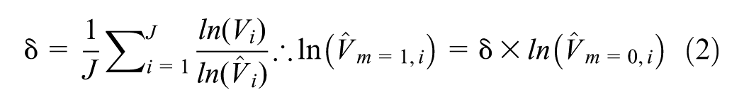
Calibration Model 2
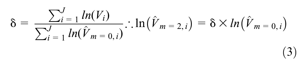
Calibration Model 3

Calibration Model 4

Calibration Model 5

where
The accuracy of the model estimates of the AADPT was quantified for each jurisdiction for the mean absolute error (MEA). (Equation 7), and the error indicator


There are two key findings from the study ( 10 ) that are relevant to this paper.
Locally calibrating DD models for estimating pedestrian exposure resulted in a substantial improvement in estimation accuracy (average of 35% reduction in estimation error).
Local calibration Models 2 and 3 were the best, with Model 2 performing better when CCs are available for less than 2.5% of all sites in the target jurisdiction and Model 3 otherwise.
DD Models for Estimating Bicycle Exposure
Building on the insights gained from pedestrian exposure modeling, Soldouz and Hellinga ( 9 ) reviewed existing DD models for estimating bicycle exposure. The goal of the review was to identify DD models that could be used to evaluate the spatial transferability of models. Therefore, only those models that were developed in jurisdictions within Canada or the US and contained explanatory variables for which values could be retrieved from open source data sets, such as census data, land use, and network data, and did not require STCs or crowdsourced information were considered. Five DD models were found that satisfied the previous criteria, and they are summarized in Table 1.
Summary of Selected Bicycle Volume Estimation Direct-Demand Models
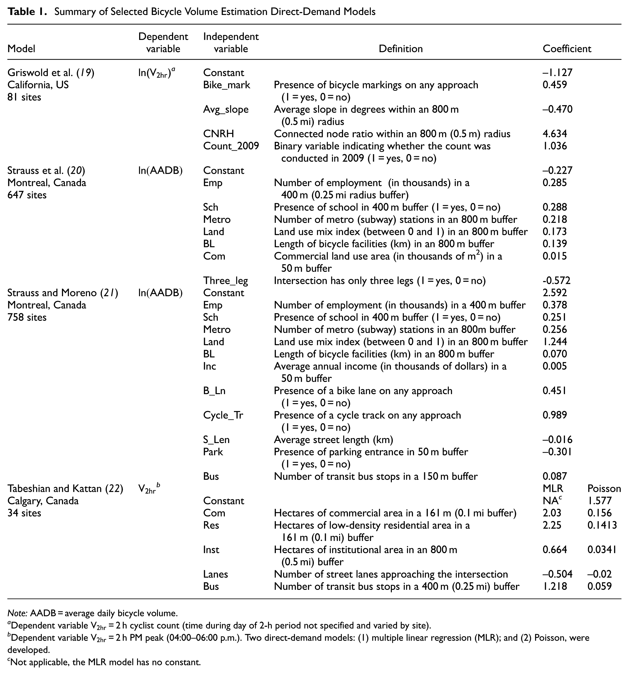
Note: AADB = average daily bicycle volume.
a
Dependent variable
b
Dependent variable
c Not applicable, the MLR model has no constant.
Four of the five selected models are log-linear models with a structure as depicted in Equation 9, and the remaining multiple linear regression (MLR) model by Tabeshian and Kattan ( 22 ) has a linear structure as depicted in Equation 10.


where
The next section describes the empirical data used to quantify the AADB estimation accuracy when naïvely transferring these five DD models to other jurisdictions. These results are the basis for assessing the accuracy improvements that can be provided by local calibration of spatially transferred DD models.
Data Description
A total of 308 signalized intersections were selected as target jurisdictions from the following locations: (1) 52 from the City of Milton, ON, Canada; (2)28 from the City of Toronto, ON, Canada; (3) 70 from Pima County, Arizona, US; and (4) 158 from the Region of Waterloo, ON, Canada. The bicycle volumes vary across these four jurisdictions. The CCs were obtained for a full year, between July 2023 and June 2024, by the same vendor for all four target jurisdictions, offering minute-by-minute bicycle counts for each turning movement and crossing at intersections using a camera-based data collection system. To validate bicycle count accuracy, manual counts and video recordings were collected during peak hours (04:30–6:30 p.m.) at a busy intersection in Toronto with an AADB = 4,000. Two analysts independently reviewed the video to produce manual counts, which averaged 672.5 and were the ground truth. The corresponding count from the vendor’s camera-based continuous count system was 675, demonstrating over 99% accuracy. This verification was limited to a single location and did not test different conditions, such as weather, intersection configuration, or sites with lower AADBs; the results suggest that the camera-based counts used in this paper are reliable for this analysis.
The data were aggregated to provide daily (24 h) counts for each day at each intersection, including all approaches. The counting system only reports data when a count is registered. Consequently, there is no distinction between instances where the system is not operating and when no users are traversing the intersection, as in both cases, no counts are reported. Therefore, in this paper, sites were included if: (1) the camera-based system was installed for the full 12-month period; and (2) there were no large gaps in the data collection (i.e., sites were excluded if no vehicle traffic was detected for more than four consecutive days). The true AADB count for each intersection was calculated using Equation 11.

where
Table 2 provides descriptive statistics for the true AADB of the selected intersections across the four target jurisdictions. On average, the sites in Pima County exhibit the lowest level of bicycling activity (22 bicyclists/day), followed by the City of Milton (54/day), the Region of Waterloo (84/day), and the City of Toronto sites with a very high average of 2,511 bicyclists/day.
Descriptive Statistics of AADB for Target Jurisdictions
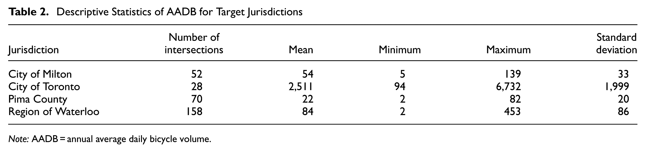
Note: AADB = annual average daily bicycle volume.
For Canadian jurisdictions, the 2016 census data was the source for demographic information and variables, and the 2022 census for Pima County, Arizona, US. To extract the explanatory variables provided in Table 1 for the target jurisdictions, open source data sets were obtained, including OpenStreetMap ( 23 ) data for network and land use variables in addition to open sources from target jurisdictions ( 24 – 28 ). The following section outlines the methodology used for estimating the AADB using the selected DD models, as well as the application and assessment of the chosen calibration models.
Methodology
Figure 1 shows the methodology for this study. First, the dependent variable from the selected DD models in the literature is examined. If the dependent variable is the AADB, the next step is to calculate the error metrics to assess the accuracy of the DD models as base models (naïve transferability). For dependent variables in other formats, such as 2-h PM counts, they need to be estimated as a form of AADB. The average ratio of the true AADB to the average 2-h PM counts is calculated for each site across all four target jurisdictions, then multiplied by the 2-h estimate from the DD models. Then, the error metrics must be calculated. In the next step, the selected calibration models from the literature ( 10 ) are applied using a Monte Carlo simulation. Finally, the error metrics are recalculated and compared with the base naïve transferability estimation of the AADB.
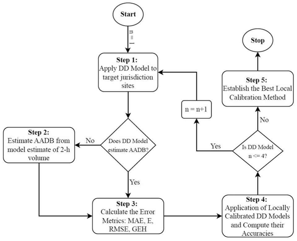
Methodology flowchart.
Step 1: Naïve Application of the DD Models
In the first step, all five DD models from Table 1 are applied to the four target jurisdictions to obtain estimates of bicycle volumes for all sites.
Two of the models (Strauss et al. [ 20 ] and Strauss and Moreno [21]) are structured to estimate bicycle volume as the AADB, so no further processing of these estimates is required. However, the remaining three DD models are structured to estimate exposure as bicycle volume in 2-h. For these three models, further processing, as part of Step 2, is required to estimate the AADB.
Step 2: Expansion of 2-h Volume Estimates to AADB
The two DD models developed by Tabeshian and Kattan ( 22 ) used data from Calgary, Canada, which included bicycle volume counts collected over 2 h from 04:00 to 06:00 p.m. across 34 sites. This paper reported a mean 2-h PM volume of 14.3 bicyclists but did not provide information on how this value can be scaled to estimate the AADB. To estimate the AADB, the average ratio of the AADB to the average 2-h bicycle PM volume for all sites across the four target jurisdictions was calculated, as shown by Equation 12. The average ratio was 7.26. This ratio was applied to each site’s 2-h volume estimate from the DD model to estimate the associated AADB.

where
The Griswold DD model ( 19 ) was developed using 2-h bicycle counts from 81 sites in Alameda County, California, US. The reported mean 2-h count was 35.8; however, these counts were recorded at various times of the day. The ratio of the 24-h volume to the 2-h volume for all 2-h periods in the day was computed using data from all sites in each jurisdiction. It was assumed that the counts were taken during the daytime, and the variation in the ratios for each 2-h period was examined. The ratio did not vary substantially between 08:00 a.m. and 06:00 p.m., and therefore the average ratio computed across these time periods (average ratio = 7.78) was used. This ratio was used to scale all the Griswold model estimates from 2-h volumes to the AADB.
Step 3: Compute the AADB Estimation Accuracy for Naïve Transferability of DD Models
In Step 3, the accuracies of the five DD models (listed in Table 1) applied to the four jurisdictions are quantified using the two error metrics adopted by (
10
) (

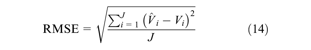
where
The GEH. performance metric, named after its creator, Geoffry E. Havers, considers the absolute difference and the percentage difference between the observed and estimated counts. It has been frequently used in applications, such as evaluating the adequacy of transportation simulation and urban transportation demand model estimates of link volumes. In these contexts, the desired threshold is that 85% of links have a GEH value ≤ 5.
Step 4: Compute the AADB Estimation Accuracy for Locally Calibrated DD Models
The five selected local calibration models ( 10 ) are described in the literature review section (Equations 2–6) and adapted for application to the five AADB DD models in Table 1. In the literature ( 10 ), the DD models were all log-linear models (i.e., the dependent variable is ln(AADPT), as in Equation 1). However, only four of the five AADB DD models in Table 1 are log-linear, and the remaining model (MLR model from Tabeshian and Kattan [22]) directly estimates bicycle exposure (the dependent variable is not ln-transformed). Therefore, the local calibration models were modified from Equations 2–6 to the non-log-transformed form of the AADB for application in the MLR model.
The local calibration models rely on the AADB values calculated from a set of sites in the local jurisdiction for which CCs are available. Consequently, the results are a function of the number of sites k in this set. Furthermore, the results will be impacted by which sites are in the local calibration set. Consequently, the evaluation method utilizes a Monte Carlo simulation process. For each replication, k random sites in the local jurisdiction are selected as local calibration sites for which the true AADB is known. The local calibration models (Equations 2–6) in combination with the five DD models are applied using this set of local calibration data to produce estimates of the AADB for each site in each jurisdiction. For each value of k, 300 replications of the Monte Carlo simulation were performed. The value of
In practical applications, despite the methods used for estimating AADBs, such as expansion factors with short-term and CCs or DD models, unrealistic estimates (i.e., significant over- or underestimations) may occur. A practical approach for identifying and controlling these extreme errors is to establish and apply upper and lower thresholds to the estimation result, and this approach is adopted in this step. The lower threshold is 0.001 across all jurisdictions, as the AADB must be non-negative, and values of zero result in divide-by-zero errors from some local calibration models. In practice, the selection of an upper threshold would be informed by local knowledge of the level of bicycle activity in the target jurisdiction. Consequently, the following upper thresholds on the AADB estimates were applied: (1) City of Toronto = 10,000; (2) City of Milton = 1,000; (3) City of Waterloo = 1,000; and (4) Pima County = 500. If a model estimate of the AADB exceeded the upper threshold, it was replaced with the upper threshold; if it was less than the lower threshold, it was replaced with the lower threshold. The maximum threshold values were selected to exceed the maximum observed AADB for each jurisdiction (Table 2) to not artificially improve prediction accuracies by selecting threshold values equal to the maximum observed AADB values.
The mean and median of each of the four error metrics from the 300 replications were recorded for each combination of the DD model, local calibration model, jurisdiction, and k.
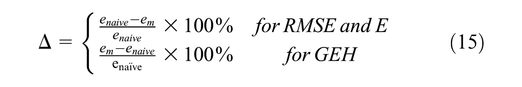
Step 5: Establish the Best Local Calibration Method and Quantify the Associated Performance Improvement
The last step of the assessment methodology is to compare the AADB estimation accuracy of the DD models without local calibration (i.e., naïve transferability) and with local calibration. This is achieved by computing the percentage improvement in the error metrics, as shown in Equation 15. Note that for the error metrics
where
The next section presents and discusses the results.
Results and Discussion
This section of the paper is organized into three subsections, providing results from methodology Steps 2, 4, and 5, respectively.
Naïve Transferability of DD Models (Step 2 Results)
Table 3 provides the performance metrics for each DD model applied to each target jurisdiction. These results indicate that the spatial transferability performance of the five DD models varies widely across the four target jurisdictions and that the spatial transferability performance is quite poor. The average MAE. (Equation 7) is 623.9, with a minimum of 128.2 for Pima County and a maximum of 2,069.2 for the City of Toronto. The average error (Equation 8)
Performance Summary of Naïve Transferability of DD Models Applied to Target Jurisdictions
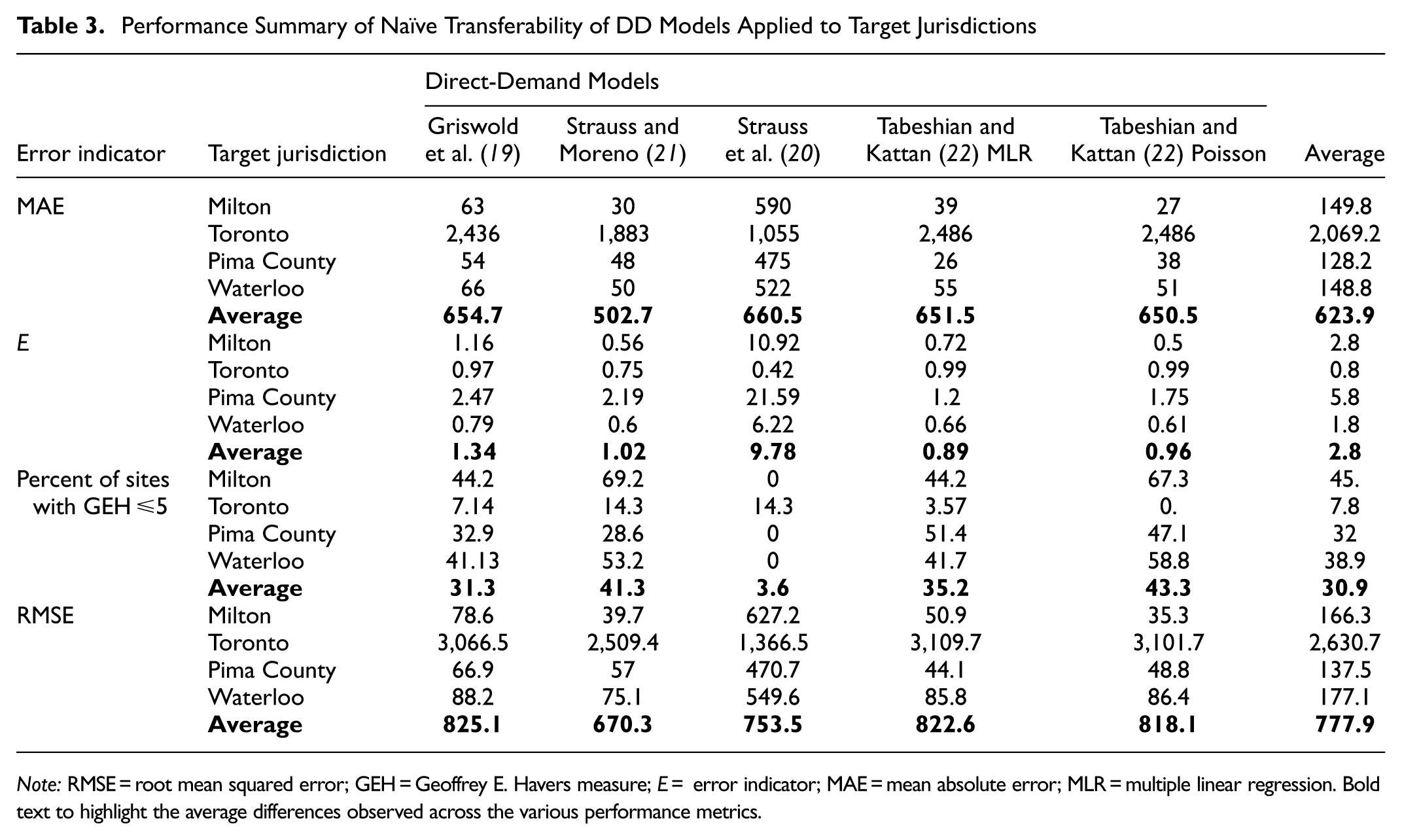
Note: RMSE = root mean squared error; GEH = Geoffrey E. Havers measure; E = error indicator; MAE = mean absolute error; MLR = multiple linear regression. Bold text to highlight the average differences observed across the various performance metrics.
Compute the AADB Estimation Accuracy for Locally Calibrated DD Models (Step 4 Results)
The substantial estimation errors observed in the naïve transferability results highlight the need for better approaches to adapt DD models in a local jurisdiction. Figure 2 shows the effectiveness of the local calibration models for improving the accuracy of the DD models. For each graph, the y-axis represents the mean error indicator
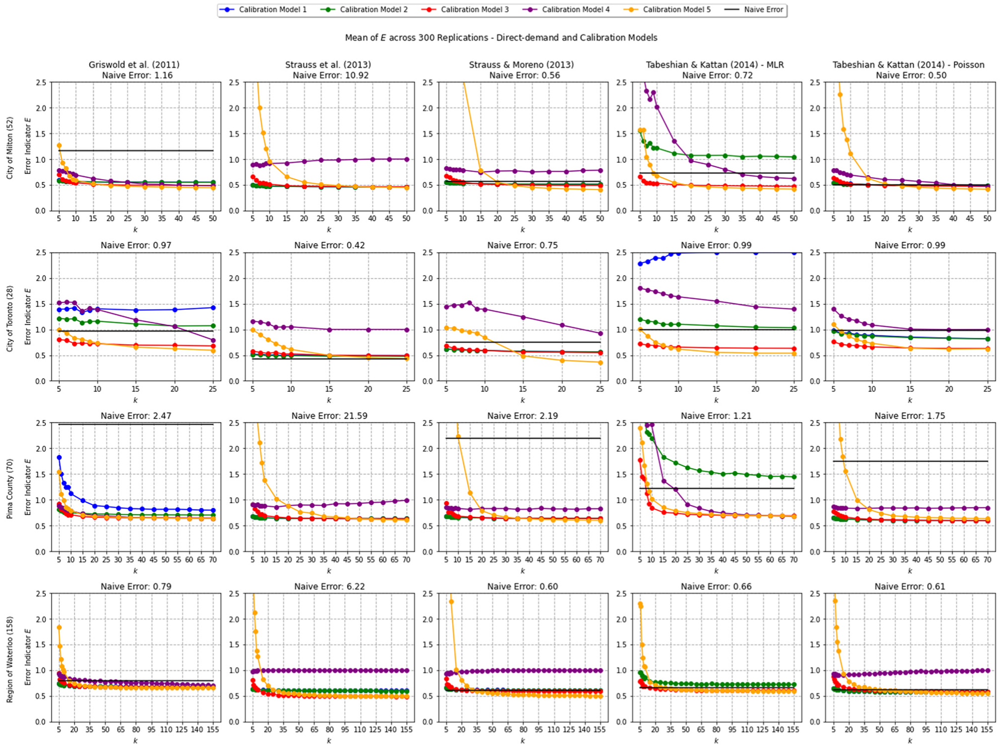
Performance of each direct-demand (DD)model (mean E over 300 replications) as a function of target jurisdiction, local calibration method, and number of local calibration sites (y-axis limited to 2.5).
Several observations can be made from the results shown in Figure 2.
In almost all cases, locally calibrating a DD model substantially improves the accuracy of the estimated AADB values.
The amount of improvement varies by local calibration model and by target jurisdiction.
There are some cases (especially for lower values of
Local calibration Models 2, 3, and 5 appear to perform much better than local calibration Models 1 and 4.
The performance of some of the local calibration models (particularly Model 5) is highly sensitive to the number of sites
Establish the Best Local Calibration Method and Quantify the Associated Performance Improvement (Step 5 Results)
Because the results from Step 4 demonstrated notable accuracy improvements, the next step was to identify which calibration model performs best and to quantify the magnitude of improvements. Figure 3 shows the overall performance of the local calibration models across all DD models, based on the mean and median values of the error indicator
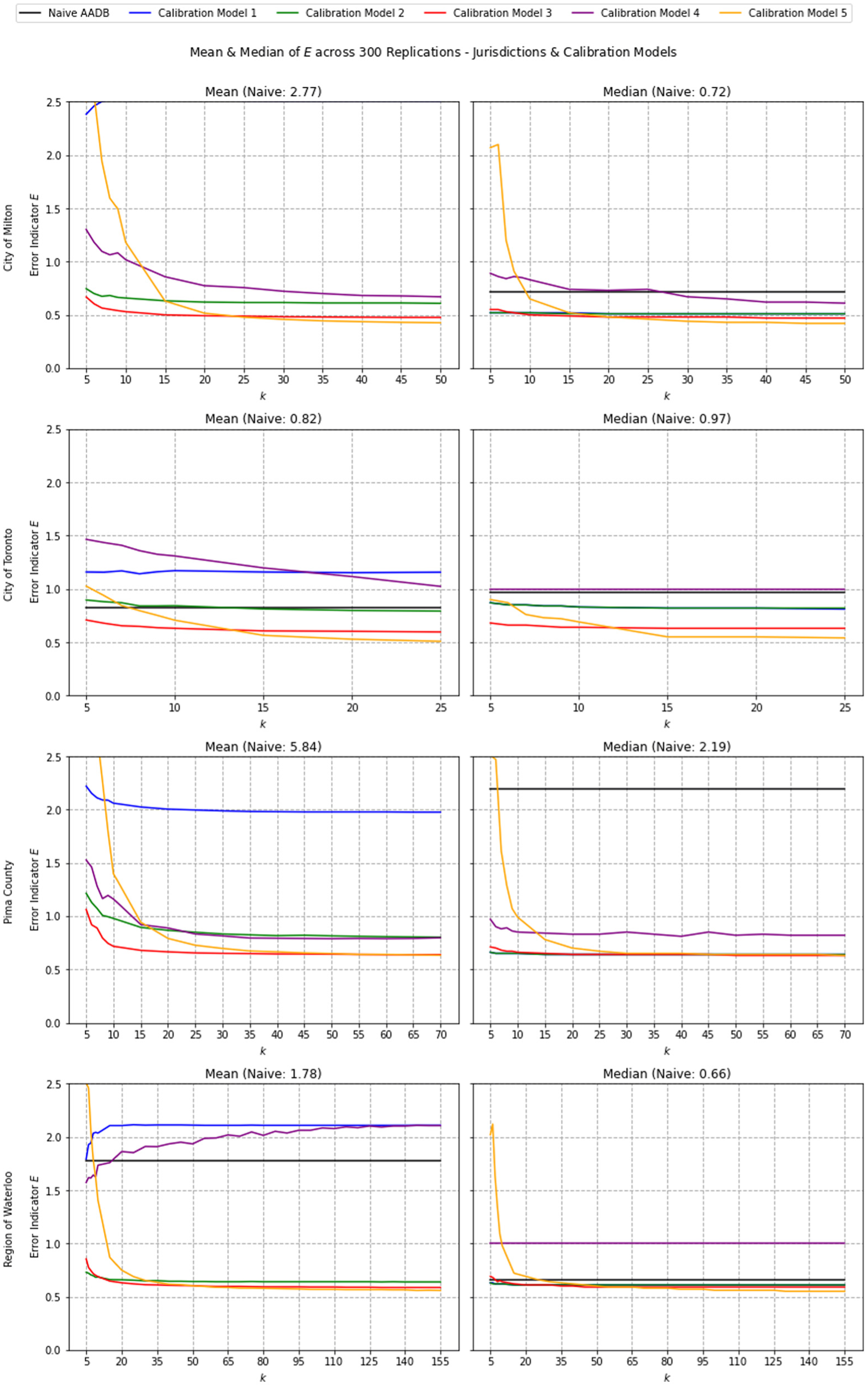
Performance of all direct-demand (DD) models (mean and median of E over 300 replications) as a function of target jurisdiction, local calibration method, and number of local calibration sites (y-axis limited to 2.5).
Calibration Model 3 provides lower mean values of the error indicator
All performance comparison results for calibration methods are based on 300 replications. In practice, a jurisdiction will only apply the local calibration model once using the data from available sites. Therefore, the mean or median of a larger number of replications may not be meaningful. Instead, another analysis was conducted to determine the average probability of achieving a lower error indicator
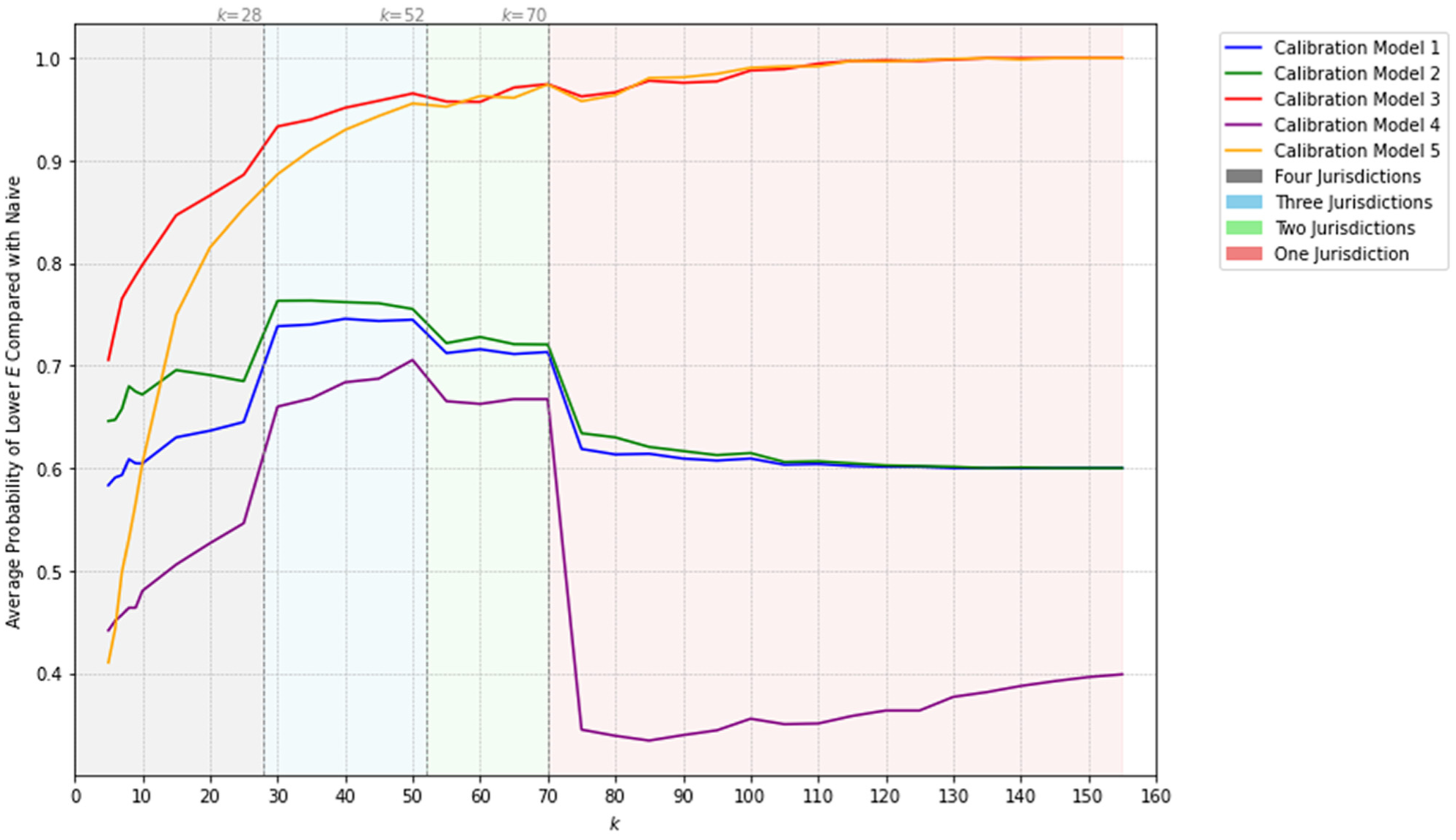
Average probability over 300 replications that local calibration provides a lower error
In Step 5 of the methodology, the percentage improvement in error metrics (Equation 15) was calculated. Figure 5 shows the percent improvement in the error indicator
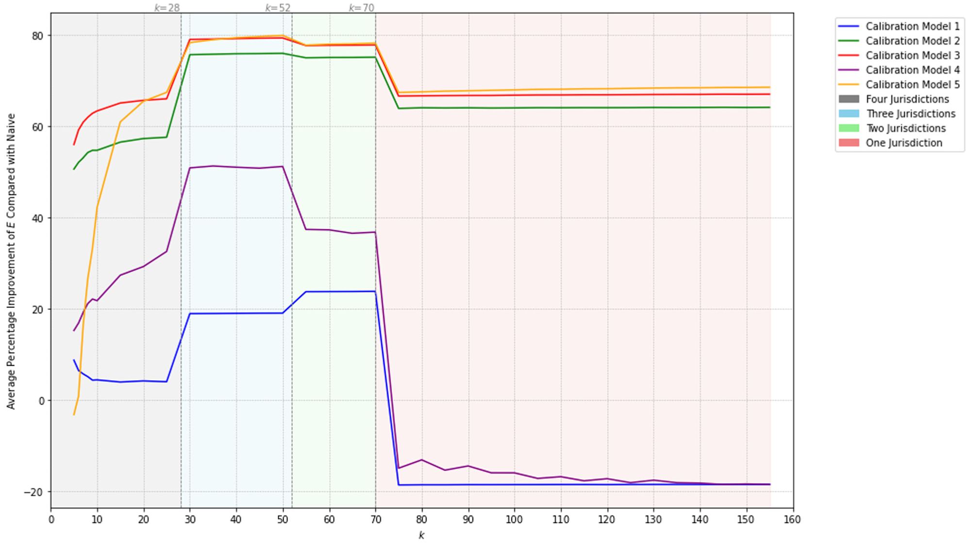
Percentage improvement (
Even for a small value for
Figure 5 shows the performance improvement obtained from the use of local calibration models when only considering the error metric
Figure 6 shows the optimal local calibration model (i.e., the model that provides the largest average performance improvement Δ across the four jurisdictions versus the naïve application of the DD models) for each value of
Despite the error metric considered, local calibration Models 3 and 5 perform better than Models 1, 2, and 4 because these three models are never the best models for any error metric or value of
The results show that Model 5 is best according to all four performance metrics for
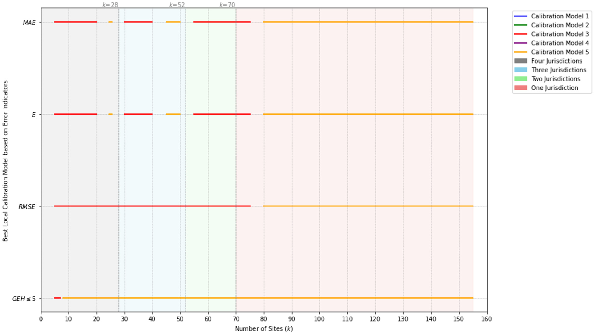
Best local calibration model for each error metric as a function of
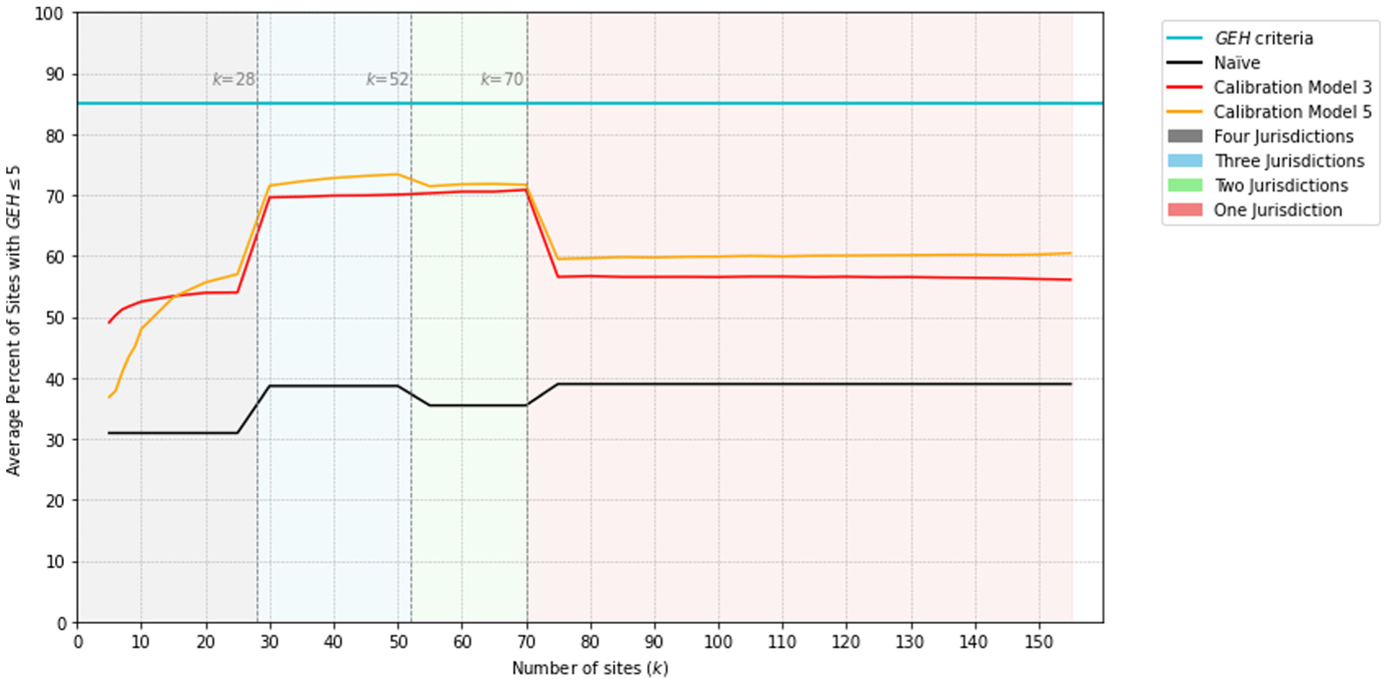
Average percentage of sites with GEH ≤ 5 as a function of
Conclusions
This paper examines whether calibration methods can enhance the naïve transferability of existing DD models for AADB estimation. Drawing on calibration methods from a similar study on pedestrians, these techniques were applied across four target jurisdictions, covering 308 sites: (1) City of Toronto (28); (2) City of Milton (52); (3) Region of Waterloo (158); and (4) Pima County (70). Five existing DD models were the base for naïve transferability and subsequent calibration tests. Following an initial examination of naïve transferability, two threshold filters were introduced to address extreme overestimations and underestimations in the AADB estimation. The lower threshold was set at 0.001 across all four target jurisdictions, and the upper threshold varied depending on the jurisdictions. The findings demonstrate that these thresholds, particularly for lower site counts (i.e.,
The results of this paper suggest that calibration, particularly regression-based methods, provides a substantial improvement in the accuracy of AADB estimates derived from spatially transferred DD models. Across all four target jurisdictions, Calibration Model 3 consistently outperformed others for lower site counts k, providing a 56% reduction in the error indicator
The main finding of this paper is that locally calibrating DD models substantially improves the accuracy of AADB estimates from spatially transferred DD models. This finding is supported by investigating different error indicators over a variety of sites that might be available for location calibration within a jurisdiction. Considering the ease of use and practicality of the calibration models, all five have a similar level of technical complexity. However, they may differ in ease of application. Models 1 and 2 can be viewed as scaled-based models that are slightly easier to apply and may not require highly technical skills. However, as the results show, they may not be the most effective for improving naïve transferability. Models 3 and 4 are slightly more technical but still relatively straightforward to use because they are based on linear and power regression, respectively. Like Models 1 and 2, they only require the naïve estimates and observed AADB as inputs. Among all five, Model 5 may be the most advanced for input requirements, as each coefficient is calibrated separately. However, for ease of use, it remains quite practical and comparable with the other models, as supported by the results. It is recommended that local calibration Model 3 is used when the number of sites in the local jurisdiction with available AADB counts is less than 80. When counts are available for 80 or more sites, then local calibration Model 5 should be used. When AADB counts are available for many sites in the target jurisdiction, it may be more appropriate to develop a DD model for the target jurisdiction rather than locally calibrate a DD model originally developed in another jurisdiction. The number of sites
In this paper, the effectiveness of regression-based local calibration models was explored. Future research should explore other forms of local calibration, such as machine learning techniques, Bayesian calibration, or both.
Practical Implications
Developing DD models can be challenging for jurisdictions that lack sufficient CC sites, resources, comprehensive data collection from multiple sources, and technical expertise. Therefore, this paper demonstrates that using and adapting existing DD models can effectively address data and resource limitations faced by jurisdictions. This paper also shows that implementing practical calibration models that are technically straightforward and easy to use can be a cost-effective approach for jurisdictions to estimate bicycle volumes at intersections.
Supplemental Material
sj-docx-1-trr-10.1177_03611981251401589 – Supplemental material for Improving the Accuracy of the Spatial Transferability of Direct-demand Models for Bicycle Volume Estimation at Intersections
Supplemental material, sj-docx-1-trr-10.1177_03611981251401589 for Improving the Accuracy of the Spatial Transferability of Direct-demand Models for Bicycle Volume Estimation at Intersections by Sina Azizi Soldouz and Bruce Hellinga in Transportation Research Record
Footnotes
Acknowledgements
The authors gratefully acknowledge the Region of Waterloo, City of Toronto, City of Milton, and Pima County for providing permission to use the bicycle count data and for providing rich open data portals that were essential sources of information for this research, and Miovision for providing access to the bicycle data. The work in this paper reflects the views of the authors and there is no explicit or implicit endorsement by any of the aforementioned jurisdictions or companies.
Author Contributions
The authors confirm contribution to the paper as follows: study conception and design: Hellinga, Azizi Soldouz; data collection: Azizi Soldouz; analysis and interpretation of results: Azizi Soldouz, Hellinga; manuscript preparation: Azizi Soldouz, Hellinga. All authors reviewed the results and approved the final version of the manuscript.
Declaration of Conflicting Interests
The authors declared no potential conflicts of interest with respect to the research, authorship, and/or publication of this article.
Funding
The authors disclosed receipt of the following financial support for the research, authorship, and/or publication of this article: The authors gratefully acknowledge financial support from the Natural Sciences and Engineering Research Council of Canada and Transport Canada. The research was carried out by the authors, and no endorsement of the methods or findings by funding agencies is claimed or implied.
References
Supplementary Material
Please find the following supplemental material available below.
For Open Access articles published under a Creative Commons License, all supplemental material carries the same license as the article it is associated with.
For non-Open Access articles published, all supplemental material carries a non-exclusive license, and permission requests for re-use of supplemental material or any part of supplemental material shall be sent directly to the copyright owner as specified in the copyright notice associated with the article.