
Abstract
Bicycle volume estimation is essential for effective city planning and ensuring the safety of vulnerable road users. Traditional approaches often involve resource-intensive data collection, such as short-term counts expanded using continuous counts (CCs), or the development of direct-demand models from site-specific data such as geometry, socioeconomic, and land use. Although recent efforts have explored crowdsourced data, such sources may be biased and not consistently available across jurisdictions. This study explores the potential of large language models (LLMs), specifically ChatGPT-4o mini, as a low-cost and accessible alternative for estimating bicycle volume levels at intersections.
A data set of CCs over 12 months and site characteristics for 158 signalized intersections in the Region of Waterloo, Ontario, Canada, was compiled. From this, the average annual daily bicycle volume was computed, and intersections were categorized into low, medium, or high volume levels.
Eight LLMs and three benchmark approaches, including a Naïve (random), an ordered logit (OL) model, and human survey responses, were applied to the data set. Accuracy in predicting the correct volume category was the evaluation metric. The best-performing LLM requires only two input features: (1) bike lane length (km); and (2) the presence of schools, and achieves an average accuracy of 60%, just 4% below the OL model, and significantly better than the Naïve model and human survey respondents. Of interest, providing satellite images or additional quantitative input variables decreased the LLM performance. The results suggest LLMs can offer a scalable, data-efficient alternative for jurisdictions lacking extensive bicycle count data or modeling expertise.
Keywords
Introduction
Volume (also referred to as exposure) is a key input to road safety analysis and for planning transportation infrastructure requirements and improvements. Traditionally, focus has been on vehicular traffic and is frequently expressed as the annual average daily traffic (AADT). However, with the growing focus on improving the safety of vulnerable road users, such as bicyclists and pedestrians, estimating their exposure has become equally important. Analogous exposure measures for pedestrians and bicyclists are annual average daily pedestrian traffic and annual average daily bicycle (AADB) volume, respectively.
Several methods have been used to estimate bicycle volumes. The most common is to use factoring methods to scale up short-term counts (STCs) to estimate a longer-term average volume (e.g., AADB). The scaling factors capture temporal variations (by time of day, day of the week, and month of the year) and are typically computed from a smaller number of locations at which continuous counts (CCs) are available. These factoring methods work well, but STCs must be available for all sites of interest, and scaling factors must be available (or be computed from data from CC sites).
When jurisdictions do not have (sufficient) STCs and/or CCs, then statistical methods, such as direct-demand (DD) models, have been used. The DD models typically associate bicycle volumes (e.g., AADB) with socioeconomic and land use characteristics of the area directly surrounding the site of interest. The main challenge with DD models is that a large data set with known bicycle volumes is required to develop the DD model.
More recently, methods utilizing crowdsourced data, such as Strava ( 1 ) and StreetLight ( 2 ) data, have gained popularity. Crowdsourced data from dedicated platforms such as Strava provides detailed trajectory data from individual trips. However, there are challenges with sampling bias (not all bicyclists use these apps), and the sampling rate is unknown and varies temporally and spatially. Other sources of crowdsourced data face these and other challenges, such as correctly distinguishing between different modes (e.g., pedestrian versus bicyclist). Despite the range of methods that have been and are being used in practice, a need for an accurate, cost-effective, and robust method for estimating bicycle volumes remains.
Machine learning (ML) approaches such as random forest (RF), eXtreme Gradient Boosting (XGBoost), and deep neural network methods have been applied to the problem of estimating pedestrian and bicyclist volumes ( 3 ). These ML techniques have advantages over traditional statistical models, including improved ability to capture nonlinearities, no need to specify the functional form of the relationship, and fewer assumptions about the underlying distributions of errors. However, these methods have limitations, including the need for relatively large training data sets, the possibility of large computational loads for training, and the propensity for overfitting when training data sets are not sufficiently large.
There have been tremendous advances recently in artificial intelligence (AI) and, in particular, large language models (LLMs). The LLMs have been applied to a wide range of transportation problems, including:
Various applications in intelligent transportation ( 4 );
Investigating LLMs’ risk perceptions from forward-facing traffic images ( 5 );
Bridging the gap between machine execution and human intention in human–machine interactions using LLMs as a “co-pilot” ( 6 );
Utilizing prompt engineering and LLMs to interact with traffic data imputation systems, enabling users to request information using simple language without needing knowledge of the detailed information or mathematical modeling behind it ( 7 );
Exploring the combination of LLMs and vision-language models to evaluate image-based questions from driving license tests, such as traffic sign image questions, scenario-based questions with images, and a combination of both ( 8 );
Using natural language processing and advanced language models to classify pedestrians’ maneuvers before a crash based on crash data and police reports ( 9 ).
The LLMs are particularly well-suited to handle unstructured data and address complex and nonlinear relationships. They are widely available at low cost and do not require expertise in statistical model fitting to apply. Furthermore, general LLMs, such as ChatGPT, are not trained on a data set from a specific jurisdiction. This is particularly important because it means that there is no need to have a training data set of known AADBs from the local jurisdiction to apply the model.
This leads to the main research question for this study: Can LLMs be used to estimate bicycle volumes with sufficient accuracy to be of practical value? In addition, this study determines how the LLM estimation accuracy is affected by the prompt and input information. The analysis is carried out using bicycle volume counts collected at a set of 158 signalized intersections in the Region of Waterloo, Ontario, Canada, over 12 months.
The remainder of this study is organized as follows. The next section presents a review of the literature, including benchmark models in bicycle volume estimation, as well as relevant studies investigating volume assessments using LLM models. Then, the data used in this study is described, followed by the Methodology, Results, and Conclusion sections. Finally, limitations of this study are discussed.
Literature Review
A large body of literature exists on methods for estimating bicycle volumes. Existing methods can generally be classified into six categories.
Direct calculation in which long-term volumes (typically AADB) are calculated directly from counts from CC sites ( 10 ). Because these methods can only be applied to CC locations and most jurisdictions have a small fraction of their intersections instrumented with CC technologies, the application domain of these methods is limited.
Expansion methods in which STCs are expanded into long-term volumes (typically AADB) using expansion factors calculated from CC sites ( 11 – 13 ). The expansion factors reflect temporal variations in bicycle activity (across days of the week and seasonality). Therefore, these temporal patterns must be identified, the available CC sites must be grouped into temporal patterns (factor groups), and then expansion factors must be computed for each temporal pattern (factor group). Finally, a temporal pattern (and the associated set of expansion factors) must be associated with each STC site. Much research has been performed to: (1) propose methods for defining temporal patterns; (2) recommend a minimum number of CC sites for each factor group; and (3) quantify the effect that duration (e.g., 1, 2, … 7 days) of the STC has on the AADB estimation accuracy.
DD models are statistical models in which the long-term bicycle volume (dependent variable) is estimated as a function of the set of explanatory variables that reflect land use, demographics, and transportation infrastructure characteristics ( 14 – 20 ). The main challenge with DD models is that a relatively large data set of known volumes is required to develop the model. Studies have also explored the spatial transferability of DD models for pedestrians ( 14 ) and bicyclists ( 15 ). However, applying these models naively has led to significant estimation errors. These errors, quantified as the average absolute error between the estimated and actual counts across all sites in a jurisdiction, divided by the average actual count, are from 0.52 to 50 for pedestrian volume ( 14 ) and 0.41 to 31.9 for bicyclist volume ( 15 ).
Network models include travel demand models (TDMs) and other models that incorporate some form of bike trip origin–destination (O–D) demand matrix (or matrices) and then assign these trips to the network via a route assignment algorithm. The advantage of these models is that they can provide estimates for all locations in the network, not just intersections; however, general TDMs are typically used to assess large-scale land use and transportation network decisions over long time horizons. Aggregate four-step TDMs typically have poor accuracy for estimating bicyclist volumes. These models divide the network into traffic analysis zones that typically do not provide the spatial resolution appropriate for bike trips, which are shorter than motorized vehicle trips ( 21 ). Activity-based TDMs are disaggregated but require greater input data and are less frequently used by jurisdictions. Dedicated bike network models can have higher accuracy but typically require a bike trip O–D matrix as an input and a calibrated bike trip assignment model; information that jurisdictions frequently do not have. For example, Bhowmick et al. ( 22 ) developed a bike volume estimation model using 4 years of an activity survey to derive origins and destinations and used GPS trace data from almost 20,000 cycling trips to develop a route choice model. They reported a mean absolute percent error = 25% for bike volume counts across 48 links in Melbourne, Australia.
Crowdsourcing, in which a sample of bicycle trips is observed. These observations are typically over a much longer period of time than STCs, and often include the entire trajectory of the trip, but represent only a sample of all bicycle trips made during the observation period. Then, techniques are applied to expand the sample to obtain an estimate of the total number of trips ( 2 , 23 , 24 ).
Hybrid methods, which are a combination of Methods 1–5. Typically, these hybrid methods are a combination of crowd-sourced data and expansion methods, or the use of ML and deep learning approaches ( 3 , 16 , 23 , 25 , 26 ).
Each of the previous categories of methods has unique strengths and limitations. The most significant constraint for most jurisdictions is the lack of data (bike trip O–D matrix, sample of bike trip trajectories, CCs, and/or STCs), which precludes the application of the previous methods.
Recent advances in AI models, including LLMs, and the ease of accessibility to these models present them as a potentially effective and efficient method for estimating bicycle volumes at intersections. However, no previous studies could be found that applied LLMs to the problem of estimating bicycle volumes at intersections. However, LLMs have been applied to other similar transportation applications.
Driessen et al. ( 5 ) evaluated ChatGPT-4 Vision’s (GPT-4V) ability to estimate risk levels from forward-facing road traffic images and compared its performance with human responses. Performance was measured by calculating the correlation coefficient between AI-generated risk scores and human assessments across 210 images. The results showed a correlation coefficient of 0.79, demonstrating a high degree of correlation between the AI rankings and human assessments.
Li et al. ( 27 ) applied and evaluated several LLMs, including one that included a spatio-temporal encoder to capture temporal dependencies, to predict bicycle inflows to and outflows from 80 regions (approximately 1 × 1 km) within New York City (NYC). They used NYC-bike data sets from the first 2 weeks of January 2020. For a given region, they provided land use information and the historical inflows and outflows for the 12 30-min periods from noon to 06:00 p.m. and then directed the LLM to predict the inflows and outflows for the next 12 30-min periods (i.e., 06:00 p.m. to midnight). They found that the LLM generally performed well, but the model with the spatio-temporal encoder performed best because this model could capture the temporal dependencies between the 30-min intervals.
Other studies have evaluated the performance of LLMs to: (1) correctly answer driving license test questions ( 8 ); (2) determine pedestrians’ maneuvers before a crash ( 9 ); and (3) predict pedestrian crossing behavior at crosswalks ( 28 ).
In a study focused on estimating pedestrian volumes at intersections, Sobreira and Hellinga ( 29 ) investigated the use of ChatGPT-4V to rank urban intersections based on the level of pedestrian activity when the LLM was only given satellite images of the area directly surrounding the intersections. The results revealed a strong correlation (0.73) between the true rankings and those estimated by ChatGPT-4V. In addition, a novel methodology was proposed and tested, which combined a sample of intersections with known pedestrian volumes and ChatGPT’s rankings to estimate pedestrian volumes at other ranked sites. The study found that ChatGPT could rival and, in some cases, outperform traditional methods such as DD models. This highlights the potential of ChatGPT for estimating bicycle volumes, offering a simpler alternative to traditional statistical and factoring methods.
To the best of the authors’ knowledge, no other studies evaluate the potential usage of LLMs for estimating long-term bicycle volumes at intersections. This study aims to assess the accuracy of LLMs in estimating bicycle volumes (AADB) at intersections using different scenarios as inputs and examines their practicality compared with the existing benchmark models.
Data Description
A total of 256 signalized intersections were selected as target locations in the Region of Waterloo, Ontario, Canada, as a permanently deployed camera-based CC data collection system provided by a single vendor existed at these locations. These counts included minute-by-minute bicycle data for each turning movement and crossing at the intersections. Counts per minute were aggregated to form counts for each calendar day (i.e., 24-h). Count data were acquired from these sites with the objective of obtaining data from a full year, from July 1, 2023, to June 30, 2024. At some of the intersections, the data collection system had not been deployed for the full year period; 170 intersections met the 1-year data availability condition.
The camera-based count system only reports counts when one or more entities (vehicles, pedestrians, or bicyclists) are detected in a 1-min interval. Consequently, the system does not distinguish between periods with no activity (zero counts) and periods when there is an issue with the system (e.g., power loss) and no counts are recorded. Therefore, in this study, a 24-h count is considered valid if there was at least one vehicle, pedestrian, or bicyclist detected in the 24-h period. Sites were included in this study only if the camera-based system was installed for 12 months, and there were no significant data gaps (sites were excluded if no vehicle traffic was detected for more than 4 consecutive days). After applying the above filtering process, 158 sites remained, and these sites formed the data set used in this study.
The true AADB was computed from the observed counts using Equation 1.

where
Methodology
The goal of this study is to quantify the performance of an LLM using GPT-4o mini, to estimate the AADB category (low, medium, and high as defined in the Data Description section) of a set of sites and to compare this performance with benchmark methods. The methodology of this study is structured into six phases, as shown in Figure 1. Each of these phases is described in the following subsections.
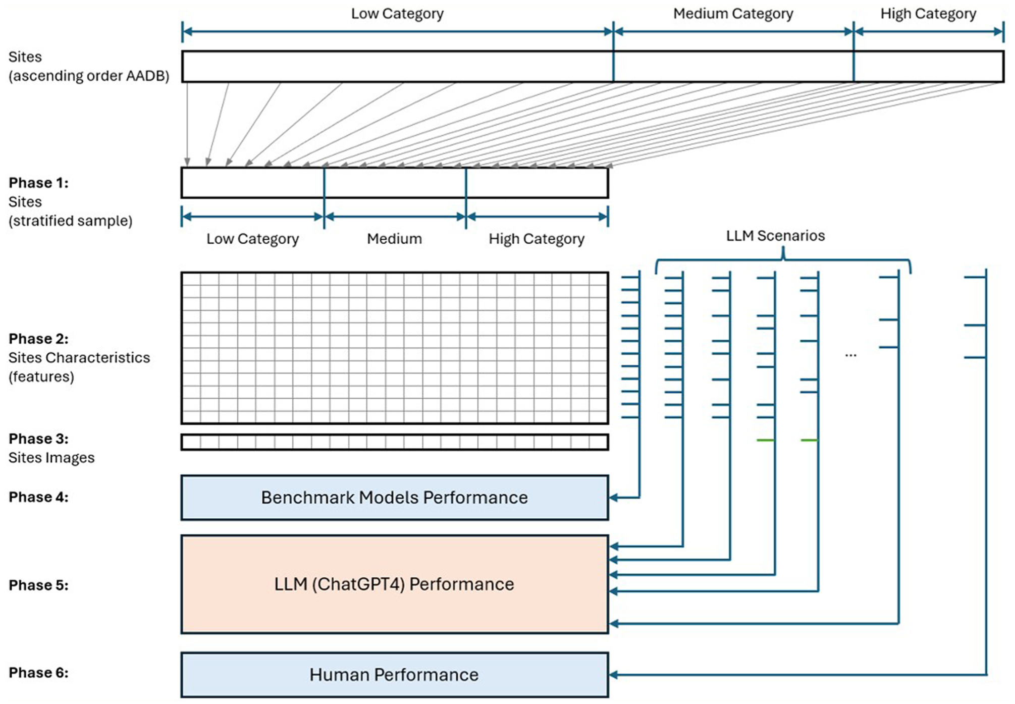
Methodology framework.
Phase 1: Site Selection
The level of bicycling activity at intersections varied considerably across the different CC sites. Based on the frequency distribution of the AADB, three levels (categories) of cycling activity were defined: low, medium, and high, as shown in Figure 2. The boundaries for these categories were established as follows: low = AADB ≤ 50; medium = 50 < AADB ≤ 150; and high = AADB > 150 bicycle counts per day. Within these categories, 75 sites were identified as low, 57 as medium, and 26 as high. To ensure equal representation across the three AADB categories, 75 sites (25 per category) were selected using stratified random sampling.
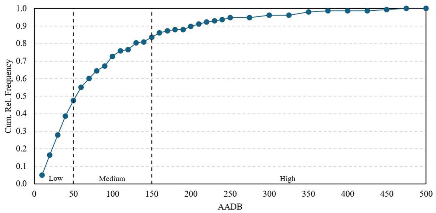
Cumulative relative frequency (Cum. Rel. Frequency) distribution of AADB for 158 study sites.
Phase 2: Site Features
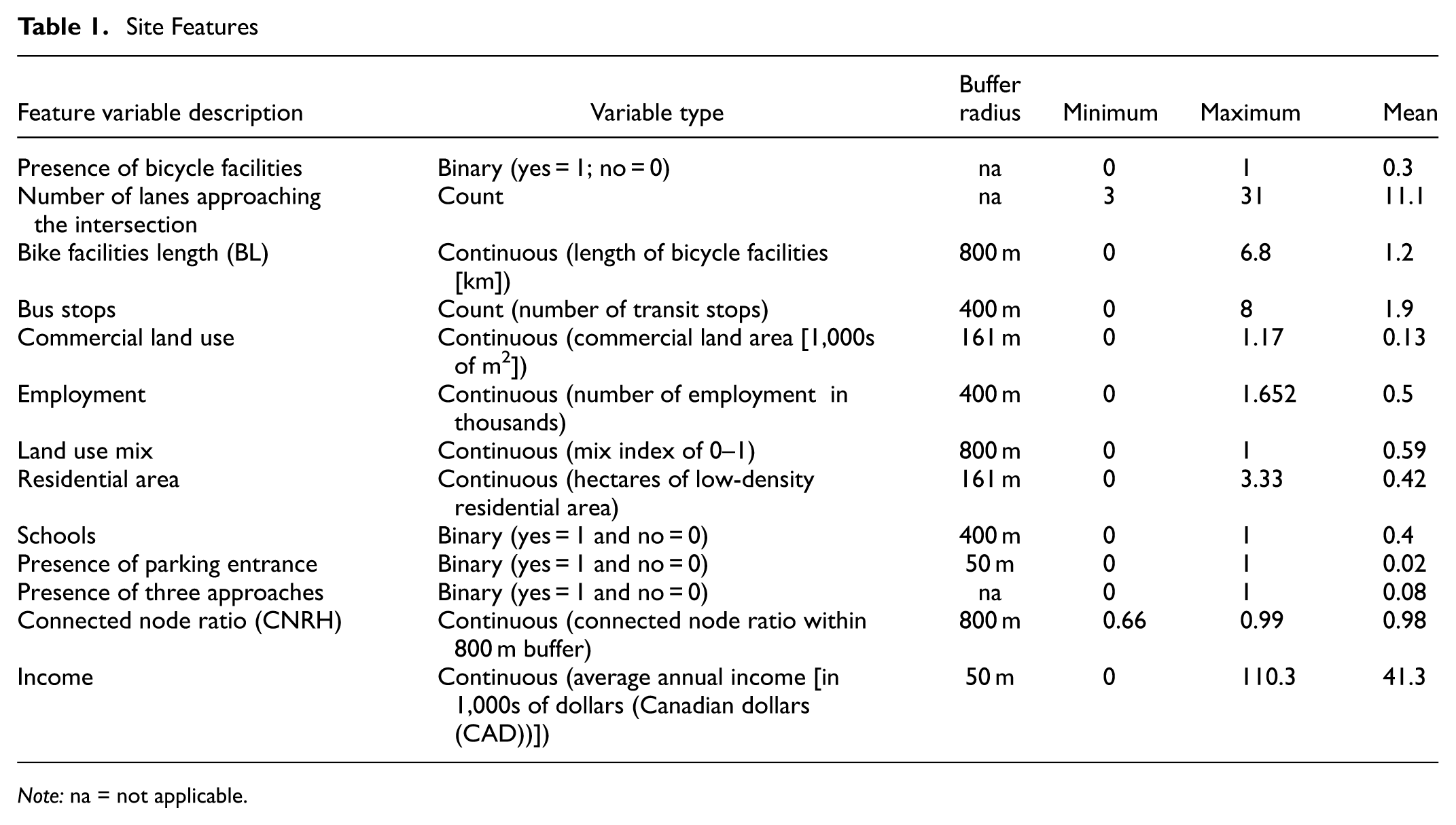
Demographic information and variables were sourced from the 2016 census data. To derive the explanatory variables listed in Table 1, open-source data sets were utilized, including OpenStreetMap ( 30 ) for network and land use variables, along with additional open data from the City of Waterloo ( 31 ). These characteristics were selected based on the shortlisted DD models from a study conducted by Azizi Soldouz and Hellinga ( 15 ). Their study examined the spatial transferability of existing DD models in estimating the AADB for a different jurisdiction. The shortlisted models were chosen based on the retrievability of their variables for other jurisdictions. Similarly, in this study, features from these DD models were selected based on two criteria:
Characteristics that are most commonly used in DD models;
Characteristics that are quantitative and easier for jurisdictions to extract.
Site Features
Note: na = not applicable.
Phase 3: Site Satellite Images
In Phase 3, satellite images of all selected sites were extracted using the Google Cloud Platform ( 32 ). These images were utilized either as a stand-alone scenario or in combination with quantitative features for the category estimation process. The images were square-shaped, centered on the coordinates of each intersection, with an area coverage of approximately 70 × 70 m per image. This zoom level effectively captures the geometry of the intersections, such as the number of lanes and the presence of bike lanes. An example of the satellite image used with OpenAI Application Programming Interface (API) models is shown in Figure 3.
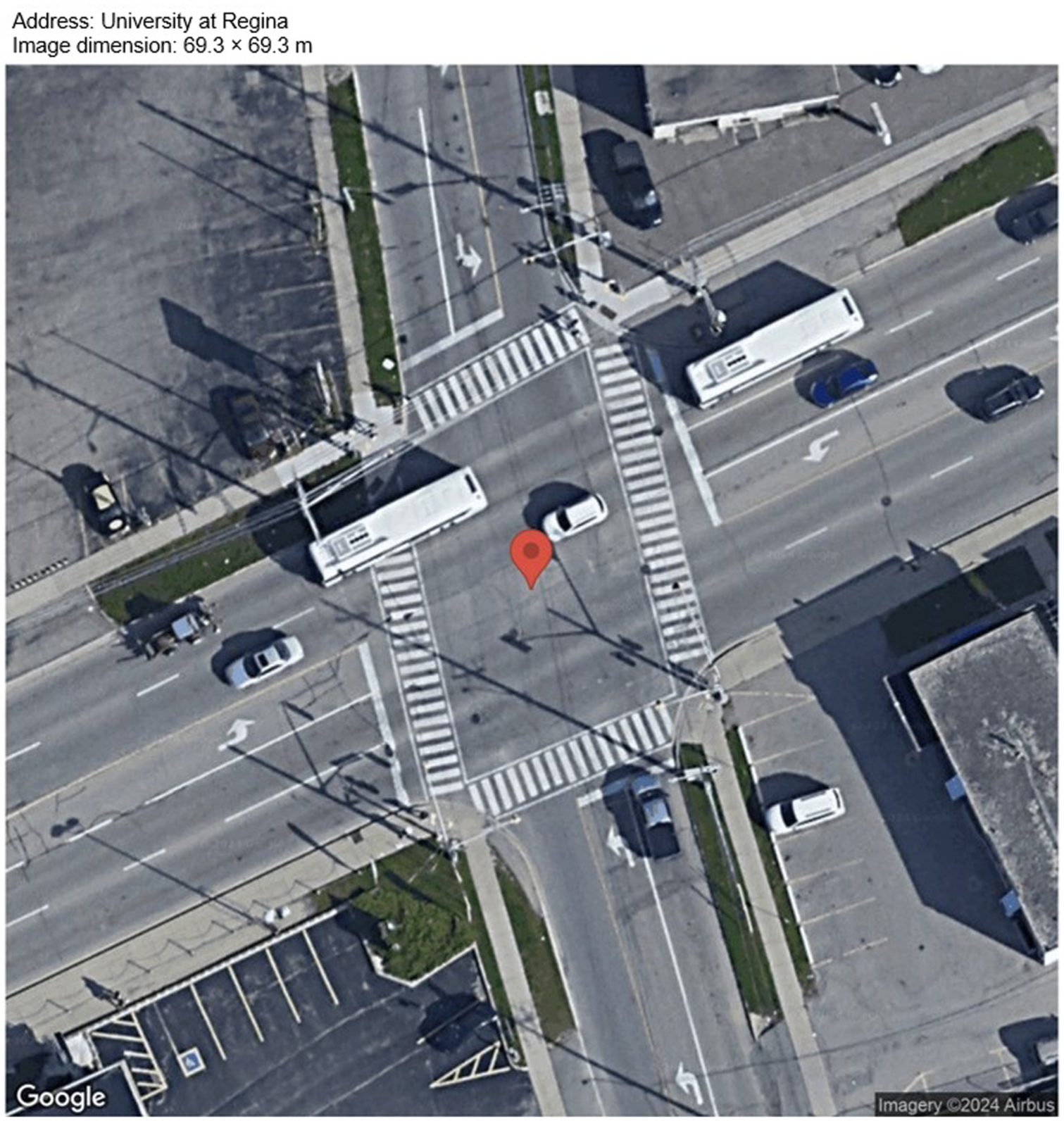
Example of satellite image ( 33 ) used for LLMs examination.
Phase 4: Benchmark Models
Given the novelty of LLMs, particularly in addressing transportation engineering problems, it is crucial to conduct a comprehensive analysis using benchmark models for comparison. Therefore, two benchmark models were developed.
The first benchmark model (BM1) is a Naïve model, which randomly assigns one of three categories (low, medium, or high) to each of the 75 selected sites without considering any associated site characteristics. The BM1 is applied 30 times to each site to create 30 replications.
The second benchmark model (BM2) is an OL model, which estimates the AADB category for each site from the site characteristics. To develop the best OL model, the underlying latent variable

where
The site features from Table 1 were considered as explanatory variables in the logit model. Explanatory variables most strongly correlated with the dependent variable were selected, while accounting for multicollinearity among the independent variables using the variance inflation factor (VIF < 5). A stepwise regression method was employed to determine the optimal OL model, maximizing the accuracy of category prediction and minimizing the Akaike Information Criterion (AIC).
The observed categories


The performance of all models, including the benchmark models, was expressed in a confusion matrix (Table 2) and summarized by computing the categorization accuracy using Equation 2.
Confusion Matrix: Accuracy Calculation
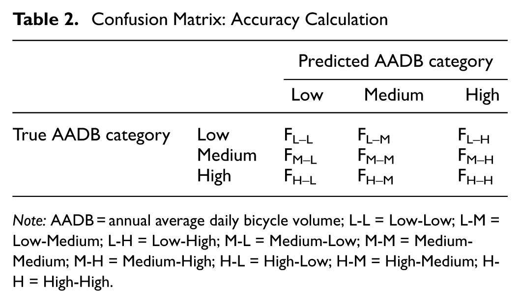
Note: AADB = annual average daily bicycle volume; L-L = Low-Low; L-M = Low-Medium; L-H = Low-High; M-L = Medium-Low; M-M = Medium-Medium; M-H = Medium-High; H-L = High-Low; H-M = High-Medium; H-H = High-High.
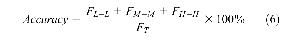
where
F x–y = number of sites that are in AADB category x and predicted to be in AADB category y, and
F T = sum of F x–y for all AADB categories (F T = 75 in this study).
These benchmarks serve as a baseline for comparing the accuracy of their predictions against those generated by the OpenAI API. The performance of all models was compared using confusion matrices and accuracy in predicting the correct category for the selected 75 sites, averaged over 30 replications for the LLMs and Naïve models.
Phase 5: LLMs
The performance of an LLM is expected to be influenced by the information provided to the LLM as part of the prompt. Consequently, different LLM scenarios were created, each with different prompt information. The performance of the LLM for each scenario was quantified using the same metrics (i.e., confusion matrix and accuracy) as described in Phase 4 and used for the benchmark models.
Scenarios were developed to answer the following five key research questions.
All LLM prompts with variables started with the following phrase: Using the additional information, analyze this intersection’s infrastructure, land use, and surrounding characteristics to estimate its annual average daily bicycle volume. If your estimated volume based on the provided data is below 50 then categorize it as “Low”, if your estimated volume is between 50 and 150 then categorize it as “Medium”, and if your estimation for the bicycle volume is above 150 then categorize it as “High”. Additional data provided.
All LLM models that only included variables used the same format for the above phrase. The only difference was the specific additional data provided to each model.
For LLM scenarios that included satellite imagery, the prompt used the following phrase.
Using the image and additional information, analyze this intersection’s infrastructure, land use, and surrounding characteristics to estimate its annual average daily bicycle volume. If your estimated volume based on the image and provided data is below 50 then categorize it as “Low”, if your estimated volume is between 50 and 150 then categorize it as “Medium”, and if your estimation for the bicycle volume is above 150 then categorize it as “High”. Additional data provided.
For the model that used only satellite images, the prompt was.
Analyze the infrastructure and land use characteristics of this intersection’s image to estimate its annual average daily bicycle volume. Please categorize the volume into three categories based on your analysis: “Low” if the estimated volume is below 50 bicycles per day, “Medium” if the estimated volume is between 50 and 150 bicycles per day, and “High” if the estimated volume is above 150 bicycles per day. Please respond with only “Low”, “Medium”, or “High”.
An example prompt used for LLM Scenario 2 is as follows.
Using the image and additional information, analyze this intersection’s infrastructure, land use, and surrounding characteristics to estimate its annual average daily bicycle volume. If your estimated volume based on the image and provided data is below 50 then categorize it as “Low”, if your estimated volume is between 50 and 150 then categorize it as “Medium”, and if your estimation for the bicycle volume is above 150 then categorize it as “High”. Additional data provided: presence of a bike lane as binary variable is “{bike_lane_presence}”, length of bicycle lane in km in 800 m buffer is {bike_lane_length} km, and the number of bus stops in 400 m buffer of the intersection is {bus_stops}. Please respond with only “Low”, “Medium”, or “High” based on your analysis.
To extract the LLM output using the API, all parameters remained at their default settings except for the maximum number of tokens allowed in the generated response (max tokens), which was set to 500 ( 34 ). Each token is equivalent to four characters, which is approximately 75% of a word in English ( 35 ).
Phase 6: Accuracy of AADB Categorization by Humans
In addition to the two benchmark models described in Phase 5, a survey was conducted asking human participants to categorize each of 75 sites as Low, Medium, and High AADB. The participants were given the following information about each site: whether or not a school was located within a 400 m radius of the intersection and the total length of bicycle facilities (on-street bike lanes and off-street bike or multiuse paths) within an 800 m radius of the intersection. These two site features were selected because they were the features associated with the best-performing LLM (this is described in the Results section of this study). To align with the replication process used for the LLMs, 30 participants completed the survey. The survey was designed using the open-source tool Streamlit ( 36 ). Because the survey did not collect any personally identifying information, no consent form was required from the participants.
Initial pilot testing of the survey revealed that participants were not clear on what “total length of bicycle facilities” meant. The survey design went through several iterations to determine the best way to describe this feature variable. The final survey consisted of a brief introduction explaining that the survey did not collect any personally identifiable information and that participants were asked to categorize the level of bicycle activity for each of the 75 intersections. Participants were told the intersections were in the Region of Waterloo, Ontario, Canada, but were not told the names of the intersections or given a site map. Figure 4 shows the image given to participants to illustrate the total length of bicycle facilities within an 800-m radius from the intersection. Survey participants were only given the value of the two site feature variables for each site and were asked to select one of the three AADB volume categories: (Low ≤ 50, 50 < Medium
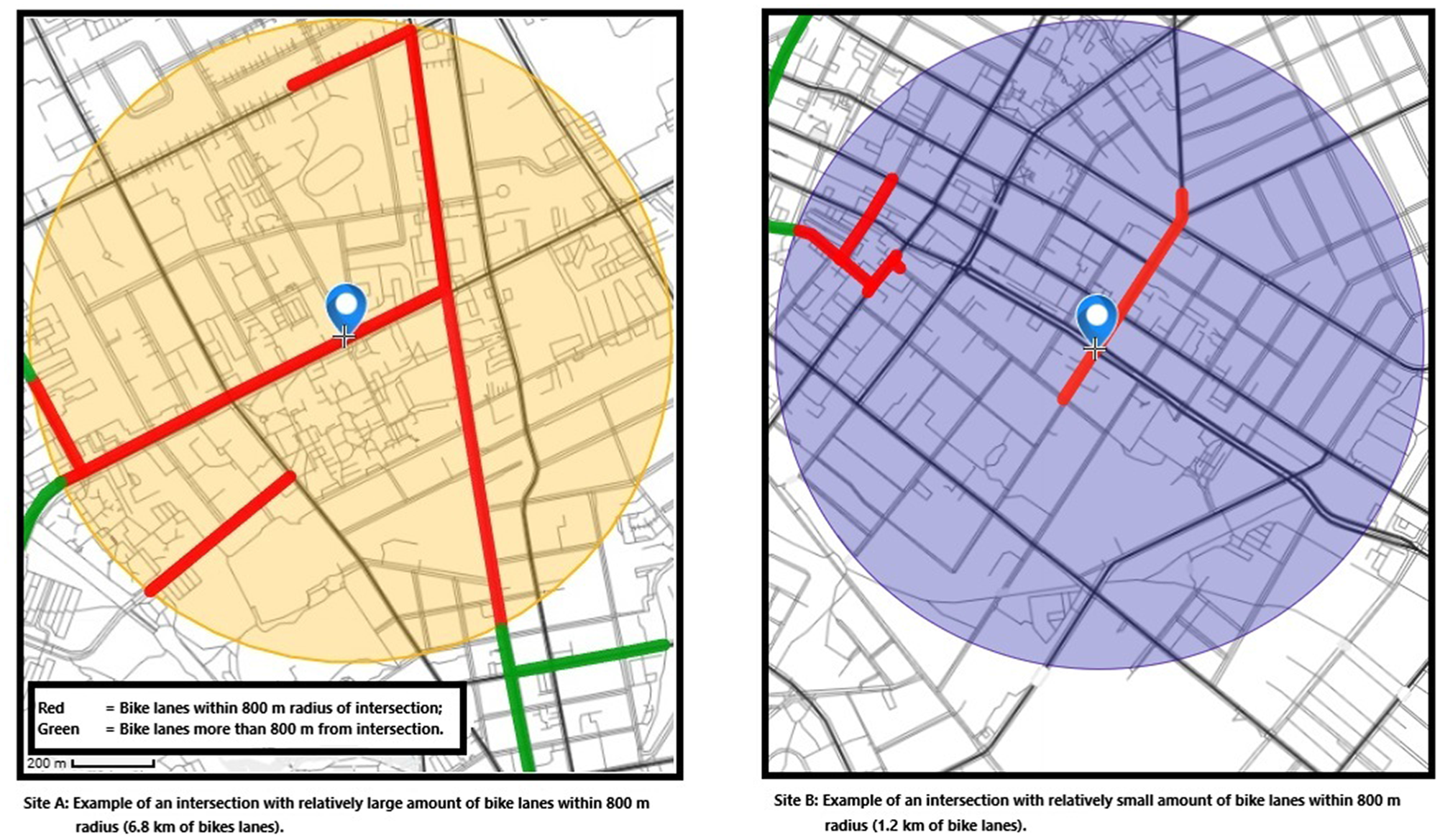
Image provided to survey participants to illustrate “total length of bike facilities”, feature variable.
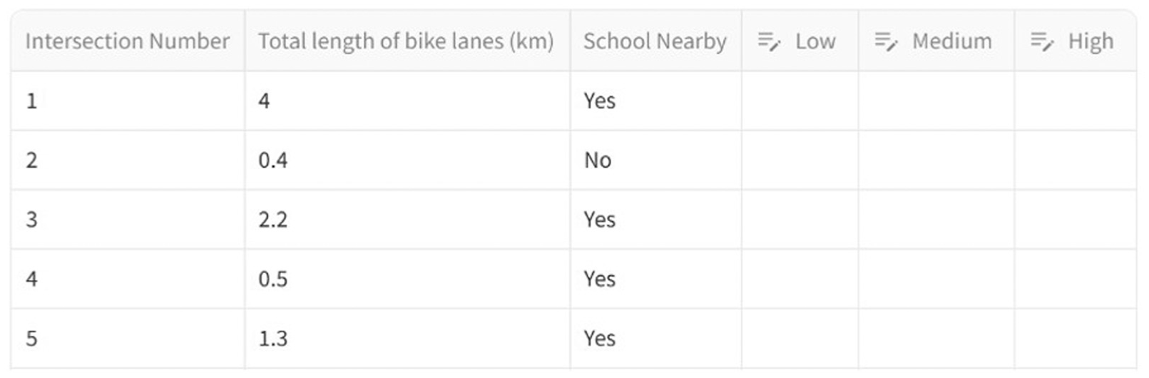
Sample of the survey questionnaire.
Results and Discussion
This section is organized into three subsections. The first subsection presents the performance of the Naïve benchmark model and the development and performance of the OL benchmark model. The second subsection presents the performance results of the LLMs. The third subsection presents the results of the survey, demonstrating the performance of humans as a further benchmark for assessing the performance of the LLMs.
Comparison Models
Naïve Model (BM1)
The Naïve model (BM1) randomly selects an AADB category for each site and is presented as the minimum accuracy threshold that must be surpassed by any proposed model (including LLMs). In this study, the AADB is categorized into three levels, and there are an equal number of sites (25) in each AADB category. The accuracy of each application of the Naïve model varies because of randomness; however, the average accuracy of the Naïve model should be 33%. The application of the Naïve model 30 times resulted in an average accuracy = 35%.
OL Benchmark Model (BM2)
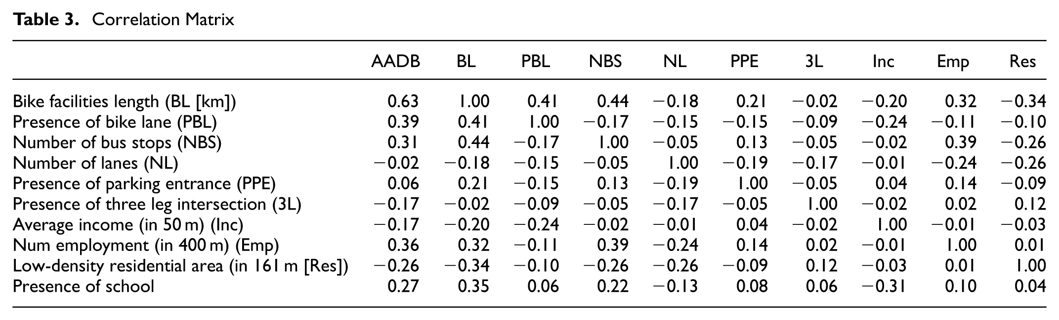
The OL model was calibrated on the study data set. Equations 7–10 represent the OL model to extract the continuous latent variable and the corresponding probability calculation for each category. The fit criteria were to select a model that minimizes the AIC criteria while maximizing the accuracy from the confusion matrix. The correlation matrix for the site features is provided in Table 3. From this table, site features can be identified that are highly correlated with each other (colinear) and those that are strongly correlated with the dependent variable AADB (e.g., bike facilities length [BL], presence of bike lane, number of bus stops, employment [Emp], and schools). The best fit OL model included just two independent variables, BL and Emp and two thresholds (τLow/Medium and τMedium/High). Model fit and coefficient values are provided in Table 4.

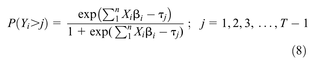
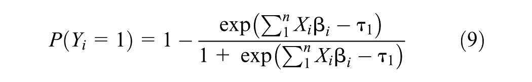
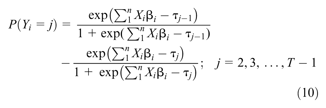
where
Correlation Matrix
Ordered Logit Model Calibration Results
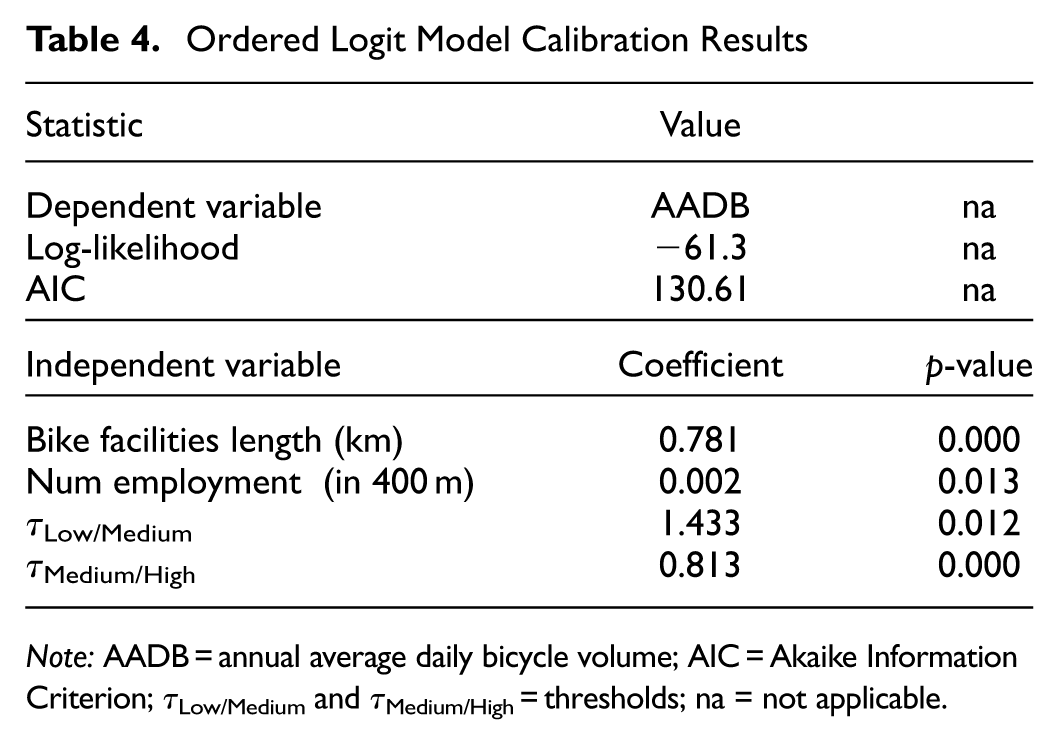
Note: AADB = annual average daily bicycle volume; AIC = Akaike Information Criterion; τLow/Medium and τMedium/High = thresholds; na = not applicable.
Categorization by Humans (H1)
As mentioned in the Methodology section, a survey was conducted in which respondents were given values for two site features (total length of bike facilities within 800 m of the site and whether or not a school was located within 400 m of the site) and asked to categorize the level of bicycle volume at the site. Respondents were asked to do this categorization for 75. The survey was distributed online, with a brief explanation of its purpose. The survey took approximately 10–15 min to complete. The target sample size was 30, to match the number of LLM replications. No personal information was collected; only estimation results for all 75 sites were gathered, similar to the LLM tests.
The average accuracy from the 30 survey respondents was 52%, which is much better than the Naïve model and ranges from approximately 0.4 to 0.6.
LLM Models
Based on the explanatory variables described in the Site Features section, the correlation analysis in the previous section, and features found to be statistically significant in the logit model, various models were tested using the OpenAI API. Details of the variables selected for each model are provided in Table 5. As explained in the Methodology section, three main hypotheses were tested for the LLM models to examine their potential use in providing the highest average accuracy over 30 replications and their compatibility with traditional benchmark models.
Model Scenario
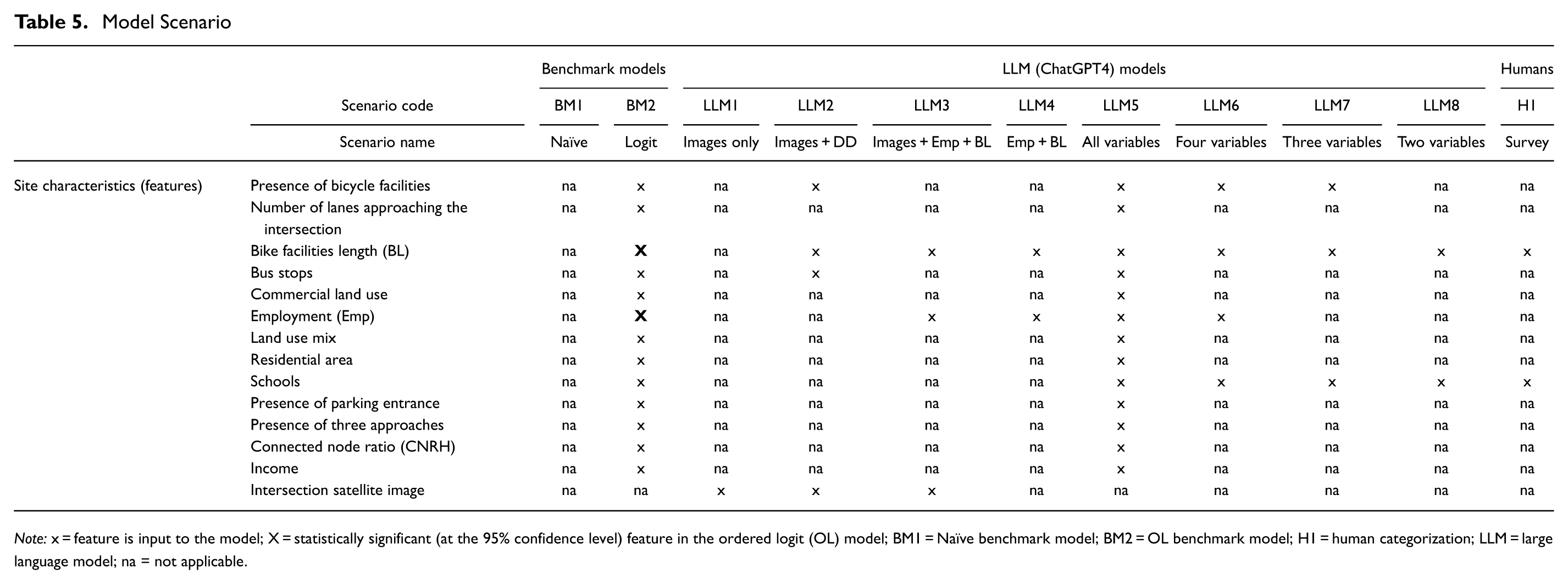
Note: x = feature is input to the model; X = statistically significant (at the 95% confidence level) feature in the ordered logit (OL) model; BM1 = Naïve benchmark model; BM2 = OL benchmark model; H1 = human categorization; LLM = large language model; na = not applicable.
The average accuracy, based on confusion matrices, was calculated for all LLM models and the comparison models, as shown in Figure 6. The highest accuracy was achieved by the benchmark (OL) model, with 64%. The second-best performance came from the ChatGPT model (accuracy = 60%), which utilized only two variables (bicycle facility length and presence of schools) and no images (LLM8).
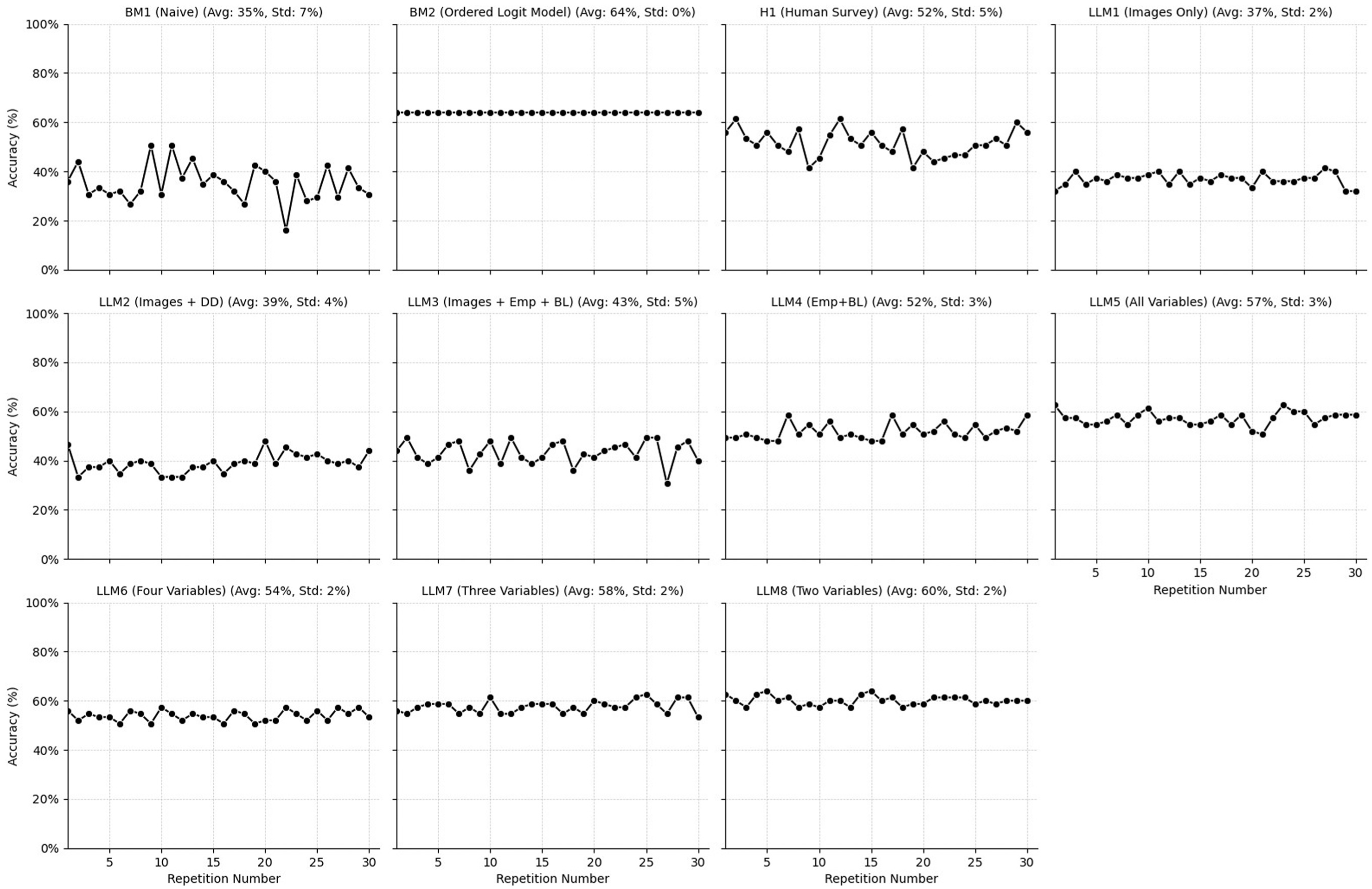
Accuracy comparison across all models.
Statistical tests were used to determine whether the differences in average accuracy between different pairs of models are statistically significant. The F-test was used to compare the variances. If the variances were statistically different, then the independent two-tailed t-test assuming unequal variances was used, the independent two-tailed t-test assuming equal variances was used.
Table 6 presents the t-value results of independent two-tailed t-tests for each pair of models. For all comparisons, the critical t-value = 2.045. The three cells with bolded text indicate model pairs that are not statistically significant; all other results are statistically significant at the 95% confidence level. The findings indicate that all LLM models without images outperform the model with images, and these differences are statistically significant. With the exception of LLM1 (Images Only), all other models have average accuracies that are statistically better (t-values are positive and greater than 2.045) than the Naïve model (BM1). This is surprising because the Naïve model represents a low bar for performance. More interesting is that the average accuracy of the human participants was (statistically) higher than some of the LLM models (specifically, the LLM1 (Images Only) and LLM2 (Images + DD), both of which include images.
Student t-values from Independent Two-Tailed t-tests for Each Pair of Models
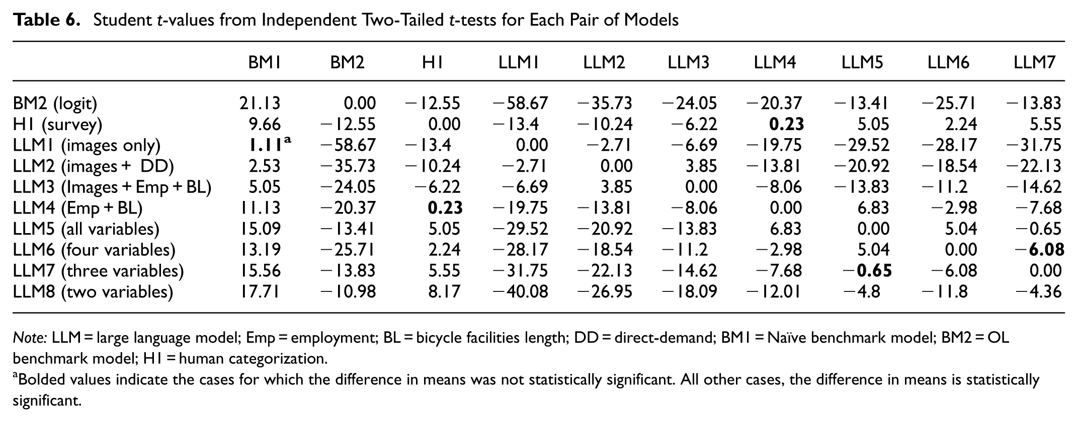
Note: LLM = large language model; Emp = employment; BL = bicycle facilities length; DD = direct-demand; BM1 = Naïve benchmark model; BM2 = OL benchmark model; H1 = human categorization.
Bolded values indicate the cases for which the difference in means was not statistically significant. All other cases, the difference in means is statistically significant.
The best-performing LLM relies solely on two inputs: BL and the presence of schools. An examination of the correlation matrix in Table 3 highlights that these two features have a strong correlation with the AADB, and bicycle facility length was a statistically significant variable in the ordered probit model. The presence of schools is frequently a statistically significant variable in DD models for estimating pedestrian and bicycle volumes; therefore, its presence is not surprising. In addition, this study’s jurisdiction contains three post-secondary educational institutions (two universities and one college), which are likely to be generators and attractors of bicycle trips.
Five research questions were posed in the Methodology section. The model application results are used to answer these five questions.
Question 1: Does the LLM Perform Better than Randomly Assigning Volume Categories (Naïve Model)?
The results show that all tested LLMs, except the LLM with only satellite images as input (LLM1), outperform the Naïve model in accuracy, and the difference is statistically significant.
Question 2: Is the LLM Performance Comparable with Traditional Methods, such as Statistical Approaches and Human Survey Analysis?
A comparison analysis between traditional statistical methods, such as developing an OL model (BM2), indicates that LLMs in general can achieve very similar levels of accuracy. For instance, LLM8, using only two variables, achieves an accuracy of 60%, and BM2, using very similar variables, reaches an accuracy of 64%. A comparison between the LLM and human survey analysis (H1) shows that LLMs can outperform humans in accuracy. For example, LLM8 achieved an average classification accuracy of 60%, and the average accuracy from the human survey was only 52%. This is a positive outcome because the survey design closely mirrored the structure of the input prompts provided to the LLMs.
Question 3: Does Providing Satellite Images Improve LLM AADB Categorization Accuracy?
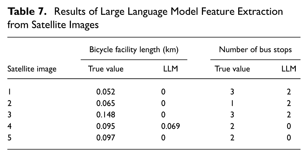
The results shown in Figure 5 and listed in Table 4 indicate that LLMs without images (LLMs 4–8) outperformed those with images (LLMs 1–3). The differences in accuracy for the LLM models without images were statistically significant, and their average accuracy was higher than that of the models with images. Therefore, the results indicate that providing LLMs with satellite images of the sites does not improve the average accuracy of category classifications. This result is somewhat surprising because it might be expected that the spatial distribution of site characteristics would be helpful in estimating the AADB category. It was hypothesized that the LLM could not accurately extract features from the image, and the errors in the feature extraction had a detrimental effect on AADB estimation accuracy. This hypothesis was tested by providing an image (the same image size as used in the rest of this study) to the LLM and prompting the LLM to assess the image and provide two features: (1) the number of bus stops present in the image; and (2) the length of bicycle facilities (e.g., bike lanes and multiuse paths) in the image (in km). This analysis was repeated for five randomly chosen sites in the data set. The results (Table 7) confirmed the hypothesis that the LLM is unable to accurately extract important land use features from the provided satellite images. Bicycle facilities exist at all five tested sites; however, the LLM detected bike facilities at only one of the sites, and even at this site, it incorrectly determined the length of the facility. There were bus stops at all five sites, but the LLM detected bus stops at only three of the five sites, and at all three sites, the extracted number of bus stops was incorrect.
Results of Large Language Model Feature Extraction from Satellite Images
Question 4: Does Providing More Site Feature Variables Within the LLM Prompt Improve LLM AADB Categorization Accuracy?
The results indicate that LLMs, with a higher number of explanatory variables, were less accurate than those with fewer variables. This is somewhat surprising, and it might be related to how LLMs interpret input data because they seem to rely more on context-based information than on the numerical input values as explanatory variables. In addition, adding more variables might make interpretation more complex for LLMs.
Question 5: How Stable is the LLM Performance Across Different Sites (i.e., Are Results Affected by Overfitting to the Specific 75 Sites Used in this Study)?
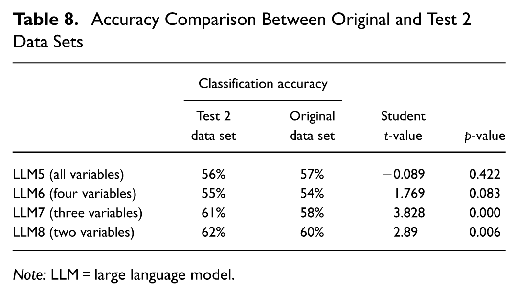
This question is difficult to answer definitively without compiling an entirely separate data set, which was unavailable. Instead, overfitting was evaluated using another set of 75 sites from the same jurisdiction (Test 2 data set, as described in the Methodology section). Only a subset of the LLMs (LLM5–8) were applied to the Test 2 data set because these models performed much better than the other LLMs. The findings show that overfitting was not an issue, as very similar results—and in some cases, higher average accuracy—were achieved by the LLM models on the Test 2 data set. An independent two-tailed t-test was conducted to compare the mean accuracy of Test 2 with the original data set. The results indicated that there is no statistically significant difference between the mean accuracy of LLM5 and LLM6. However, the mean accuracies of LLM7 and LLM8 were significantly different, with a higher mean accuracy for the Test 2 data set. This finding may be attributed to the sample size of 30 and because both data sets share the same sites for the High bicycle volume category. A comparison analysis of prediction accuracy between Test 2 and the original data sets is given in Table 8.
Accuracy Comparison Between Original and Test 2 Data Sets
Note: LLM = large language model.
Conclusions and Recommendations
This study aimed to answer five specific research questions as discussed in the previous section. The main conclusions from this work are as follows.
ChatGPT exhibited statistically significant higher average bicycle volume classification accuracy than the Naïve model (average accuracy = 35%) for almost all input data combinations examined (the only exception being the LLM using only satellite images as input).
The best-performing LLM (LLM8) required only two site characteristics as inputs (total length of bike facilities within 800 m of the intersection and number of employment within 400 m of the intersection) and provided an average classification accuracy of 60%. The best-performing LLM (LLM8) provided average classification accuracy (60%) that was significantly better than the Naïve model (35%) and human survey respondents (52%). Furthermore, this LLM performed almost as well as the statistical model (OL model) developed on this same data set (accuracy = 64%). The findings of this study show that the LLM model can perform almost as well as traditional DD models. This is promising because, compared with traditional DD models, the LLM model requires less time and cost for development, as well as for data collection and analysis.
An examination of the effect that inputs have on the LLM performance indicated that the use of quantitative inputs, rather than satellite images, improved classification accuracy. This suggests that ChatGPT is unable to accurately extract relevant land use, demographic, or transportation network characteristics directly from satellite images. Furthermore, providing a higher number of quantitative features (variables) as input to the LLM tended to lower the average accuracy, with reductions from 2.5% to 6.3% and an average decrease of approximately 4% compared with the best-performing model, which uses only two variables. All models with more variables were statistically less accurate than the two-variable model. Efforts were made to determine whether results were affected by overfitting. The analysis showed that overfitting is not an issue; however, limitations in the number of sites for which AADB data were available precluded the compilation of a completely different data set on which to test for overfitting.
Overall, LLMs present substantial promise as a tool for estimating bicycle volume levels. The models do not require extensive input data, and they are readily available at low cost.
This study and its findings have several limitations.
The variables used in this study are not guaranteed to provide the highest average accuracy when used in other jurisdictions.
The number of AADB categories and the associated AADB boundary values to define the categories were developed relative to the jurisdiction used for this study. Therefore, they are not necessarily applicable to other jurisdictions with different characteristics.
It is recommended that the use of LLMs for estimating bicycle volume levels be further evaluated as follows.
Applying LLMs to data sets from other jurisdictions to examine the spatial transferability of LLMs and the optimal set of inputs.
Exploring the ability of LLMs to classify bicycle volume levels at locations other than intersections, which is the focus of this study (e.g., mid-block locations or links).
Examining the potential to improve LLM classification accuracy by training a special-purpose LLM.
Evaluating the performance of LLM classification compared with traditional ML approaches, such as XGBoost or RF.
Footnotes
Acknowledgements
The authors gratefully acknowledge the Region of Waterloo, Ontario, Canada, for providing permission to use the bicycle count data and for providing rich open data portals that were essential sources of information for this research and Miovision for providing access to the bicycle data. The work in this study reflects the views of the authors, and there is no explicit or implicit endorsement by any of the aforementioned jurisdictions or companies.
Author Contributions
The authors confirm contribution to the paper as follows: study conception and design: Hellinga, Azizi Soldouz; data collection: Azizi Soldouz; analysis and interpretation of results: Azizi Soldouz, Hellinga; manuscript preparation: Azizi Soldouz, Hellinga. All authors reviewed the results and approved the final version of the manuscript.
Declaration of Conflicting Interests
The authors declared no potential conflicts of interest with respect to the research, authorship, and/or publication of this article.
Funding
The authors disclosed receipt of the following financial support for the research, authorship, and/or publication of this article: The authors gratefully acknowledge financial support from the Natural Sciences and Engineering Research Council of Canada via the Discovery Grant Program (funding reference number 2022-03275) and Transport Canada’s Enhanced Road Safety Transfer Payment Program. The research was carried out by the authors, and no endorsement of the methods or findings by funding agencies is claimed or implied.