
Abstract
Ride pooling services are considered as a customer-centric mode of transportation, but, at the same time, an environmentally friendly one, because of the expected positive impacts on traffic congestion. This paper presents an analytical model that can estimate the traffic impacts of ride pooling on a city by using a previously developed shareability model, which captures the percentage of shared trips in an area, and the existence of a macroscopic fundamental diagram for the network of consideration. Moreover, the analytical model presented also investigates the impact that improving the average velocity of a city has on further increasing the percentage of shared trips in an operation area. The model is validated by means of microscopic traffic simulations for a ride pooling service operating in the city of Munich, Germany, where private vehicle trips are substituted with pooled vehicle trips for different penetration rates of the service. The results show that the average velocity in the city can be increased by up to 20% for the scenario when all private vehicle trips are substituted with pooled vehicle trips; however, the improvement is lower for smaller penetration rates of ride pooling. The operators and cities can use this study to quickly estimate the traffic impacts of introducing a ride pooling service in a certain area and for a certain set of service quality parameters.
Keywords
Our cities are experiencing growth in population every year, which contributes to increased traffic demand. The use of private vehicles—even though convenient—is not sustainable, considering the large amount of parking space and street capacity that is required as a result of an average occupancy of only 1.3 passengers per vehicle ( 1 ). From the other side, traditional public transportation is typically an efficient and environmentally friendly mode of transportation; however, it may not be very attractive for customers because of the lack of convenience and flexibility as a result of fixed line and schedule and a limited area of coverage.
The extended availability of smartphones and data accessibility have made possible the emergence of ride pooling services. These services offer a user-centric and sustainable mobility option for the customer, which can reduce the vehicle kilometers traveled in the system because of sharing of trips with similar trajectories ( 2 – 4 ). However, an effective ride pooling service depends largely on the customers’ readiness to use it, which is affected by individual choices and on the attributes of the service. The service attributes which affect customers the most are travel time, waiting time and service cost, and the lower they are, the higher is the attractiveness of the service ( 5 ).
From the operators’ perspective, the percentage of shared trips in an area, called shareability, influences the profitability of the service, and therefore plays an important role in deciding whether to offer a pooling service in an area or not. Santi et al. examined shareability in a city via simulations by using the concept of shareability networks ( 6 ). To generalize the calculation of shareability for different cities, Tachet et al. established a mathematical model, in which shareability depends on city parameters (average speed and surface of the operating area) and service attributes (detour time) and tested it for different cities ( 7 ). Their model was extended by Bilali et al. to capture the additional influence of maximum waiting time, boarding time, and reservation time, and the impact that the modeling details have on shareability, showing that, in particular, the choice of the optimization objective has a high effect on shareability ( 8 – 10 ).
The before-mentioned studies derived shareability without considering the traffic impact of ride pooling. Therefore, average velocity—a commonly used measure of traffic efficiency—is assumed to be constant in space and time in these models. However, by introducing a ride pooling service in a city, the number of vehicles on the roads will decrease, thereby increasing the average velocity in the network. As the velocity is in turn an input for the shareability model, the percentage of shared trips in an area will increase even further. This effect is noted as second-order effect of velocity on shareability and its basic idea is illustrated in Bilali et al. for a synthetic grid network ( 11 ). In this paper, the concept of this second-order effect will be explored for a real city network and a more realistic analytical model capturing traffic effects of ride pooling.
The benefits of ride pooling, focusing on a particular city, have been investigated a lot by researchers. Alonso Mora et al. showed that 98% of taxi trips in New York city currently catered for by 13,000 taxis, can be substituted by a fleet of only 3,000 pooled vehicles, reducing the mean travel distance in the system ( 2 ). A study for the city of Prague, Czech Republic, substituting private vehicle trips with pooled trips, demonstrated that, when using ride pooling, vehicle kilometers will decrease to 60% of the current state ( 3 ). A similar study was performed for the city of Munich, Germany, and the authors argue that the benefits of pooling are seen only after a certain penetration rate of the service, for which the saved travel kilometers resulting from shared trips are higher than the empty vehicle trips generated to pick-up customers ( 4 ).
All of the above studies investigate only the impact from the pooled vehicle fleet and indirectly check the traffic impacts by calculating the vehicle kilometers in the system, without examining the interaction with the other vehicles that are present in the network. These studies are performed using agent-based simulations, which, even though providing a good estimation of the vehicle kilometers in the system, are specific for a particular city and require a large amount of input data. Therefore, a generalization for different city types is difficult. Albeit the traffic impacts of ride pooling are not directly investigated in these studies (as, for instance, would be the case if the agent-based simulation were to be coupled with a microscopic traffic simulation), the computational time needed for these simulations is still very high and rises with increasing problem size. Therefore, it is difficult to simulate high-demand pooling states, and it is even more difficult and time demanding to investigate the direct traffic impact by integrating the agent-based simulation and microscopic traffic simulation for the pooling case.
To overcome the drawbacks of using agent-based simulations and to be able to estimate quickly the impact of ride pooling with only a little input data, this paper presents a method to derive analytically the traffic impacts of ride pooling services. The main requirement is the existence of a macroscopic fundamental diagram (MFD) for a specific city. Additionally, the influence that the improvement of average velocity in the city has on shareability is also modeled. The models presented in this paper are tested for the city of Munich using AIMSUN as a microscopic simulation environment.
Analytical Model
This section describes a model allowing the analysis of traffic impacts of ride pooling. Firstly, an introduction to the shareability model is given, followed by a model for the reduction of vehicle trips in the road network resulting from shared trips. Subsequently, the relation between average velocity and vehicle trip generation and the modified shareability model are described. A detailed description of the model parameters can be found in Table 1.
Model Parameters
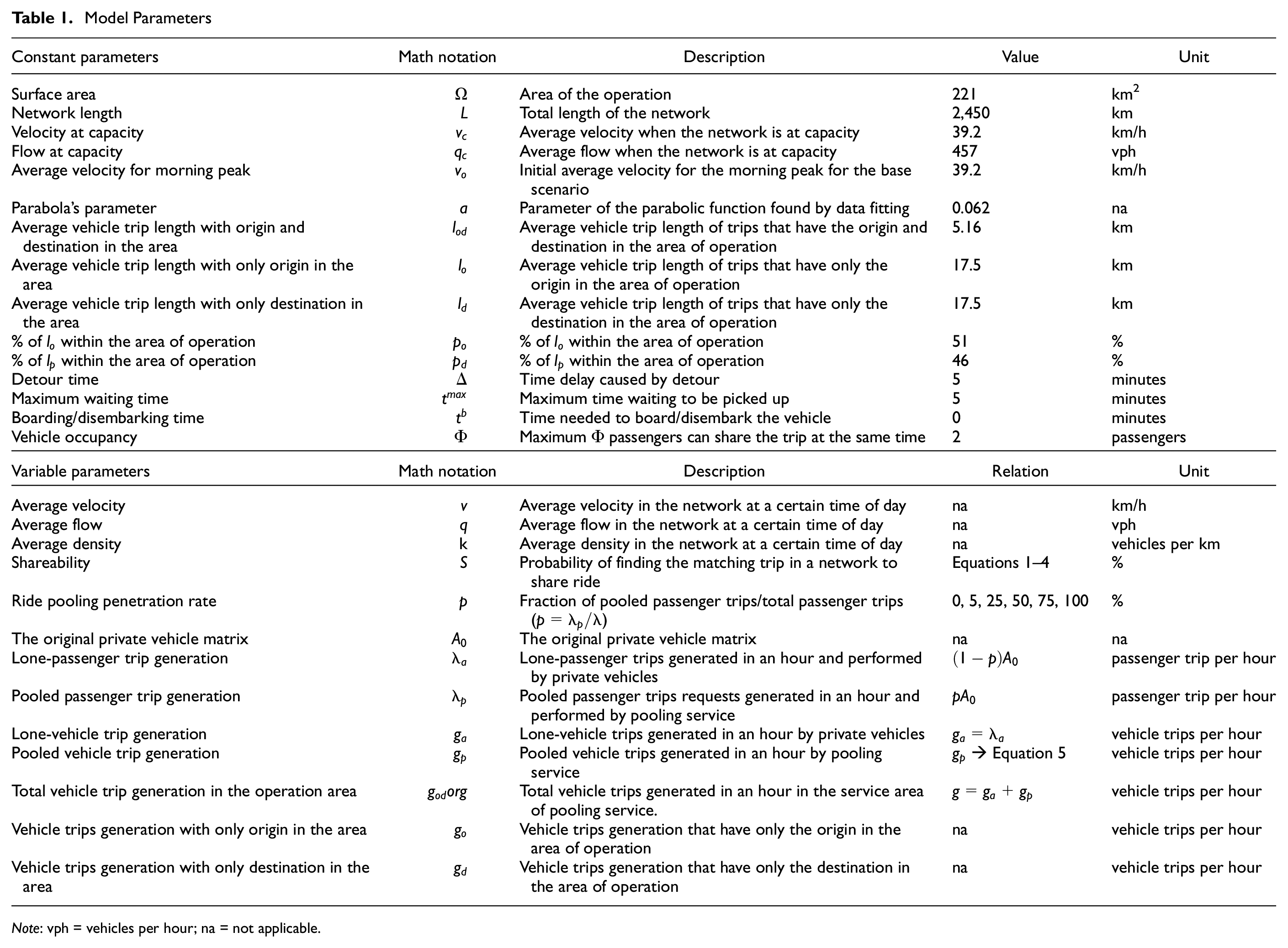
Note: vph = vehicles per hour; na = not applicable.
Shareability Model
The benefits of ride pooling are reliant on the possibility of sharing trips which have similar trajectories. The percentage of shared trips in an area is called shareability
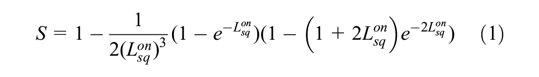
where the dimensionless quantity
The calculation of shareability is based on the notion of the shareability shadow, which defines the geometric shape of where in space the origins and destinations of a trip should be to be shareable with an already existing trip, without violating the time constraints (defined by service quality parameters) (
7
). Depending on the relation that service quality parameters have with each other, there are two different shapes of the shareability shadow specified by Bilali et al. and, therefore, two forms of
For
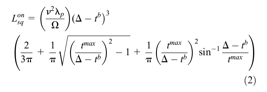
and for
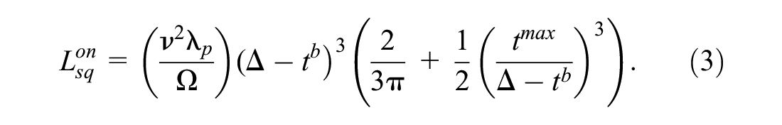
The above equations determine the value of shareability when the optimization objective in the customer matching problem is to maximize the percentage of trips which will be shared ( 8 ). However, using the objective of maximizing the percentage of shared trips does not necessarily mean that the distance traveled is minimized. To maximize the percentage of shared trips, the pooling algorithm might decide about sharing of the trips (when the time constraints allow it) just for the sake of achieving maximum percentage of shared trips, even though it might be more effective in relation to saved vehicle kilometers to serve the customers one after the other ( 10 ).
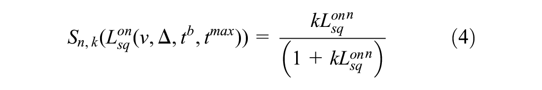
As the optimization objective to minimize vehicle kilometers traveled is more favorable to improve the traffic conditions, it is the one selected in this study. The shareability for this optimization objective is given by a prediction model defined by Bilali et al. and inspired by Santi et al. and shown in Equation 4 (
6
,
10
). This form of equation also describes statistically the natural combinatorial effects of particle bonding processes in biochemistry. To use this prediction model, the results of the shareability values derived by means of simulations for a base scenario referring to a certain set of service quality parameters are needed. Therefore, by fitting the simulated shareability data to the form of shareability equation given by Equation 4, the parameters n and k are defined. To calculate the shareability for another set of service quality parameters, the parameters n and k are kept the same and the impact of the new service quality parameters is reflected in the
This shareability model returns the percentage of shared passenger trips in an area, while assuming that the average velocity in the city
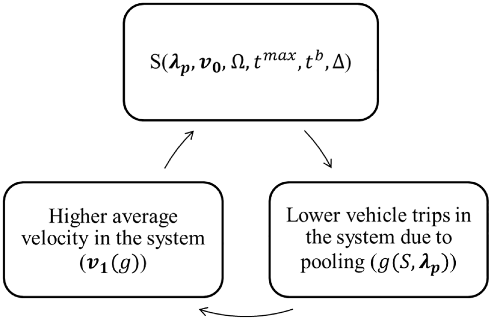
Additional effect of average velocity on shareability.
Vehicle Trip Reduction Model
A distinction is made between passenger trips generation rate

Therefore, the total number of vehicle trips per hour in the system
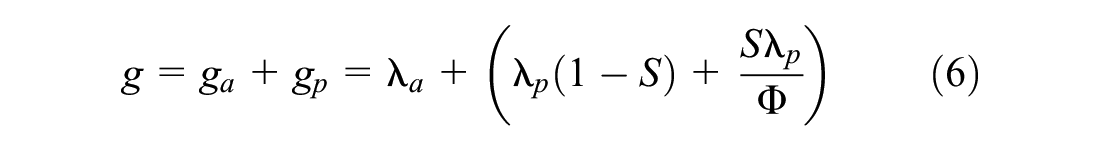
This reduction in total vehicle trips in the system is expected to improve traffic conditions in the city by improving the average velocity.
Analytical Relation of Average Velocity and Vehicle Trip Generation
As previously mentioned, reducing the number of vehicles in the system will affect the average velocity in the city. This section will present an analytical model to capture the relation of average velocity and vehicle trip generation by exploiting the benefits of an MFD. Therefore, it will be possible to analytically derive the improvement in average velocity coming as a result of the reduction of vehicle trips in urban areas because of ride pooling.
Macroscopic Fundamental Diagram (MFD)
MFD (or network fundamental diagram) defines the functional form of the relation between average velocity, traffic flow
The functional form of MFD is also going to be exploited in this study and used as a basis for defining the relationship between average velocity and vehicle trip generation in a network. The MFD for this study is derived by means of simulations. For each time interval, I, the average velocity


As the relation of flow and velocity resembles a parabola, to connect these two parameters analytically, a parabolic function is defined in the form given by Equation 9, where the vertex of the parabola is V(

Analytical Vehicle Trips in a Network Based on MFD
Firstly, a simple method to define the traffic density of a network analytically will be described. It is assumed that a ride pooling service will be operated in an area defined by a boundary, as illustrated in Figure 2. Within this area, there are three different types of trip to be considered: (1) the ones that have the origin and destination within the area, (2) the ones that have the origin in the area and the destination outside, (3) the ones that have the destination in the area and the origin outside, and (4) the trips that have both origin and destination outside the operation area but pass through it. The first type of trip includes the lone-vehicle trips and the potential pooled vehicle trips. The second and third types of trip are the ones that comprise what will be called here “background traffic” in the network as they are going to be there regardless of the impact of the ride pooling service in vehicle trip reduction, as the impact that might come from parking in the boundary of the area of service and continuing the trip with ride pooling service is neglected in this study. To define the traffic density within the boundaries of this area, only the contribution of vehicle trip types (1), (2), and (3) are considered, and the contribution from type (4) is left out, as most of the cities have a highway belt to reduce transit traffic within the city.
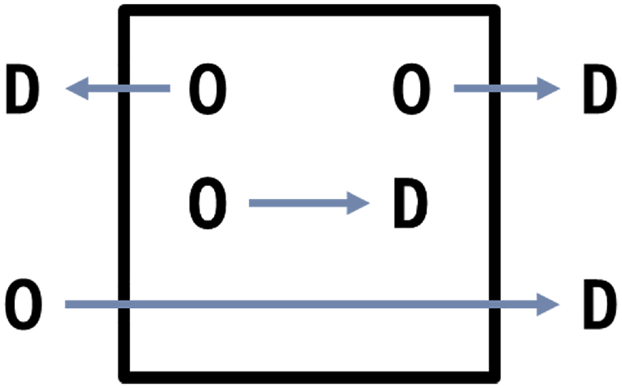
Illustration of an operating area with position of origin–destination (OD) trips.
Traffic density is defined as the number of vehicles per lane kilometer in the system. According to Little’s law the average number of vehicles in the system is equal to the average time the vehicles spend in the system multiplied by the average number of vehicles generated (
23
). If only the vehicles of type (1), which have both the origin and the destination within the area of operation, are considered, the traffic density

where
For vehicle trips of type (2) and (3), which have only their origin or destination within the area, the background density

where
As the vehicle trips of this type are only partly inside in the area,
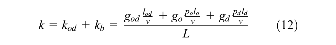
The overall network’s traffic density is the sum of the traffic density of vehicle trips type (1), (2), and (3), as illustrated in Equation 12.
From the MFD relation,

From Equation 13 it is possible to derive the generated number of vehicle trips of type (1), which have both the origin and destination in the operated area

By substituting
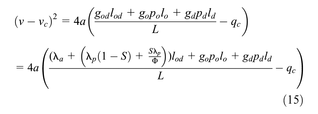
If
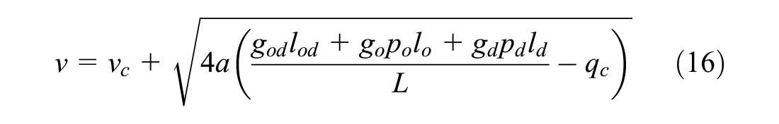
And if
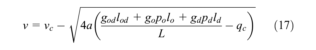
In this way, it is possible to derive the new average velocity in the network, only by having knowledge of the MFD and the reduced number of vehicle trips per hour resulting from pooling, calculated by Equation 6 when shareability value is known. The parabolic shape of this relation is also supported by a recent study from Ke et al. ( 24 ).
Modified Shareability Model
By capturing the impact that ride pooling has on improving average velocity in the network, this study also captures the additional impact that the change in average velocity has on the shareability value. Therefore, this part describes the modified shareability model where, different from previous studies, velocity is considered as a dynamic parameter.
To define the modified shareability value, the dynamic velocity formulation, which depends on shareability, given in Equation 15, is substituted into the shareability Equations 2 and 3. Therefore, the modified
For
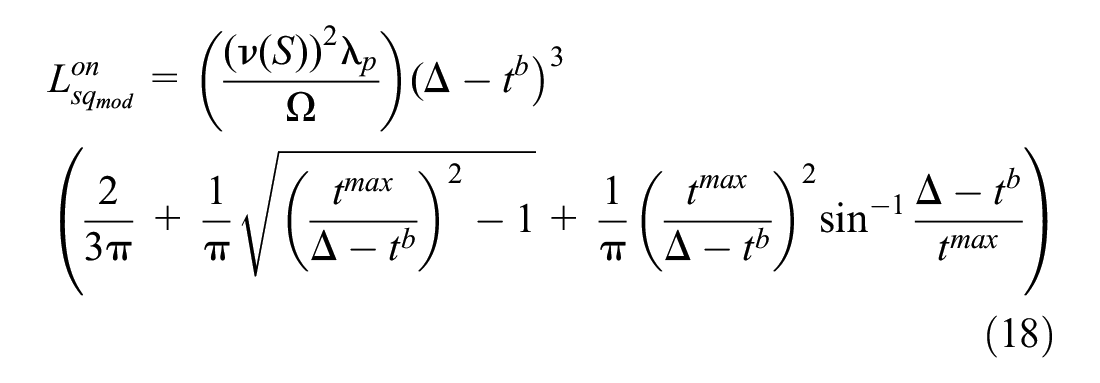
and for
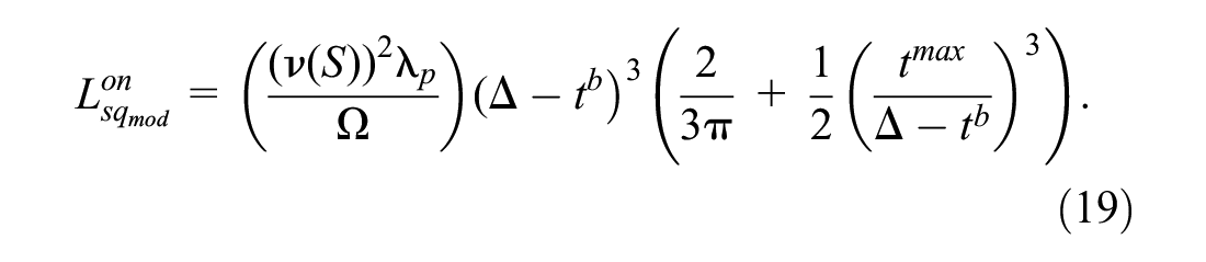
Substituting
The model described in this section can capture analytically the traffic impact that ride pooling has on average velocity and the improvement that it may additionally cause to the urban environment because of the additional increase of shareable trips. This implies that traffic improvement resulting from ride pooling will also be beneficial for operators to increase the chances of finding shareable trips as a result of further distances reached within the allowed detour time because of higher velocity.
Simulation Setup
Operating Area
To validate the developed model and investigate the traffic impact of introducing a ride pooling service, a ride pooling service in the city of Munich is considered, where private vehicle trips are substituted with pooled vehicle trips for different penetration rates of the service. The Munich network is built in the microscopic traffic simulation environment AIMSUN (
26
). The operating area considered (Figure 3) is located around Munich city center, similar to the one in Bilali et al. (
10
). Its surface is 221 km2 and the network length
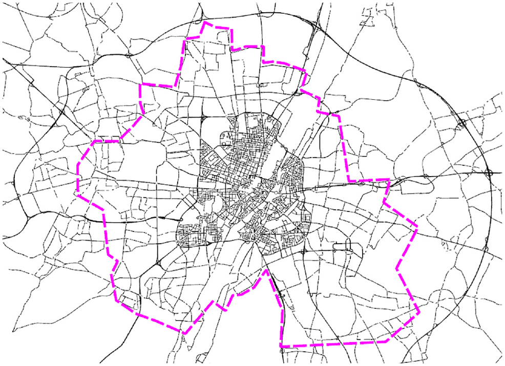
Munich operating area.
To construct the MFD for this network and extract the relevant information, microscopic simulations are run for the time period from 06:00 to 24:00. To push the network to capacity, two other simulations are also run for scenarios where the private vehicle trip demand is increased by 10% and 20%, respectively. One (network average) flow-velocity data point is extracted every 10 min based on Equations 7 and 8, and it is plotted in the MFD graph.
Scenario Setup
To test the impact of pooling for a more congested network, the traffic demand of the base scenario is selected to be 10% higher than the current demand from private vehicle trips in Munich and it is assumed that the pooling service is offered during the morning peak time from 07:00 to 10:00. The simulation for the base scenario is run, the results are extracted every 10 min, and the average velocity in the network for each time interval is obtained by using Equation 7. The average velocity for the morning peak time
To investigate the traffic impacts of a ride pooling service offered within the area of Figure 3, private vehicle trips type (1) are substituted by pooled vehicle trips for different scenarios, where the penetration rate of ride pooling service
To model these pooling scenarios in AIMSUN, a distinction is made between the traffic demand generated in the network from different vehicle types, and three origin–destination (OD) matrices are created: matrix (B) for the background traffic (vehicle trips type [2], [3] and [4]), matrix (A) for the private (lone) vehicle trips type (1) (
It is assumed that private vehicle and ride pooling trips follow the same OD distributions and scale as the demand matrices based on


For the ride pooling service selected in this study, where the optimization objective used by the operator for the matching algorithm is to minimize the vehicle kilometers traveled in the system, shareability in the area is derived by using Equations 2–4. The area of the city
For each scenario, one simulation is run for the morning peak time 07:00 to 10:00 and the network statistics are extracted every 10 min. Similar to the base scenario, the average velocity in the network is calculated for each time interval by using Equation 7 and then it is averaged for the morning peak time. All the model parameters and values are shown in Table 1.
Results
Macroscopic Fundamental Diagram (MFD) for Munich Network
The MFD for the operating area in the city of Munich is shown in Figure 4. As specified in the Scenario Setup section, the blue data points to construct this MFD were extracted from the results of three scenarios with different demand levels. The virtual queues of the vehicles waiting to get into the network are kept at minimum to control the state of the network and make sure that network gridlock, which might occur when the input flow exceeds the supply function, is not happening.
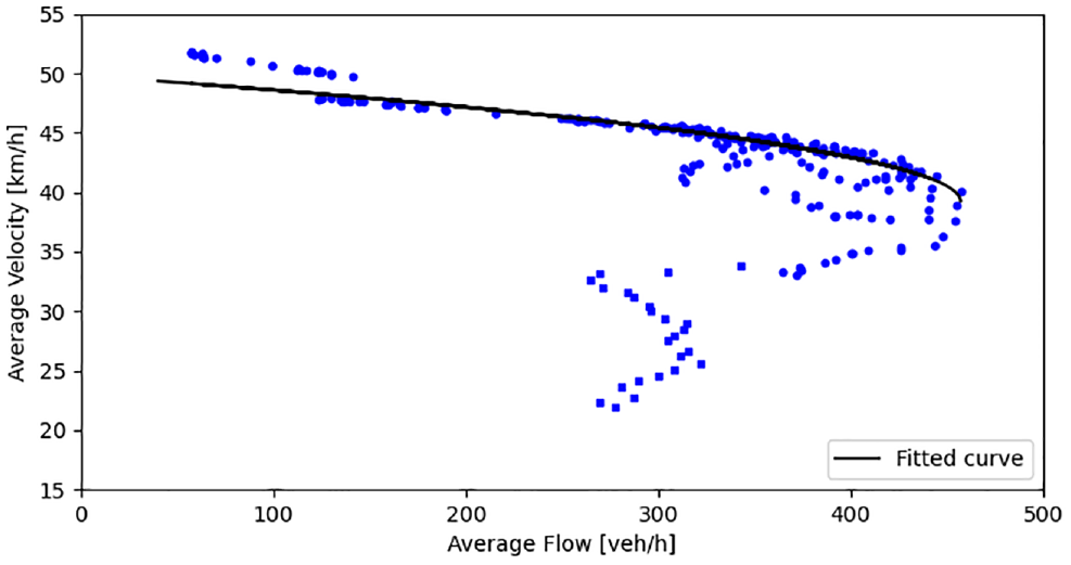
Macroscopic fundamental diagram (MFD) for Munich.
The x-axis correspond to the value of average traffic flow and the y-axis corresponds to average velocity. It is shown that the area of consideration from the Munich network is at the free flow state most of the time, while reaching the unstable state at the network’s capacity during the peak times. This form of the MFD for the city of Munich is similar to the one observed in Dandl et al. (
28
). The high average velocity values come as a result of the large area considered, which contains city highways and arterials, where the speed limit is high. A clockwise hysteresis loop is observed for the investigated scenarios caused when the demand starts decreasing after the peak time, showing that the system does not return to the free flow state immediately if the initial congestion level in the network is high (
16
). Therefore, the hysteresis phenomenon in this study occurs when, for the same average flow in the network, the average velocity is higher during the congestion onset compared with its values during the congestion offset. Geroliminis and Sun show that one reason for the occurrence of this phenomenon is the dissimilar spatial and temporal distribution of traffic congestion (
29
). The correlations of the loop size of the MFD, congestion heterogeneity, and network performance are further examined in Hemdan et al. (
30
). At the point where the traffic flow is at maximum at the MFD graph, the network is in its optimum state and the network’s traffic flow at capacity
To get a functional form for this MFD, the equation of parabola specified in Equation 15 is used. As the majority of the data points belong to the free flow state and the base scenario has data points only in this state, the data is fit to the parabolic function defined in Equation 16 for
Average Velocity and Vehicle Trip Generation Relation
Network Information
To express the relation of average velocity and vehicle trip generation, it is necessary to extract the network information mentioned in Equation 14, namely trip lengths and percentage of the trip length inside the operating area for different vehicle trip types, for the base scenario.
To get the length of the vehicle trips type (1), (2), and (3), the centroid statistics in AIMSUN are used. The centroids within the area of operation are extracted, and the total number of vehicle trips type (1), (2), and (3), and the total kilometers traveled by each of these vehicle trip types, are calculated. By dividing the total kilometers performed by each vehicle trip type with the total number of vehicles of the respective type, the average trip length for the vehicle trips type (1), (2), and (3) is calculated to be 5.16 km, 17.5 km, and 17.5 km, correspondingly.
As vehicle trips type (2) and (3) are only partly within the area of operation, it is necessary to find the percentage of their trip length that contributes to the road network traffic within the area. Therefore, all possible paths connecting each origin with each destination are excerpted, and only the ones which start or end within the operation area are filtered. For the path that is mostly used by the vehicles, the identification numbers and lengths of the sections are obtained, and whether these sections are within or outside the area of operation is checked. The length of the trip performed within the area will be similar to the sum of the length of the sections which are situated inside the area. Dividing the vehicle trip length within the area by the total vehicle trip length returns the percentage of the vehicle trip length that is inside the operation area. In this case, the values are 51% and 46% for vehicle trips type (2) and (3), respectively.
Average Velocity and Vehicle Trip Generation Relation
The relation between average velocity and vehicle trip generation per hour for the vehicle trips which have both their origin and destination within the area (
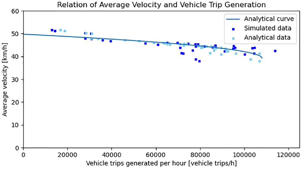
Relation of average velocity
For the simulated data points, it can be seen that there are a few scattered data points, which belong to the unstable state of the network and correspond to the hysteresis shown in MFD in Figure 4. Comparing the simulated data points with the analytically derived ones, it is possible to see quite a good correlation between them, denoting that the analytical formulation for defining the generated vehicle trips in the network based on network and trip information holds for the free flow state of the network. Further investigations are, however, needed for the congested state of the network to check the validity of the model also for this state. As this is not the case for the network in this study, it is not considered.
The analytical function relating average velocity and vehicle trip generation (
Traffic Impacts of Ride Pooling
To investigate the traffic impacts of ride pooling service, various scenarios are designed, where the penetration rate of ride pooling service
Figure 6 depicts the average velocity every 10 min for the morning peak hour for different penetration rates of ride pooling. It is observed that, at the beginning of the morning peak, when the network is not in congested state even for the base scenario, there is no significant improvement of average velocity in the network for all the scenarios tested. When the network starts to get congested and the average velocity starts decreasing, the benefits of pooling become noticeable. This emphasizes the advantage of pooling in improving traffic condition, especially during peak times, and shows that it is possible to see higher benefits of pooling in cities with high levels of congestion.
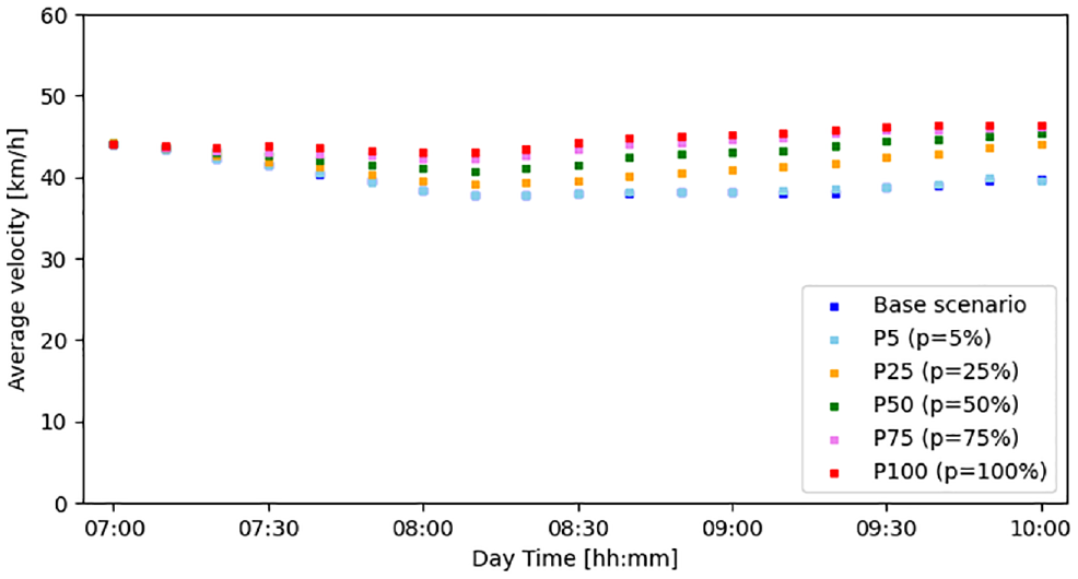
Average velocity for different pooling penetration rates.
As expected, it is shown that, the higher the penetration rate of pooling, the higher the increase in average velocity. This comes as a result of high demand for pooling, which increases the chances of finding shareable trips (shareability). Therefore, as more trips are shared, fewer vehicles are present in the road network and higher velocities are observed. Figure 7 illustrates the improvement of average velocity compared with the base scenario and shows that when the penetration rate of pooling is 100% the velocity can increase by up to 20% compared with the base scenario. For scenario P5, when the penetration is 5%, the effect of ride pooling on average velocity is quite small, indicating that when this service is introduced the effect on traffic is not expected to be seen immediately. However, with increasing market share, the positive impact of pooling will be more prominent. For instance, for scenario P25, when the penetration rate of ride pooling is 25%, the average velocity rises by up to 10% compared with the base scenario. This suggests that ride pooling services have to gain a considerable market share to profit from their positive impacts on traffic congestion.
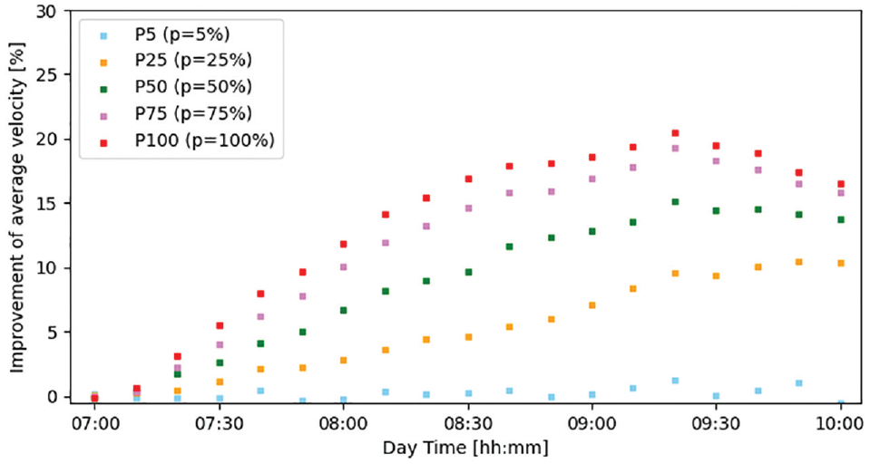
Difference in average velocity compared with the base scenario.
Modified Shareability Model
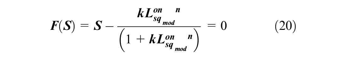
The results of the previous section show that, when private vehicle trips are substituted with ride pooling, traffic congestion is expected to improve and, therefore, the velocity will increase depending on pooled passenger demand, which effects the shareability value. Until now, velocity was considered as a constant parameter for the shareability model. Using Equations 18–20 it is possible to integrate a dynamic velocity into the shareability model and the result is illustrated in Figure 8.
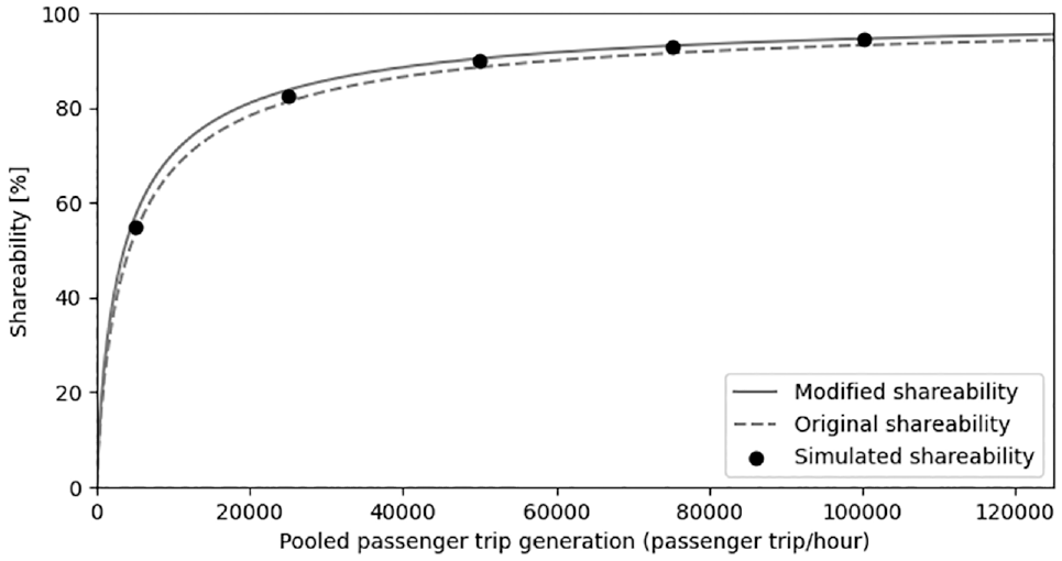
Analytical (original and modified) and simulated shareability depending on the pooled passenger trips
The dotted gray curve shows the shareability curve for the original shareability model using the constant average velocity for the base scenario
Conclusion
Summary
In this study, an analytical model to investigate the impact of ride pooling on traffic efficiency was developed by using a shareability model and the MFD for a city. A model was developed that captures the relation of average velocity and vehicle trip generation in a network, to analytically check the change in average velocity when pooling is introduced. Moreover, a modified shareability model was introduced, which derives further benefits on shareability from an improved average velocity resulting from pooling. Different scenarios were developed for a ride pooling service offered in the city of Munich, where private vehicle trips are substituted by different levels of ride pooling penetration rate ranging from 5%, to 100% (when all the private vehicle trips are substituted by ride pooling vehicle trips). The results show that this analytical model provides a very good and fast estimation of the traffic impacts of ride pooling on the urban environment, requiring only a few input data and the existence of the MFD for a city, which allows for a generalization of a model to other cities, even without the need of network simulations and calibrations, in cases when MFD is derived analytically or via empirical data ( 17 – 20 ). The analytical model is beneficial for operators to quickly assess the traffic impact of pooling in a certain area of service and for a certain sets of service quality attributes. These insights could be used in discussions with cities to allow or prioritize the operation of such a service.
Future Work
Future work will include the validation of the developed model for other cities, especially cities with higher levels of congestion in their network, where it could be possible to check if the general assumptions made for this model hold for the congestion regime as well. This would also allow further investigation into whether the assumption used for a parabolic functional form of the MFD is valid for the congestion regime, or if the functional form of the MFD needs to be adjusted to a skewed/asymmetric parabola as in Daganzo, and Laval and Castrillón ( 16 , 20 ). In addition, the validity of the parameters of the prediction model of shareability (given by Equation 4 and found by data fitting) for other cities is a topic requiring further investigation. Furthermore, the simple model used to derive the reduced number of vehicles resulting from ride pooling based on the shareability will be extended to capture analytically the impact of partially shared trips and how this depends on different optimization objectives used for the matching algorithm. Moreover, the impact of empty vehicle trips generated for passenger pick-ups or re-allocation procedures could also be investigated. The impact of induced demand from other modes, because of increased velocity as a result of ride pooling, is also an interesting topic for further consideration.
Footnotes
Acknowledgements
The authors would like to thank the anonymous reviewers, whose comments helped in improving the quality of the paper; Florian Dandl and Philipp Franeck for constructive discussions; Gabriel Tilg for sharing his expertise about the MFD; and Majid Rostami for the support with AIMSUN and the calibration of the Munich network.
Author Contributions
The authors confirm contribution to the paper as follows: study conception and design: A. Bilali, U. Fastenrath, K. Bogenberger; data collection: A. Bilali; analysis and interpretation of results: A. Bilali, U. Fastenrath, K. Bogenberger; draft manuscript preparation: A. Bilali. All authors reviewed the results and approved the final version of the manuscript.
Declaration of Conflicting Interests
The author(s) declared no potential conflicts of interest with respect to the research, authorship, and/or publication of this article.
Funding
The author(s) received no financial support for the research, authorship, and/or publication of this article.
The authors remain responsible for all findings and opinions presented in the paper.