
Abstract
Individual travel behavior, such as mode choice, is determined to a distinct degree by the respective portfolio of available mobility tools, such as the number of cars, public transit pass ownership, or a carsharing membership. However, the choice of different mobility tools is interdependent, and individuals weigh alternatives against each other. This process of parallel trade-offs is currently not reflected in typically used sequential logit models of agent-based travel demand models. This study fills this research gap by applying discrete choice and neural network models on a synthetic population to model multiple mobility tool ownership simultaneously. Using data from a national household travel survey, both model types approximated the given target distributions of mobility tools more accurately than the sequence of three corresponding logit models. Owing to its greater flexibility, the tested shallow and deep neural network exhibited higher predictive accuracy than simultaneous discrete choice models. The results indicated that neural networks with only one hidden layer were more robust and easier to formulate and interpret than deep networks with three hidden layers. Finally, the flat neural network was applied to a different synthetic population resulting in equally accurate results.
Keywords
Ownership of mobility tools, including the ownership of a car, of a public transit pass, or membership of a carsharing provider, strongly influences a person’s mobility behavior. It determines mode choice to a great extent because only if a person owns a car, for example, can he or she consider it an available mode. Therefore, to address, for example, the question of how individual motorized transport can be reduced and more environmentally friendly alternatives (public transport, sharing services, etc.) simultaneously strengthened, it is not sufficient to focus only on mode choice behavior, but also on the choice of mobility tools. Therefore, precise modeling of mobility tool ownership in travel demand models (TDMs) is essential to simulate actual mobility behavior reliably.
In research, primarily agent-based TDMs are used for this purpose. In contrast to aggregated approaches, these offer the advantage of considering individual characteristics of agents and thus mapping the interrelationships on individual mode choice decisions. Consequently, agent-based TDMs also model the ownership of mobility tools at the level of the individual. This information, in turn, influences the individual choice sets of agents in their mode choice, thus contributing to a more realistic modeling of mobility behavior.
The consideration of mobility tools in TDMs is not a new field. Internationally, car ownership, in particular, has been modeled for quite a long time, as has the ownership of public transit passes in German TDMs. In contrast, the consideration of membership models of new mobility service providers such as carsharing has received little notice in recent years. However, the current state of the art in TDMs is to model the ownership of each mobility tool separately. Consequently, the order in which individual mobility tools are modeled determines which information can be included in subsequent mobility tool ownership models. In reality, however, decisions are not necessarily made sequentially and independently of each other, but rather ownership of a car is weighed against ownership of a public transit pass, for example.
Therefore, our work aimed to develop a mobility tool ownership model that reflects the ownership of cars, the ownership of a public transit pass, and membership of a carsharing provider as a simultaneous decision. As the modeling environment, we used the agent-based TDM mobiTopp. Different modeling approaches were applied, and the models’ results were compared with each other. First, simultaneous modeling approaches were estimated based on discrete choice theory, widely used in transportation research. Second, simultaneous approaches based on machine learning (i.e., neural networks) were developed, which is a new technique in modeling mobility tool ownership.
This paper is organized as follows. First, we overview existing modeling approaches for mobility tool ownership. Second, we briefly introduce the agent-based TDM mobiTopp we applied in our study. Third, the data used for the model estimation are described. Fourth, the development of discrete choice and machine learning (ML)-based modeling approaches are explained. Consequently, the models’ results are compared, and the results of the approach with the best model fit are interpreted. Finally, we show the applicability of the selected model to a different study area and give our conclusions.
Literature Review
Car ownership models have been subject to extensive research since the 1990s ( 1 , 2 ). However, introducing mobility tools as a generic concept and modeling multiple mobility tools only emerged gradually at the turn of the millennium. From the beginning, mainly simultaneous modeling approaches of mobility tool ownership were followed. However, these were not part of agent-based TDMs.
Among the first authors who studied multiple mobility tools in a simultaneous decision model were Simma and Axhausen in 2001 (
3
). To this day, far-reaching findings on mobility tools can be traced back to their research. The authors’ study was the first to demonstrate a negative impact of car availability on public transit passes. They applied a simultaneous equation model to survey data from Switzerland, Germany, and the Netherlands. Commitment to one mobility tool significantly increased its modal use and decreased the use of other modes. Scott and Axhausen applied a bivariate ordered probit model to the number of cars and public transit passes in the household to demonstrate a substitution effect between them (
4
). Because of that substitution effect, Vovsha and Petersen emphasized that individual, closely linked mobility tools should be modeled together in one modeling step (
5
). Yamamoto concluded that for modeling bundles formed from car, motorcycle, and bicycle ownership, the structure of the multinomial logit model (MNL) could best represent bundle decisions (
6
). Similar to Beige and Axhausen (
7
) and Vovsha and Petersen (
5
), the authors had difficulties finding an adequate nesting structure. Axhausen and Beige (
7
,
8
) applied an MNL, a nested logit model (NL), a cross-nested logit model (CNL), and a multivariate probit model (MVP). The MVP applied to six mobility tool bundles better represented the interactions between these bundles through correlated error terms. The correlated error terms of bundles are highly significant, which was the authors’ justification for using the MVP and the simultaneous modeling approach. This increased explanatory potential manifested in a noticeably higher coefficient of determination,
The sequential approach is found less frequently in literature. Early researchers include Beige and Axhausen in 2004, who first applied a sequence of three MNLs to model three mobility tools (driver’s license ownership, car ownership, and transit pass ownership) sequentially ( 10 ). The influence of the exogenous mobility tool variable in the respective subsequent models was considerable. However, most transport-related TDMs consider mobility tool ownership in a sequential approach based on different discrete choice models (DCMs). Hillel et al., for example, modeled the driver’s license, number of cars per household, and public transit pass ownership with MNLs in the agent-based model SIMBA MOBi ( 11 ). However, they stated an insufficient accuracy at the regional level for modeling driver’s license ownership and the number of cars per household by the sequential logit approach., Horni et al. give additional insights into the sequential modeling procedure in the agent-based TDM MATSim ( 12 ).
Recently, there has been a trend toward using ML models to analyze individual choice decisions. Most ML models for decision modeling in transportation planning deal with the mode choice decision. For the modeling of mobility tools, only car ownership has been represented to a small extent in ML models to date. Paredes et al. compared the prediction accuracy of several ML models to that of an MNL ( 13 ). The classification task was to predict the number of cars (0, 1, and 2+). The authors emphasized the importance of preprocessing the dataset for ML models, all of which had higher predictive accuracy than the MNL tested. In ML models, depending on the type used, the rules for classifying households are said to have little to no transparency. Wang et al. compared 102 ML models and three DCMs using three datasets, three sample sizes, and three output variables (mode choice, car ownership, and trip purpose) ( 14 ). An MNL, NL, and mixed logit model were applied for the car ownership model. The top 10 ML models for car ownership had at least 11% higher accuracy than the best logit model, MNL. Therefore, Wang et al. are among several researchers advocating the increasing use of ML models in transportation modeling ( 14 ).
Axhausen and Beige were the first researchers to build bundles from mobility tools to be able to equip agents in TDMs with multiple mobility tools based on a simultaneous decision model ( 7 , 8 ). Most authors prefer this simultaneous approach in research to the sequential approach for modeling multiple mobility tools with DCMs. The variety of differently formulated DCMs proves the effort and assumptions that are necessary before modeling. However, the observable tendency toward the increased use of ML models in transportation modeling, and its lacking application in microscopic TDMs, encourage the use of ML models for the simultaneous modeling of mobility tool ownership and comparing their power with corresponding DCMs.
Agent-Based Travel Demand Model mobiTopp
For the present study, we used the open-source software mobiTopp to analyze the effects of a simultaneous mobility tool ownership model. mobiTopp is an agent-based TDM. Therefore, every person in a designated planning area is modeled as a single entity with individual characteristics ( 15 ). The travel demand simulation of each agent is based on a distinct activity program, which determines the time and duration of each activity an agent performs during the simulation period ( 16 ). The program itself is generated and executed within the framework. For the simulation period of one week, an agent chooses a destination for each activity in the corresponding activity program. Subsequently, a mode to get to the destination is chosen. For the representation of choice behavior, DCMs are applied, which guarantees autonomous, situation-dependent decision making ( 17 ).
The framework of mobiTopp consists of two modules: a long-term and a short-term module. The core of the long-term module is the generation of a synthetic population. Based on household travel survey data, households and persons or agents are generated so that aggregated statistics according to age and gender distributions, and so forth, are met. Moreover, the agents’ workplaces or locations of educational institutions are determined as fixed locations. Further characteristics of the synthetic population are modeled separately. Of particular interest in this study was the modeling of the mobility tools, which also takes place at this stage within mobiTopp. First, the number of cars per household is modeled mainly based on household characteristics. Second, a binary logit model is applied to decide whether an agent owns a public transit pass, considering sociodemographic characteristics but also, for instance, the number of cars in an agent’s household. Third, additional mobility tools, namely the membership of a carsharing, bikesharing, or e-scooter provider, are determined by distinct binary logit models. All characteristics determined in the long-term model remain fixed over the entire simulation period.
Simulation of the agents’ activity-based mobility behavior takes place in the short-term module. During the simulation period, the activity program of each agent is executed chronologically and simultaneously, and destination and mode choice models are applied. However, as only the long-term module is of interest in this study, we refer to a more detailed model description in research undertaken by Mallig et al. ( 18 ), Briem et al. ( 19 ), or Mallig and Vortisch ( 20 ).
mobiTopp has been applied successfully to several planning areas. In this study, we used the latest application of mobiTopp in the city of Hamburg, Germany, and surrounding areas. However, we focused on the city area, in which about 1.8 million persons are represented. As an indicator of the transferability of the developed approach, we also refer to the application of mobiTopp in the region of Karlsruhe, Germany, representing about 2.1 million persons.
Data
This study used data from the national household travel survey Mobility in Germany (MiD) from 2017 ( 21 ), from which 14,666 respondents could be selected for the city of Hamburg. However, because of missing responses for relevant endogenous and exogenous variables and the exclusion of individuals under the age of 14, only 6,328 observations on individuals in 4,982 different households could be used for further model development. The three mobility tools and thus dependent variables of interest were car availability, carsharing membership, and public transit pass ownership. In this study, the latter was defined as a ticket that allows users to use public transport in a specific area for at least 1 month, usually at no marginal cost, in return for a one-time payment. Owing to the design of the personal questionnaire, it was impossible to define car ownership. Instead, car availability was used based on responses to the household questionnaire. A car was considered available to a person if the household owned at least one car and the person was at least 18 years old. In our model, a person was a carsharing member when he or she reported having a membership of at least one carsharing provider. In total, 75.4% of all persons in our dataset stated that they had a car available, whereas only 15.4% were considered to be carsharing members. About a third of the respondents in Hamburg claimed to own a public transit pass.
To apply trained or estimated decision models based on the survey data to the synthetically generated population of mobiTopp, the exogenous independent variables of both datasets had to be matched. Therefore, only the survey variables that were also available for the synthetic agents could be used for training, estimation, and testing. Figure 1 provides some basic summary statistics of the sociodemographic variables for the
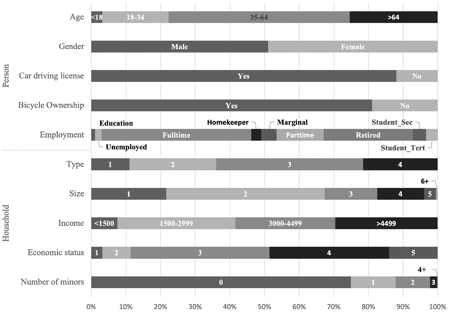
Sociodemographic characteristics used in model application.
Categorical variables were recoded into dummy variables for all models. Economic status was a calculated variable determined by the equivalized income based on household size and income.
Model Estimation
Although in research as well as in application DCMs from the field of statistics are state-of-the-art in the modeling of mobility tools, ML models have been increasingly encountered in various disciplines in recent years. Both model classes are suitable for representing individuals’ decision making and will be applied in this section to evaluate their potential to simultaneously model mobility tool ownership in TDMs. To represent simultaneity in the decision-making process and because individuals may own more than one mobility tool,
None: No mobility tool
Car: Car availability
CS: Carsharing membership
PT: Public transit pass
Car + CS: Car availability + Carsharing membership
Car + PT: Car availability + Public transit pass
CS + PT: Carsharing membership + Public transit pass
All three: Car availability + Carsharing membership + Public transit pass
Discrete Choice Models
Discrete choice theory goes back to McFadden ( 22 , 23 ) and was further developed by Ben-Akiva ( 24 ), among others. From this class of models, the widespread MNL, NL, and CNL were applied to the modeling object of this study, using the Apollo package in R for implementation ( 25 ). For all three DCMs, the eight defined bundles of mobility tools represented mutually exclusive and collectively exhaustive choice alternatives. Despite the several advantages of the MNL model, such as its theoretical soundness and mathematically simple and comprehensible analytical structure, the main concern of the MNL remained the potential violation of the independence from irrelevant alternatives (IIA) property. The IIA property was not likely to be valid as some mobility tool bundles were closer substitutes than others. Allowing for correlations between the utilities of alternatives in common nests, the NL and CNL models have been suggested and widely established ( 24 , 26 , 27 ). In an exploratory approach, an expedient nest structure with the three nests “Car, Car + CS,”“Car + PT, All” and “CS, PT, and CS + PT” was identified for the NL.
Contrary to several other nest structures, this structure yielded reasonable nest coefficients and a satisfactory approximation of the actual benchmarks of the mobility tools. In the CNL, the bundles with only one mobility tool were located on the first level. On the next level, combined mobility tool bundles were connected to the higher-level nests if the bundle contained the depicted mobility tool of the nest. Since bundles belonged to multiple nests in the CNL, this model could model a more flexible correlation structure than the NL. Figure 2 illustrates the structure of both models and presents a summary of relevant statistics.
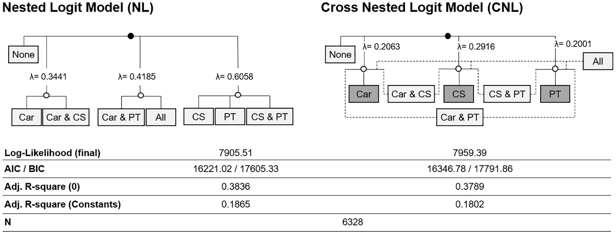
Structure and main results of estimated discrete choice models.
In the DCMs, all numeric and categorical variables were dummy-coded. Table 1 shows how many dependent variables were included in the utility functions of the different simultaneous models and the sequential submodels. For the simultaneous DCM, the number of dummy-coded variables differed from bundle to bundle. Similarly, a different number of variables were used in the multiple utility functions of the sequential model. For details on the car ownership model as part of the sequential DCM, we refer interested readers to Barthelmes et al. ( 28 ).
Overview of the Dependent Variables in the DCMs
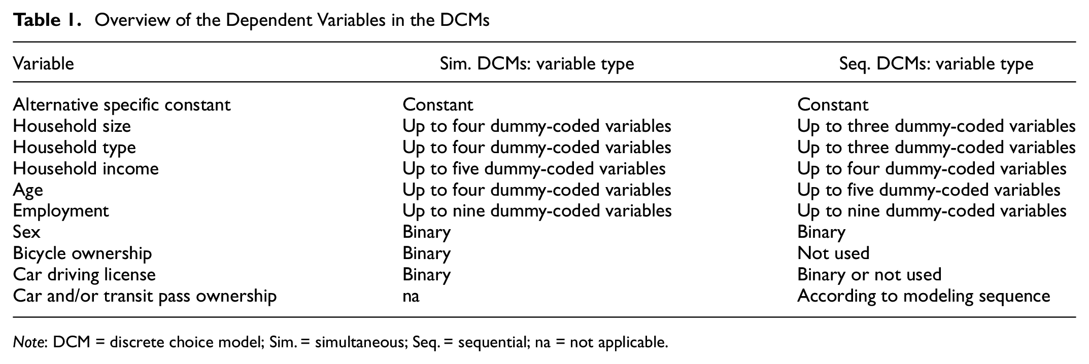
Note: DCM = discrete choice model; Sim. = simultaneous; Seq. = sequential; na = not applicable.
Neural Networks
Neural networks (NNs) are an ML method from artificial intelligence. These mimic the physiology and functioning of the human brain. The aim is to simulate how “the human brain processes information” ( 29 ), which is why NNs are suitable for reproducing the decisions of real people for artificially generated agents. In recent years, a steady increase in ML concepts for decision analysis has been observed in several fields, including business, biology, and transportation.
In the transportation sector, ML models are increasingly challenging the McFadden-based class of DCMs. In research, both approaches are applied to individual decisions and compared with respect to several criteria, for example, predictive accuracy, interpretability, and robustness (14, 30–32). ML models achieve their superiority over DCMs in particular owing to the low preprocessing effort, no structural assumptions being necessary, no nest structure requiring specification in advance, the consideration of nonlinearities, and the inclusion of all, and thus also correlated, variables as inputs. Therefore, users do not need expertise, domain-specific knowledge, or experience to specify a decision model with utility functions. Owing to this high flexibility and predictive power, the class of ML models represents a legitimate alternative to DCMs to model the decision of mobility tool ownership simultaneously.
To balance overfitting and underfitting, complex problems require complex models and simple problems require simple models. According to the universal approximation theorem, an NN with only one hidden layer containing a finite number of neurons can approximate any continuous function with reasonable accuracy, whereas more complex NNs are used in various applications today ( 33 , 34 ). Since ML models have not been applied to multiple mobility tools to date, two extremes of NNs with respect to the complexity of the network structure were applied to the modeling object: a simple shallow NN (SNN) and a wide, deep NN (DNN).
The SNN was implemented using the CARET package in R, and the DNN using the advanced keras package ( 35 , 36 ). Both the SNN and the DNN had 21 neurons in their input layer and eight neurons in their output layer, representing the eight bundles of mobility tools. The SNN, as shown in Figure 3, had one hidden layer with 24 neurons.
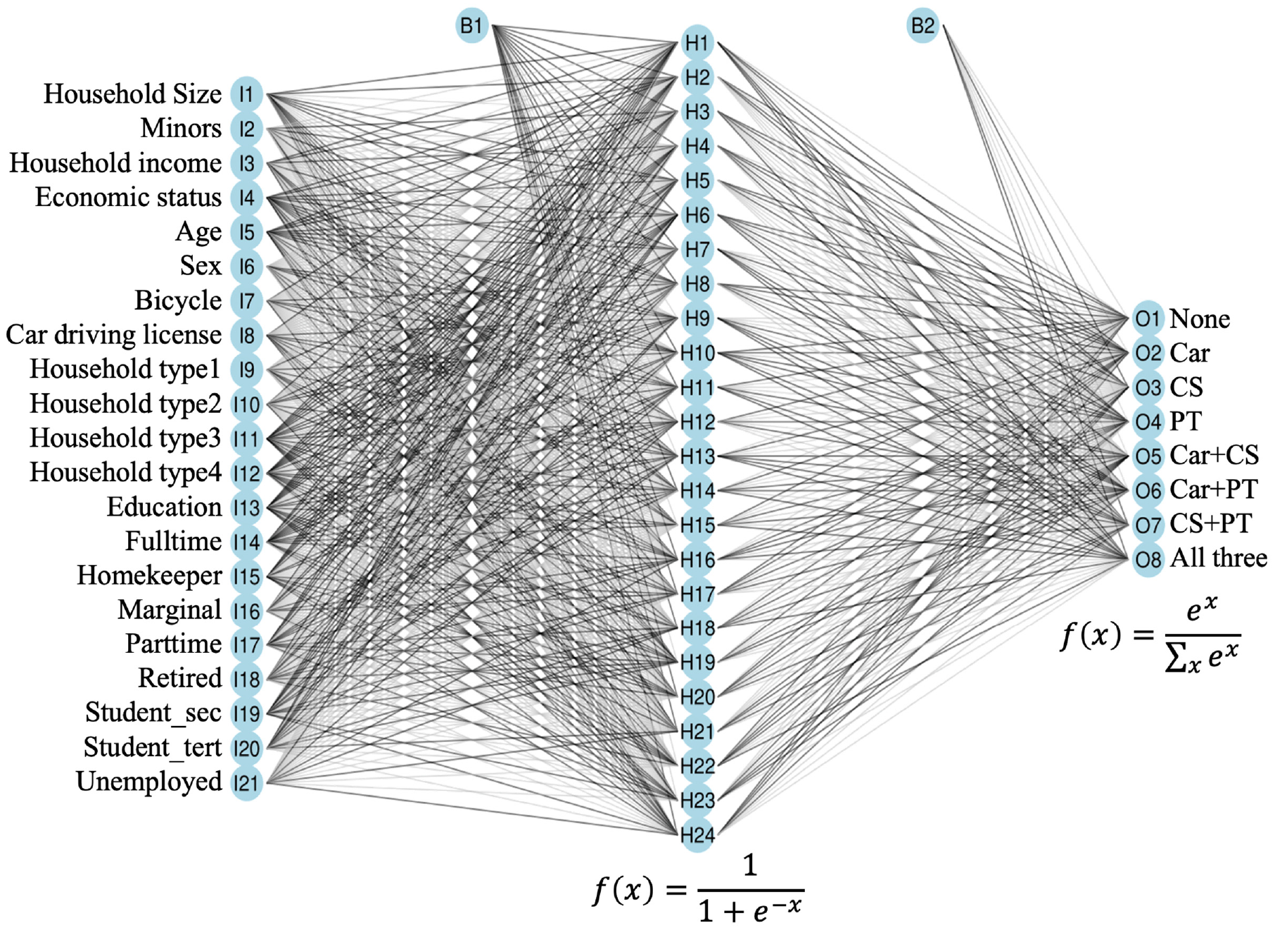
Shallow neural network of mobility tool bundle ownership.
This number resulted from an exploratory analysis of different widths of the network. Twenty-four neurons in the hidden layer achieved the slightest deviations on the test dataset concerning cross-validation and meeting the target distribution of mobility tool bundles after application to the synthetic population. In a similar approach, layer widths of 100, 80, and 60 were determined for the three hidden layers of the DNN. Additionally, dropout rates of 0, 0.2, and 0.3 were tested and applied to layers of the DNN. To incorporate nonlinearity, the activation function used in the hidden layer in the SNN was the logistic sigmoid function, and the rectified linear unit function (ReLU) in the DNN. The latter was used in the DNN to prevent the problem of vanishing gradients. Combinations of the ReLU function required the hidden layers of the DNN to consist of a higher number of neurons.
The softmax function represented the activation function of the output layers of both networks. As shown on the right in Figure 3, the softmax function was applied to calculate probabilities in output layers of classification problems with more than two labels. The cross-entropy function was used as a loss function. It measured the performance of a classification model whose outputs were probability values between 0 and 1. Combining this loss function with the softmax activation function in the output layer has the advantage that the output values of an NN can be interpreted as probabilities. Moreover, the value of the cross-entropy loss function can be interpreted as a negative log-likelihood value. Thus, the log-likelihood value of a DCM can be compared with the value of the cross-entropy loss function in an NN. The loss function of the converged SNN had a significantly lower loss function value of 7,279.35 than the best logit model, the NL, with a value of 7,905.51. This higher model goodness of fit to the data can be attributed to the flexible modeling capabilities of the NN.
The stochastic gradient method is an optimization algorithm to minimize the cross-entropy function. Further development of the gradient method, the “Adam” optimization algorithm, showed a slightly higher deviation from the target distributions with otherwise identical hyperparameters. The backpropagation method minimizes the cross-entropy loss function by adjusting the weights. Using this gradient descent procedure, the weights from the last to the first layer were optimized to minimize the difference between the calculated output of the NN and the correct label. These processes enabled learning in the true sense. For the SNN, the learning rate and the decay parameter were set to default values. For the more complex DNN, additional hyperparameters could be set in the package used, primarily to accurately approximate the given target distribution of the household survey MiD used.
Finally, from the eight probabilities calculated by the NNs, a bundle of mobility tools was assigned to each of the over 1.6 million agents older than 14 years. The calculated probabilities formed the base for a cumulative distribution function, in which a mobility tool bundle with a higher probability covered a greater proportion of the function’s definition span between 0 and 1. Afterwards a random number was drawn between 0 and 1, the same range as the distribution function. Based on the random number the distinct mobility tool bundle was assigned. The same procedure was also applied for the DCMs.
Results and Discussion
In this section, we will first compare the goodness of fit of the previously presented models with regard to their accuracy in modeling mobility tool ownership. Second, further insights into the interpretation of the SNN are given. Finally, we apply the ML model to a different study area and analyze the results.
Comparison of Models’ Goodness of Fit
The models were assessed by comparing the deviation of the distribution of the predicted mobility tool bundles of the synthetic population of Hamburg from the given target distribution based on the reported characteristics in MiD 2017 of Hamburg’s citizens. Key results of this comparison are presented in Table 2. The last row represents the benchmark or true distribution against which the models were tested. According to the sequential logit, the results of the calibrated and the uncalibrated model are presented. Although the latter refers to the raw estimated logit, in the calibrated approach, the model’s parameters were adapted to meet the distribution of the three single mobility tools—Car, CS, and PT—not only overall but also in meeting the distributions of incorporated influencing factors such as age and gender. The calibration was also done sequentially for each of the mentioned mobility tools.
Model Comparison with respect to Target Mobility Tool Distributions for Hamburg
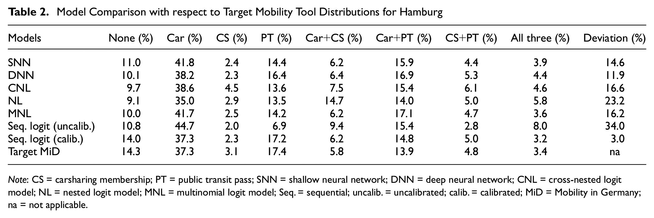
Note: CS = carsharing membership; PT = public transit pass; SNN = shallow neural network; DNN = deep neural network; CNL = cross-nested logit model; NL = nested logit model; MNL = multinomial logit model; Seq. = sequential; uncalib. = uncalibrated; calib. = calibrated; MiD = Mobility in Germany; na = not applicable.
The two models developed in this work that most accurately approximated the target distribution of the MiD were the DNN and the SNN. The summed deviations were 11.9% and 14.6%, respectively. All three simultaneous logit models performed differently. However, all of them underestimated the proportion of agents without mobility tools and with public transit passes. Although the MNL and CNL had slightly higher deviations than the SNN, the predicted probabilities of the NL had a comparatively high inaccuracy of 23.2%. It was to be expected that a simultaneous modeling approach would outperform an uncalibrated, sequential model. However, the high deviations of the existing sequential logit model in the uncalibrated version, which resulted from the maximum likelihood estimation procedure, were striking. The exceptionally high share of car availability and low share of public transit pass ownership in the uncalibrated sequential logit model may be related to the modeling order: in the first step, car ownership was modeled at the household level, which had a significant negative impact on public transport pass at the second modeling level. Only by calibration does the sequential logit model achieve an accuracy exceeding the simultaneous models. However, this manual intervention requires substantial effort. The availability of reliable target distributions is mandatory, and it aligns a model to a specific case, which may restrict its applicability in another (regional) context. For both NNs, the best effort was put into estimation and validation, but no further calibration was performed for the NNs or for the simultaneous DCMs. Therefore, those models should be compared in the first instance with the uncalibrated sequential logit model. All developed models underestimated the proportion of agents without mobility tools and overestimated the proportion of agents with car availability, except for the overall inaccurate NL. This overestimation may be related to the definition of car availability as a mobility tool.
Table 3 shows the accuracy of selected models for the most striking sociodemographic characteristics. The accuracy rates represent the deviation of the models—applied to mobiTopp’s synthetic population—in comparison to the target values of the MiD for the distribution of the selected sociodemographic variables. In this sense, 0.00% would represent a perfect fit for the corresponding distribution of a sociodemographic characteristic. The deviations presented are averaged over all mobility bundles.
Model Comparison Concerning Agents’ Age, Sex, and Household Income
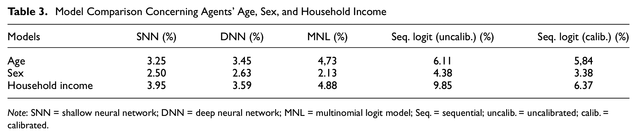
Note: SNN = shallow neural network; DNN = deep neural network; MNL = multinomial logit model; Seq. = sequential; uncalib. = uncalibrated; calib. = calibrated.
An analysis of the variables presented and the remaining variables argued for the predictive accuracy of NNs. The SNN most accurately approximated the target distributions of sociodemographic characteristics of the eight mobility tool bundles across all characteristics. The MNL, as the most accurate simultaneous DCM, had, on average, an insignificantly lower precision than the SNN. The uncalibrated logit model clearly missed the target distributions within the eight mobility tool classes for the displayed sociodemographic characteristics, as well as on average. Although the calibrated sequential model obtained the best overall accuracy according to the target distribution of all mobility tool bundles, Table 3 shows that the calibrated model was lacking in meeting the structural sociodemographic patterns within each mobility tool bundle. Therefore, no significantly higher accuracy was achieved by calibration. These still high deviations indicated inconsistency within the mobility tool classes. In an agent-based model, the most striking benefit is to be able to depict such structural differences, which the current calibrated logit model seemed to do worse than the simultaneous approaches, specifically the NNs. Furthermore, during the calibration process, a lot of effort was made to align the model with the overall target distributions of all mobility tool bundles, also respecting the sociodemographic characteristics within a mobility tool, as described before. For the simultaneous approaches, this effort was not made. Nonetheless, the models showed significantly better results, leading to the assumption that simultaneous modeling of mobility tool ownership may better reflect sociodemographic patterns even though the overall accuracy may be lower.
In summary, the NNs outperformed the simultaneous DCMs and the sequential logit model and exhibited high sociodemographic consistency within mobility tool bundles. Although the DNN had a slightly higher accuracy than the SNN, its disadvantages as a more complex model included the increased effort required to find an adequate combination of hyperparameters for the given problem, the observed high sensitivity to changing hyperparameters, and the tendency toward overfitting ( 14 , 37 ). The SNN exhibited greater robustness to changes in the number of neurons, more straightforward interpretability, and a low risk of overfitting. As a simply constructed network, it was suitable for the comparatively simple classification task in our study. However, were the complexity to increase by adding hidden layers, combining neurons with nonlinear activation functions across multiple hidden layers would lead to models that could not be evaluated with a mathematical formula. For the sequential logit model, extensive calibration of the model was necessary. However, within the eight mobility tool bundles, there were still significant inconsistencies with MiD’s sociodemographic control variables in the sequential DCM. Therefore, the validity of the hierarchical approach of the sequential logit, which considered causal relationships between mobility tools in only one direction, was questionable, as the order in which each mobility tool was modeled influenced the information that could be used in subsequent mobility tool models. Simultaneous models differently consider causal interactions between mobility tools in both directions: all mobility tools can influence each other because the decision on all mobility tool bundles is taken at the same time in one model, reflecting each other’s dependencies.
According to Janiesch et al., for the selection of the appropriate model, several factors, not solely the models’ accuracy, have to be considered ( 37 ). Based on the overall accuracy, the DNN performed best, followed by the SNN, and then the simultaneous MNL. Considering the advantages of the SNN over the DNN in our study, as described before, we decided to favor the SNN as the model with the second-best performance in the course of our study. Although the simultaneous MNL was a simpler model, its performance was worse than the SNN.
Interpretation of Results of the NN
The interpretability of NNs is highly relevant for control, transparency, trust, and the generation of new knowledge. In DCMs, coefficients provide information about an attribute’s influence on an alternative’s utility. In NNs, coefficients cannot be read off, and the processes within a network remain hidden from the user, which is why complex NNs, in particular, are considered to be “black boxes” (
30
,
38
). Consequently, numerous methods have been developed in recent years to open the black box of an NN. Accumulated local effect (ALE) plots represent a modification and further development of the widely applied “partial dependence plots.” They overcome the strict assumption of partial dependence plots, in which features must be uncorrelated. Moreover, they are much less computationally intensive. An ALE plot calculates the change in a class’s prediction at a location,
In the following, the ALE plots of the significant, meaningful features in the SNN are analyzed. The methods of permutation feature importance ( 39 ) and that of Olden ( 40 ) showed the importance of the variable “age” in the SNN. Figure 4 reveals that from the age of 75, the probability of not owning a mobility tool rose. The probability of only having a car available in the household increased sharply with age. The “PT” and “Car + PT” bundles were relatively independent of age, which was consistent with previous findings. For young adults, the likelihood of having a carsharing membership increased. From the age of about 50, this characteristic had a negative impact on bundles containing carsharing membership.
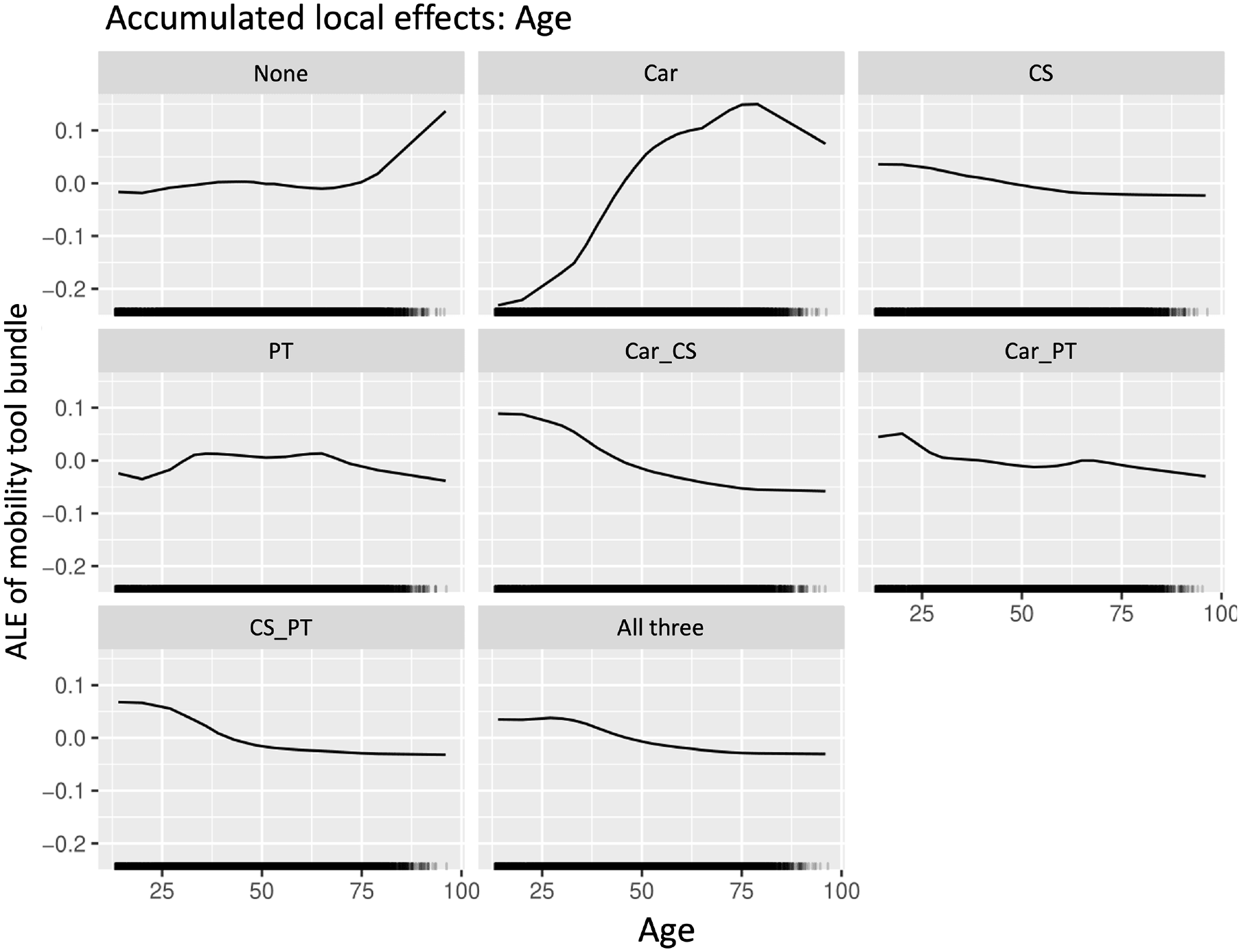
Accumulated local effect plot for variable “age.”
In addition to age, household income had a significant impact on the provision of mobility tools, as its high values of the feature importance methods suggest. The ALE plots of this variable showed reasonable effects, as presented in Figure 5. For households with a monthly income lower than around €2,500 (€1 = $1.13; year of reference: 2017), the probability of not having a mobility tool increased. The probability of having only a car available increased for persons with a household income up to about €2,500, whereas the probability slightly reduced for higher incomes. The probability of having a complementary carsharing membership in addition to a car available followed a monotonous increasing curve with a positive probability contribution of primarily wealthy households with a monthly income exceeding around €4,000. A combination of car availability and public transit pass ownership tended to be observed increasingly among households with incomes between €2,500‚ and €7,500. For households below this range, the probability was reduced. In lower income ranges, the probability of owning only a public transit pass increased. It can be seen that persons in higher-income households tended to supplement an available car with personal mobility tools.
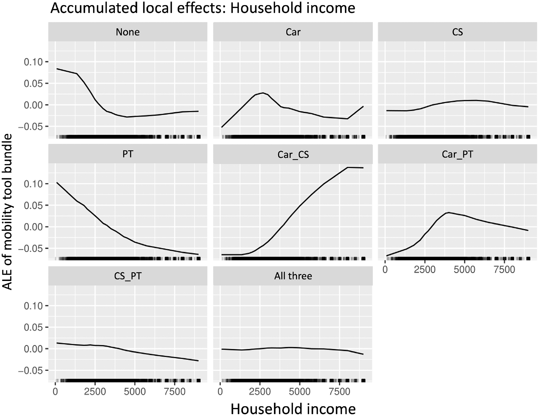
Accumulated local effect plot of variable household income.
Household size must also be considered when analyzing household income. The influence of not owning a mobility tool was negative and fell steadily to −15% for households with three persons or more compared with the average prediction. People in households with at least three members increasingly chose the “Car + PT” bundle at an above-average rate. The “Car” bundle experienced a significant increase in utility for individuals in two-person households to more than 10% above the average prediction for this bundle. Unsurprisingly, exclusive carsharing membership became less attractive for larger households. This was similarly true for the “PT” bundle, which had an increased probability for a one-person household.
The ALEs of these variables and those not presented here were consistent with the results of previous research and considerations of behavioral theory. Although the interpretability was not at the level of a DCM, the ALE plots increased the interpretability of the NNs. Also, pointing out nonlinearities could help users to judge inputs’ meaningfulness and plausibility.
Application of the Developed Method to a Different Area
The question arises as to what extent the methodology used could achieve comparably good results in other study areas and under different framework conditions, or whether the NN methodology was too strongly tailored to the data of Hamburg. This investigation was an important feature and prerequisite to confirm the results of the approach.
After the NNs had achieved precise and consistent results for the city of Hamburg, an NN was transferred to the synthetic population of the mobiTopp application in the metropolitan area of Karlsruhe, Germany, by retraining the SNN. Only the SNN was applied, as this model performed better than the other simultaneous approaches and confirmed with with a lower risk of overfitting and greater robustness than the DNN. DCMs were not considered as they had a worse overall performance for the Hamburg model, and were also less capable of precisely reflecting sociodemographic characteristics in the mobility tool ownership decision as presented in Table 3. Owing to restrictions in the regional aggregation level of the previously used MiD dataset, a different MiD dataset with less detailed sociodemographic information had to be used to restrict the dataset to being as close as possible to the planning area of the Karlsruhe model. Thus, a new training and testing dataset was used for the SNN. Compared with Hamburg, the modeled area contained more rural regions, leading to a different, more unbalanced distribution of mobility tool bundles. The SNN was trained with a population of an area that included 1.76 million inhabitants in reality, whereas the population of the modeling area in mobiTopp was 2.09 million agents. The available sociodemographic variables differed from those in the Hamburg model because of restrictions in the level of detail in the used dataset. Instead of using 21 inputs, the SNN in the Karlsruhe model learned relationships using values from 16 inputs. Adapted to the SNN of the Karlsruhe model, 19 neurons were used in the hidden layer, again three more neurons than the number of inputs. They again showed the slightest deviations from the target distribution. The robustness of the SNN’s predictive ability for mobility tool bundles against different widths of the SNN was repeatedly observed as changes in the hyperparameters of the SNN provided only a small variation in its predictive ability. The explanatory power of the SNN was also diminished by the smaller MiD dataset of 2,517 observations in the region of Karlsruhe. Nonetheless, compared with previous studies that applied ML models in transport modeling, the training data size was considered sufficiently large for both Hamburg and Karlsruhe. In the meta dataset presented by Wang et al., most studies used sample sizes between 1,000 and 10,000 ( 14 ). Consequently, the SNN was trained using a smaller, more unbalanced dataset with a smaller number of inputs that covered more than 1.76 million people at the end of 2020. However, mobility tools were assigned to 2.09 million agents, and the network was evaluated using the MiD target distribution of the area projected to cover 1.73 million people in 2017.
Table 4 shows the distributions of the SNN and the uncalibrated sequential logit model compared with the target distribution of the MiD for the mobiTopp model in Karlsruhe. In addition, the distribution of mobility tool bundles within the training dataset is shown in the lower table, which was used to train the SNN. As previously stated, neither a DNN nor simultaneous DCM were applied and are therefore not presented.
Model Comparison with respect to Target Mobility Tool Distributions for Karlsruhe
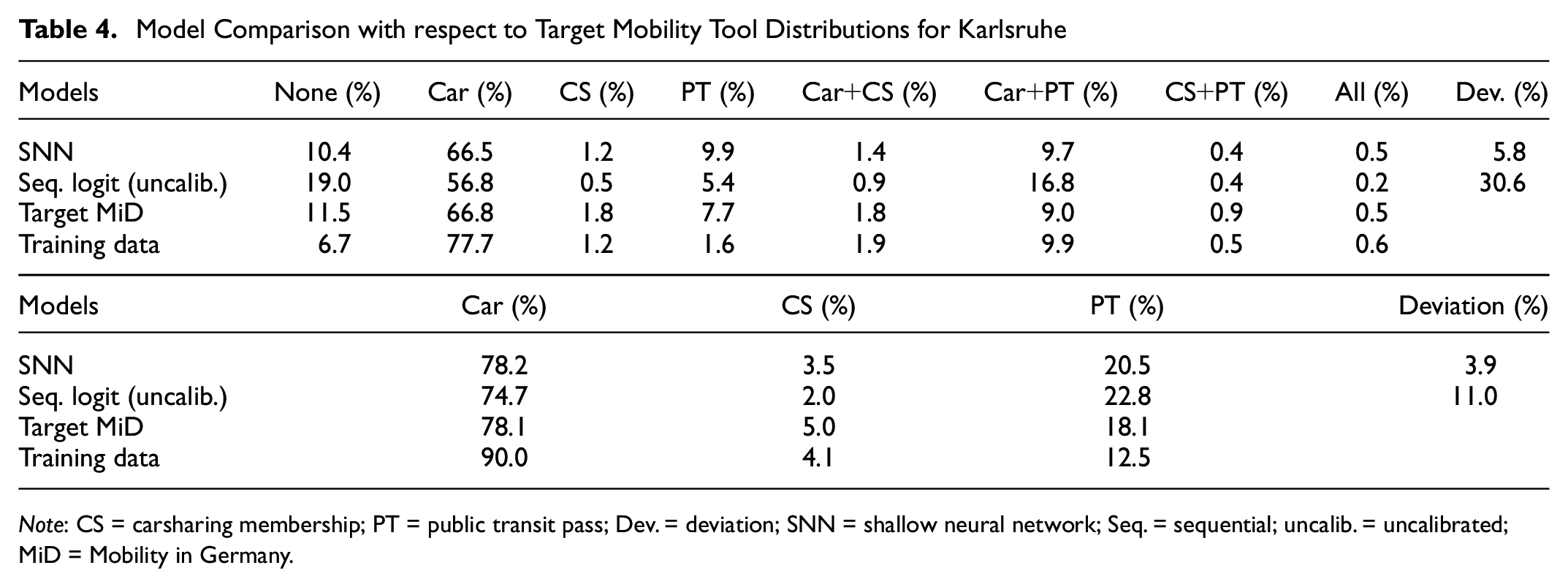
Note: CS = carsharing membership; PT = public transit pass; Dev. = deviation; SNN = shallow neural network; Seq. = sequential; uncalib. = uncalibrated; MiD = Mobility in Germany.
Primarily, it should be emphasized that the SNN again showed a much higher prediction accuracy than the uncalibrated sequential logit model. That the modeling area was based on the target distributions was not congruent with the modeling area of the SNN and that the target distributions were not to be considered exactly could mitigate some of this discrepancy. Nevertheless, the observable deviations of the logit model were similar to those of the Hamburg model and were considerable. Unlike in the Hamburg model, the highest summed deviation resulted mainly from the overestimation of the bundles “None” and “Car + PT” and the underestimation of the “Car” bundle. The logit model predicted the target distributions of mobility tools at the individual level more precisely than in the Hamburg model. Car availability was below the MiD control variables, and public transit pass ownership was above. This was oppositely observed in the Hamburg model. With a deviation of 5.8%, the SNN’s overall accuracy was above its equivalent model of the Hamburg area, where the deviation was 14.6%. In absolute terms, the most substantial variations were observable for public transit passes and people without mobility tools. In contrast to the Hamburg model, car availability was predicted at the individual mobility tool level with high accuracy.
In summary, it can be said that the SNN also achieved high prediction accuracy for regions other than Hamburg. For the synthetically generated population of the mobiTopp model of Karlsruhe, the MiD target distributions were also approximated accurately. In contrast, the sequential logit model was far less precise owing to serial maximum likelihood methods. In the SNN, the changed framework conditions of the smaller, less balanced dataset with a smaller number of inputs or more aggregated information did not harm the precision of the results. The effort in applying the SNN to other study areas was primarily in matching the variables of the training dataset with the variables of the agents of the synthetic population. Based on this, the number of neurons in the hidden layer of the SNN must be adjusted, as well as the number of iterations, depending on the size of the training dataset.
In addition, for transport policy makers as well as transport researchers, it is not only of interest which model best reflects the status quo but also how it might be used for the forecasting and evaluation of certain mobility scenarios. This could include, among other factors, the consideration of an additional mobility tool, but also the (politically influenced) change in the attractiveness of certain mobility tools. The simultaneous approach results in an exponential growth of complexity, with each additional mobility tool to be considered owing to the combinatorial problem of building mobility bundles. However, a researcher has to specify an exponentially increasing number of utility functions when using DCMs, whereas, for ML models, this effort can be neglected as only the number of variables in the output layer increases exponentially. In contrast, DCMs are more suitable, for instance, for reflecting changes in the attractiveness of certain mobility tools. In DCMs, parameters can easily be manipulated, and therefore certain influences for a future mobility scenario could be considered. Such a direct intervention is not possible for ML models. Both aspects have to be considered—in addition to accuracy—by a modeler when analyzing mobility tool ownership and be weighed and evaluated in the choice of model type depending on the study’s objective.
Conclusion
In existing TDMs, mobility tool ownership is typically modeled in sequential DCMs. However, literature has already found evidence that a simultaneous modeling approach reflects the decision process more comprehensively. In the present study, we were able to reveal relevant insights. Integrating a simultaneous mobility tool ownership model (i.e., car availability, public transit pass ownership, carsharing membership) showed greater potential to more accurately reflect structural sociodemographic patterns of mobility tool ownership in TDMs than sequential approaches. Applying ML models offered tremendous potential to further improve the simultaneous simulation of mobility tool ownership in TDMs compared with uncalibrated DCMs—we showed a generally higher overall prediction accuracy according to the target distribution.
In addition, using the example of a synthetic population in the city of Hamburg we demonstrated that, according to the model’s results and the effort involved in building the model, NNs were superior in accuracy and flexibility to simultaneous nested logit or cross-nested approaches. However, when applying an NN approach to model mobility tool ownership, we found SNNs easier to build and handle and more robust than DNNs. Moreover, we have shown that retraining an NN to a different study area also resulted in accurate modeling of mobility tool ownership, and the effort of estimating a new DCM from scratch can be avoided if the structure of the new dataset is the same as in the initial model.
However, all these results were based on the comparison of NNs with uncalibrated DCMs. Our study also showed that the slightest deviation from a target distribution of mobility tools was achieved for a calibrated, sequential DCM, which emphasized the power of the possibility of calibrating DCMs. However, our study also showed that even the calibrated model was less capable of reflecting sociodemographic patterns between the different mobility tool bundles than all estimated simultaneous models. Consequently, when simultaneously modeling mobility tool ownership in a TDM, a researcher must weigh the possibility, but also the consequences, of calibrating DCMs against the flexibility and robustness of NNs. Moreover, our study focused mainly on the models’ performance in relation to accuracy. From a practitioner’s perspective other aspects, such as the models’ applicability and transferability to future mobility scenarios, are also of importance. However, each of these aspects must be weighed individually by each user according to his or her study’s objective—our study has provided the necessary quantitative background on the models’ accuracy performance.
In our study, even when applying the model to another study area, we used the same data based on the German household travel survey, MiD. In a further application, we need to test the robustness of both modeling approaches with a different database. We additionally intend to specify the tested DCMs in the Hamburg model for the Karlsruhe model to further support our results. Moreover, we need to compare the ML approaches with more complex DCMs, such as a mixed logit and a multivariate probit model. As our study has shown the benefits of ML approaches and DCMs, we are considering applying hybrid models in the next step, combining the advantages of both models. Apart from those technical issues, we also need to reflect on the effects of the different modeling results on actual mode choice behavior.
Footnotes
Author Contributions
The authors confirm contribution to the paper as follows: study conception and design: J. Püschel, L. Barthelmes, M. Kagerbauer, P. Vortisch; data collection: J. Püschel, L. Barthelmes; analysis and interpretation of results: J. Püschel, L. Barthelmes; draft manuscript preparation: J. Püschel, L. Barthelmes. All authors reviewed the results and approved the final version of the manuscript.
Declaration of Conflicting Interests
The authors declared no potential conflicts of interest with respect to the research, authorship, and/or publication of this article.
Funding
The authors received no financial support for the research, authorship, and/or publication of this article.
Data Accessibility Statement
The datasets used in this research are available from the Traffic Clearinghouse at the German Aerospace Center (DLR).