
Abstract
The interaction between mixed autonomy traffic and public transport vehicles competing for limited road space is a less explored area of research. To evaluate the traffic dynamics in bimodal networks, a three-dimensional (passenger) network fundamental diagram, known as 3D-NFD (3D-pNFD), can be estimated that relates the accumulation of cars (autonomous and human-driven) and buses to the network vehicular (passenger) travel production. In this study, we propose a 3D-pNFD-based congestion pricing scheme considering three vehicle classes of buses, system-optimal (SO) seeking connected and automated vehicles (CAVs), and user-equilibrium (UE) seeking human-driven vehicles (HVs). We develop an iterative tri-level modeling framework for mode choice, pricing, and route choice in a mixed autonomy network. The lower level generates mixed equilibrium traffic flow through an integrated mixed equilibrium simulation-based dynamic traffic assignment model and a transit assignment model. The mid-level finds the optimal toll rates through a 3D-pNFD feedback-based controller. A nested logit-based mode choice model is also applied to capture travelers’ preferences toward three available modes and incorporates elastic demand. To encourage CAVs to follow the SO routing mode, they are provided with a discount on the congestion toll whereas UE-seeking HVs are subject to full price toll. Buses are also entirely exempt from the toll. We explore three scenarios with different discount rates on SO-seeking CAVs to investigate the effect of the incentive plans on the mode choice behaviors of road users in the pricing zone. The performance of the proposed model is evaluated in a large-scale network in Melbourne, Australia.
Connected and automated vehicles (CAVs) are expected to change the way people travel in future cities. Several studies in the past have already evaluated the potential impacts of CAVs on traffic flow and people’s travel choices in mixed autonomy networks. Traffic safety, mobility, accessibility, signal controlling, and parking management are also expected to be improved when CAVs are more widely adopted ( 1 – 6 ). Given Vehicle-to-everything (V2X) technologies enabling CAVs to communicate with other vehicles as well as a central agent, they can be leveraged as mobile actuators to regulate traffic flow and reduce congestion. This enables CAVs to follow the system-optimal (SO) routing principle to reduce the inefficient behavior of the user-equilibrium (UE)-seeking human-driven vehicles (HVs) ( 7 – 10 ). On the other hand, CAVs’ potentially higher levels of comfort and accessibility compared with the other modes raise a concern that they may increase the public willingness to use CAVs, thus causing induced demand and traffic congestion in the network. Congestion pricing is a commonly used scheme to alleviate the impact of potential traffic congestion and incentivize sustainable travel modes like public transit.
The classical approach for determining the toll rates is based on economic theories and has been significantly developed over the years (for a comprehensive review, see Yang and Huang [ 11 ] and De Palma and Lindsey [ 12 ]). However, the classical approach often fails to support practical developments for network-level congestion pricing ( 13 ). The traffic models applied in econometric models use link travel cost functions that assume a steady-state traffic condition. Thus, they do not often accurately replicate the traffic dynamics and fail to relate with network-level characteristics. Such approaches usually overlook the temporal aspect of congestion propagation in the system and consider it as memory-less individual functions of demand at a given time ( 14 ). Also, pricing individual links in a network is difficult to implement in practice, and finding the optimal toll is computationally expensive in large-scale networks ( 15 ). To overcome these challenges, network-level traffic dynamic models have been applied that are computationally tractable and consistent with the physical properties of traffic. Network-level macroscopic modeling of urban networks has caught significant attention since the empirical confirmation of the existence of network fundamental diagram (NFD) or macroscopic fundamental diagram (MFD) by Geroliminis and Daganzo ( 16 ). NFD or MFD represents the relationship between traffic flow and density at the macroscopic scale that has been applied in various perimeter control and congestion pricing studies ( 10 , 17–21). However, traffic flow is multimodal in the real world and the interactions between different travel modes competing for the road space need to be considered. To evaluate traffic dynamics in bimodal networks, a three-dimensional (3D)-NFD was first introduced by Geroliminis et al. ( 22 ); it relates the accumulation of cars and buses to the network vehicular flow. The first empirical 3D-NFD and 3D passenger NFD (3D-pNFD) were estimated by Loder et al. ( 23 ) for the city of Zurich, Switzerland, to capture the interactions between cars and public transport from both vehicle and passenger perspectives. They used empirical data from loop detectors and automatic vehicle location devices of the public transportation vehicles and proposed a statistical model to predict the effects of vehicle accumulation on the speed of cars and public transportation vehicles. The authors estimated 3D-NFDs (3D-pNFDs) in which the network travel production (network passenger production) was illustrated as a function of the accumulation of cars and public transportation vehicles.
To the best of our knowledge, integrating the transport network multimodality into NFD-based pricing has not been studied before and, thus, offers new contributions to the literature. In this study, we develop a tri-level model for joint routing and pricing control in bimodal mixed autonomy networks with elastic demand using the concept of 3D-pNFD, building on the previously published modeling framework by Mansourianfar et al. ( 10 ). The developed framework in this study includes a nested logit mode choice model to capture travelers’ preferences toward three available alternatives: automated vehicle (AV), HV, and bus. In a congested network, SO-seeking CAVs whose routing is being controlled centrally may have to take longer routes. In return, to encourage CAV owners to stick to the SO routing, they are provided with a discount on the congestion toll. Mansourianfar et al. ( 10 ) have argued that providing a full toll exemption for the SO-seeking CAVs entering a pricing zone can considerably increase the optimal toll rate imposed on the remaining UE-seeking HVs to keep the pricing area uncongested. They showed that widespread adoption of SO-seeking CAVs (beyond 60%) would impair the effectiveness of the incentive-based pricing scheme because the number of SO-seeking CAVs in the pricing zone would increase significantly, and even imposing high tolls on the remainder of UE users cannot keep the pricing zone uncongested. Introducing two different toll rates could solve the issue. Imposing tolls on SO-seeking CAVs could also make public transportation a more attractive alternative for some travelers.
The present study extends the study by Mansourianfar et al. ( 10 ) and incorporates a transit assignment model into a previously developed mixed equilibrium simulation-based dynamic traffic assignment (SBDTA) model. It also incorporates a mode choice to relax the inelastic demand assumption and to find the modal split endogenously. To control the traffic dynamics in the bimodal network, a 3D-pNFD is estimated and incorporated in the proposed congestion pricing model to optimize the passenger flow and keep the central business district (CBD) uncongested for both modes. A toll rate is dynamically optimized and imposed on the UE-seeking HVs, whereas a discount rate on the congestion charge is applied for SO-seeking CAVs entering the pricing zone. We explore three scenarios with different discount rates on SO-seeking CAVs to investigate the effect of incentive plans on traffic patterns. Given the determined toll rates, the generalized costs and probabilities of selecting each mode are estimated and fed back to the integrated mixed equilibrium SBDTA and transit assignment model. This process continues iteratively until an equilibrium point in the system is found. Although buses often make up a small share of road traffic compared with private cars, their high passenger occupancy underscores the need for prioritization. This priority, coupled with the proposed pricing on private vehicles, can reduce overall congestion in the network, providing more space to public transport within the pricing zone. In this study, we do not aim to examine the mesoscopic or microscopic interaction dynamics of buses in mixed autonomy traffic. The assumption is that buses interact with the rest of the traffic similar to an HV.
The developed methodology is comprehensively described in the next section in which we explain the applied mode choice model, 3D-pNFD-based congestion pricing controller, and the integrated mixed equilibrium SBDTA and transit assignment model. In the section on numerical experiments, we demonstrate the performance of the proposed framework on a subnetwork of Melbourne, Australia. We estimate the 3D-NFD and 3D-pNFD of the bimodal network using simulation data and statistical models that are applied to the pricing model. We then determine the modal splits for three different pricing scenarios. The last section provides the concluding remarks and directions for future research.
Methodology
The methodological framework of this research consists of three components: a nested logit-based mode choice model to capture demand elasticity, a distance-based congestion pricing controller, and an integrated mixed equilibrium SBDTA and transit assignment model. We formulate the problem as a tri-level program:
– Upper level: calculating dynamic modal split,
– Mid-level: finding the optimal toll rates, and
– Lower level: generating mixed equilibrium traffic flow.
The lower-level mixed equilibrium DTA generates dynamic traffic flows used by the mid-level feedback-based controller to optimize toll rates. With travel times and toll rates, the mode choice model estimates mode shares in the upper level. This process continues iteratively until the termination criteria are met (see Figure 1).
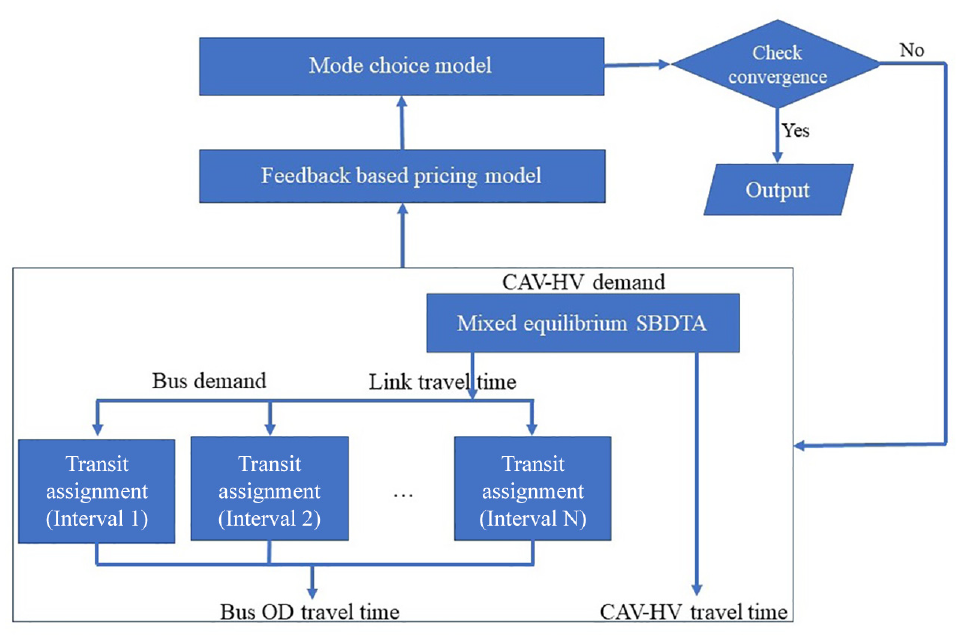
Tri-level methodological framework.
Generalized Cost Functions
Three available modes—buses, UE-seeking HVs, and SO-seeking CAVs—are denoted by 1, 2, and 3, respectively (M = {1,2,3}). A generalized cost function consisting of the monetary cost and travel time weighted by the value of travel time (VOTT) is defined to determine the travel disutility associated with each mode. Although it may be easy to show the benefits of transport improvements that bring higher speeds and level of service, the estimation of their dollar value saving is significantly complicated. Numerous studies have been conducted to determine the VOTT; however, it is still a controversial topic for researchers and practitioners. One stream is based on the marginal productivity of working time and the other stream is based on consumer behavior. The first stream is mainly theoretical whereas the latter requires stated preference surveys and empirical analysis to independently estimate the VOTT. Legaspi and Douglas ( 24 ) conducted a comprehensive study and estimated the VOTT considering travel mode, income level, and trip purpose in NSW, Australia. Following this study, we assume $15.14 per hour and $14.39 per hour as the VOTT of HVs and bus users, respectively. For CAVs, VOTT is expected to fall by 20% to 50% ( 25 – 29 ). However, several studies in the literature also suggest the stability or even an increase in VOTT estimation for CAVs ( 30 – 33 ). They mainly argue that CAVs will operate similarly to conventional cars for vehicle states (idling, cruising, accelerating, and decelerating), and people are less likely to spend their time doing in-vehicle multitasking. Given there is still no consensus on the VOTT of CAVs, here we assume the same VOTT as the HVs in this study. This assumption does not affect the validity and applicability of the proposed modeling framework. Note that the mode choice decision between AV and HV can be influenced by various factors including the energy consumption, availability of the alternative, and personal preferences that are beyond the scope of the current study and can certainly be explored in future studies.
The assumed generalized cost functions for the three alternative modes are as follows:
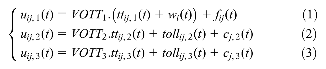
where the time-dependent travel time from origin
In this study, we utilize a congestion pricing scheme that differentiates between HVs and CAVs concerning their route choice behavior. SO-seeking CAVs whose routing is controlled by a central agency may have to take longer routes to avoid congested links and reduce total system travel time. In return, they will receive a discount on the congestion toll. To do so, a general optimal toll is determined using a feedback-based control strategy for every toll interval, which will be discussed later. The SO-seeking CAVs are subject to a lower congestion charge for entering the pricing zone compared with the UE-seeking HVs. No toll is imposed on buses. We explore three different discount levels for CAVs to investigate the performance of the two-rate pricing strategy on the traffic patterns, average toll rate, and total revenue.
Mode Choice Model
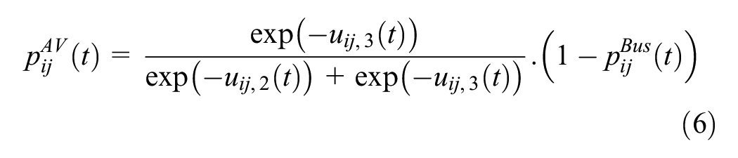
Having determined the origin–destination (OD) generalized travel costs of available alternatives, the probability of choosing each mode is estimated using a discrete choice modeling approach. In this study, we use a simple two-level nested logit model in which the upper level has two alternatives of bus and private car and the lower level has two options of CAVs and HVs. The mode choice model estimates the probability of each person’s trip using a bus, CAV, and HV. The probability of selecting any alternative decreases with a decrease in the utility of the alternative. The nested logit model can be mathematically expressed as:
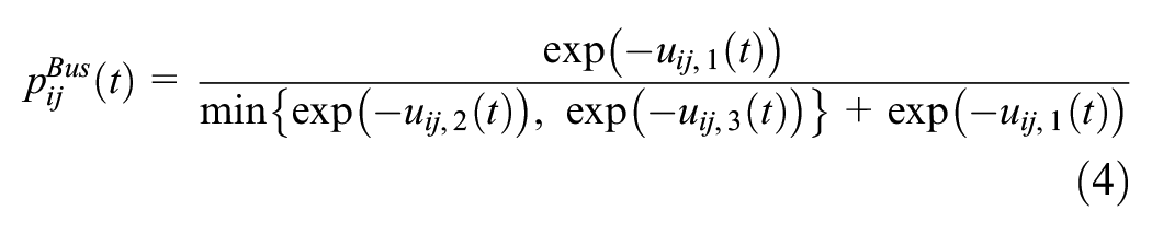
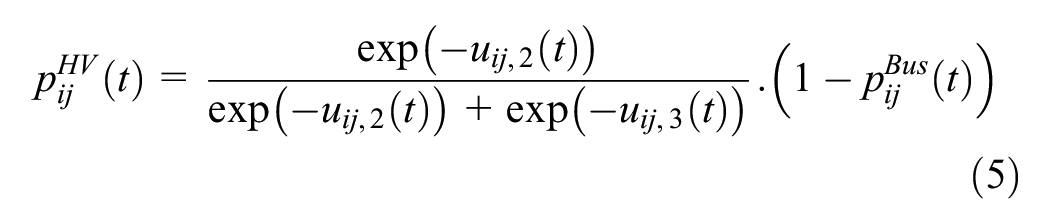
Therefore, the number of trips made by each travel mode between origin
Feedback-Based Congestion Pricing Controller
Feedback-based control is a widely used approach in traffic engineering to control inflow to the network or part of the network to achieve a predetermined setpoint. Integration of feedback-based controller and NFDs for congestion pricing and perimeter control applications is already well studied ( 17 , 18 , 34–37). Generally, the traffic inflow is regulated such that the NFD does not enter the congested regime and operates at its maximum throughput.
As previously mentioned, traffic flow is multimodal and the interaction between different travel modes sharing the limited road space needs to be taken into account. To evaluate traffic dynamics in bimodal networks, the 3D-NFD (or 3D-pNFD) is an effective tool to model the traffic state evolution in a dynamic environment.
In 3D-NFD, the network travel production is expressed as a function of accumulation of private and public transport vehicles. Car production


Similarly, production

Following Zheng et al. ( 18 ) and Gu et al. ( 34 ), we use the estimated 3D-pNFD within a discrete proportional-integral (PI) controller framework with the following general form:
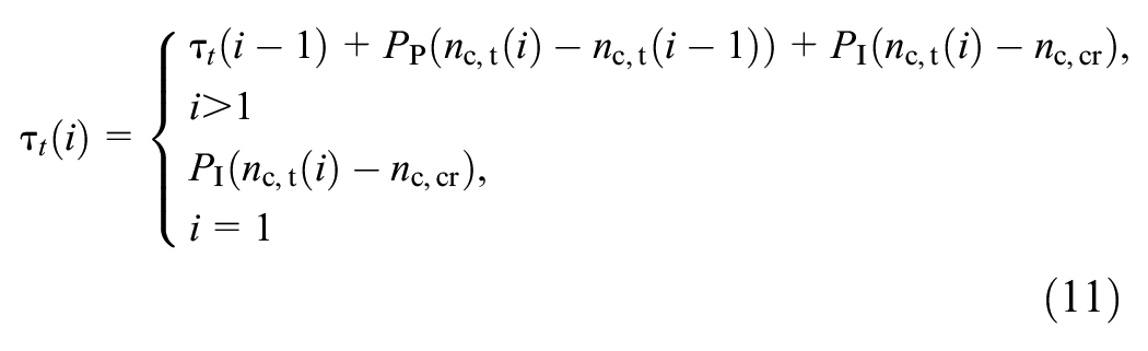
where

where
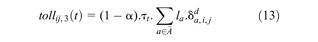
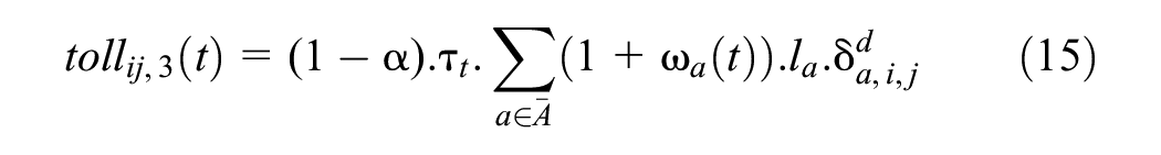
Although the numerical experiments presented later in the paper follows the formulated distance-based toll, the toll function can be extended to include link-level congestion as in Mansourianfar et al. ( 10 ). We argue, however, that distance-based pricing is practically seen already, and that link-specific congestion-based pricing, although theoretically computable, could be hard to implement in practice (constant monitoring of each link for each vehicle). Still, the distance-based toll can be expressed as follows:
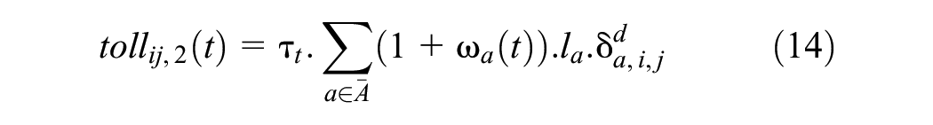
where
Integrated Mixed Equilibrium SBDTA and Transit Assignment Model
Unlike static traffic assignment models, dynamic models update the shortest path set during each assignment interval; that is, they differentiate between travelers departing at different time intervals. Therefore, dynamic models are very useful for assessing intelligent transportation system applications such as dynamic congestion pricing, mode choice modeling, and so forth. Dynamic traffic assignment models can be broadly categorized into two classes, simulation-based and analytical approaches (see Peeta and Ziliaskopoulos [ 38 ] for a comprehensive overview). The simulation-based approach, which was originally proposed by Mahmassani and Peeta ( 39 ) and Mahmassani ( 40 ), avoids the need for link cost and link exit functions and makes the DTA problem more tractable, particularly in large-scale networks. Mahmassani and Peeta ( 39 ) applied an iterative dynamic solution algorithm to study 100% UE- and 100% SO-seeking traffic network patterns. Mansourianfar et al. ( 10 ) extended their model to be applicable to mixed autonomy traffic networks where two classes of vehicles with different microscopic and routing behaviors (UE-seeking HVs and SO-seeking CAVs) are present. The proposed mixed equilibrium SBDTA conforms to the three-step traditional setup, including standard network loading, path set update, and path assignment adjustment, which are applied sequentially and iteratively to all the Time-Dependent Origin Destination matrices. The extension also allows for varying reaction times and link capacities depending on the proportion of CAVs on a link. It also includes a hybrid termination criterion to ensure the convergence of the mixed equilibrium SBDTA algorithm. For more details, refer to Mansourianfar et al. ( 10 ).
Transit assignment models are relatively more sophisticated than traffic assignment models. In addition to the common features of the traffic assignment problem, the transit assignment problem includes other unique challenging issues such as transfers, in-vehicle travel time, boarding and distance fare, waiting time at stops, crowdedness inside vehicles, and so forth. Traffic and transit assignment models can be integrated and applied in multimodal networks to assess policies that affect the performance of both road and transit networks. However, integrating traffic and transit assignment models and allowing modal shift between transportation modes are less explored research topics. In the literature, very few studies have investigated the effect of road congestion on transit assignment. For example, Oliveros and Nagel ( 41 ) calibrated a schedule-based transit assignment model in which the effect of road congestion on bus journey time was overlooked. Kamel et al. ( 42 ) built a simulation-based traffic and transit assignment model for the network of the Greater Toronto Area. The proposed assignment model is mesoscopic, dynamic, and UE-seeking, which includes surface transit routes and takes into consideration the in-vehicle crowdedness and congestion effects on bus travel times.
In this study, we extend the mixed equilibrium SBDTA model developed in our previous study ( 10 ) and integrate it with a transit assignment model to generate the aggregate travel flows in a bimodal network. One of the outputs of the mixed equilibrium SBDTA is time-dependent link travel time that is fed into the transit assignment model to account for the actual road congestion effects on the generalized cost of bus travel. For a detailed discussion on the solution algorithm and convergence properties, refer to Mansourianfar et al. ( 10 ).
Numerical Experiments
Estimation of 3D-NFD
This section aims to investigate the performance and applicability of the proposed framework in a large-scale traffic network. Figure 2 depicts the configuration of the extracted subnetwork from the Greater Melbourne area network model. The gray lines represent private car links and the black lines and the black empty circles represent the bus routes and the bus stops, respectively. The red rectangle depicts the congested CBD of Melbourne where we apply the proposed congestion pricing scheme. The extracted subnetwork consists of 4,450 links, 2,163 nodes, and 416 centroids. The transit network consists of 70 bus lines, 1,014 bus stops, and their corresponding timetable that were imported using the available General Transit Feed Specification (GTFS) framework ( 43 ).
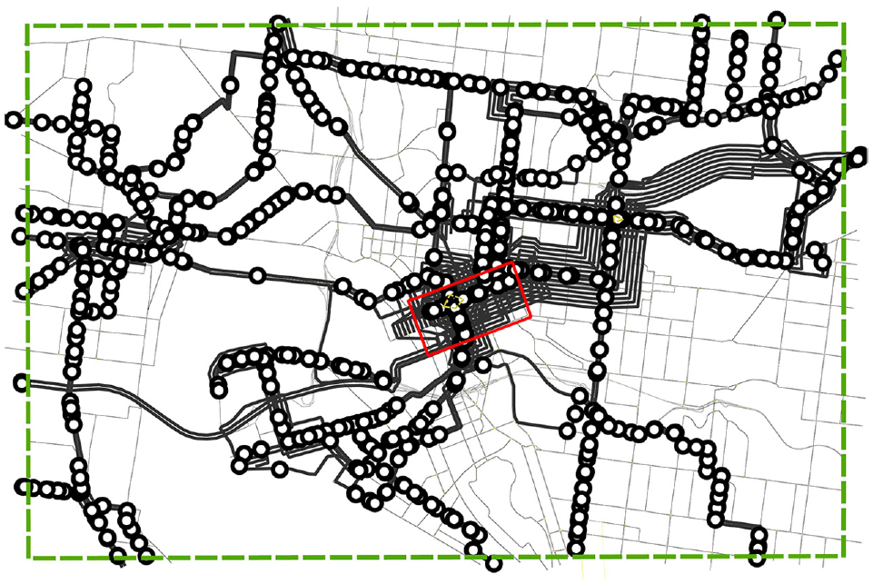
The extracted subnetwork from the Greater Melbourne area model. The red rectangle depicts the central business district (CBD) of Melbourne, which is designated as the congestion pricing area.
In this analysis, we aggregate data into 15-min intervals and use the speed information of private vehicles (i.e., CAVs, HVs) and public transport vehicles in the CBD. We observe that the private car speed drops to 14 km/h from 8 to 9 a.m. but recovers and reaches 25 km/h at the end of the simulation period at 10 a.m. The average speed of public transport vehicles is around 12 km/h, showing a slight decrease to 10 km/h during peak hour (see Figure 3a). Figure 3b shows the number of travelers in private vehicles and buses, stacked by mode. We observe that the passenger accumulation is mostly made up of private car passengers. However, during the peak period (8 to 10 a.m.) the number of bus passengers increases significantly from 9:30 to 10:00 a.m. This suggests the necessity of providing bus priority schemes, specifically in the pricing area, that can have considerable impact on overall passenger mobility.
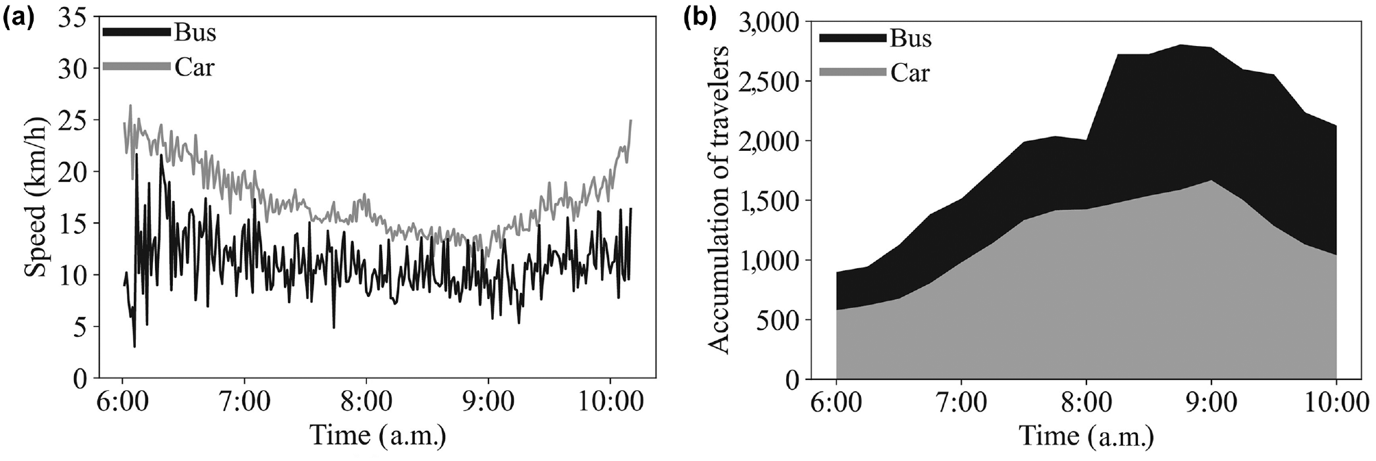
Time profiles of (a) speed and (b) passenger accumulation by mode in the central business district (CBD).
Figure 4 shows the resulting 2D-NFD of both travel modes for the CBD. As expected, both the accumulation and production range of private vehicles are considerably more than for the bus mode. The maximum car travel production is achieved at the accumulation of 1,200 vehicles (Figure 4a). Although the car travel production decreases once the critical accumulation is reached, the bus 2D-NFD mostly remains in the free flow regime with maximum trip production of 300 vehicle kilometers per hour associated with 25 buses as the public transportation accumulation in the CBD (see Figure 4b). Figure 4, c and d , shows the fundamental relationship between average speed and accumulation in the CBD. Unlike Figure 4c, Figure 4d shows the bus speed that is highly scattered, ranging from 5 to 20 km/h. It is mainly attributed to the short time interval for calculating bus speed (1 min) that increases the bus speed variation over the whole simulation period. The maximum observed travel speed of private cars is 35 km/h, whereas it drops to below 10 km/h at the accumulation of 1,400 vehicles.
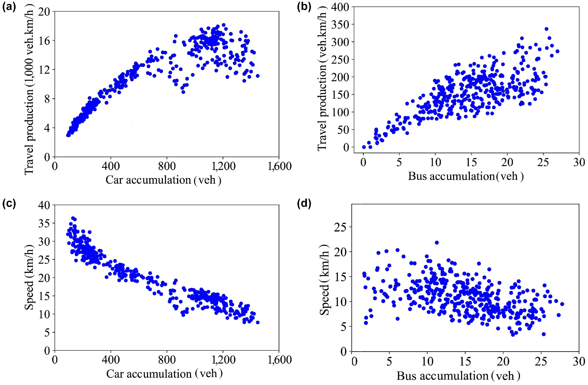
Simulated two-dimensional network fundamental diagrams (2D-NFDs) of the central business district (CBD) by mode.
To obtain a general understanding of the modeled bimodal network, we also estimate the 3D-NFD of the CBD, which exhibits the total travel production (car and bus) as a function of car and bus accumulation. Figure 5 illustrates that the maximum experienced travel production can reach 18,000 vehicle kilometers per hour where the car and bus accumulations are at 1,200 and 22 vehicles, respectively. Because of the fixed timetables of the bus routes, the 3D-NFD only includes limited data points for the public transport accumulation. In the following section, linear models are estimated based on the simulation data to reproduce a more informative 3D-NFD and 3D-pNFD. The estimated 3D-pNFD is used to determine the target average car accumulation or density in the CBD as the set point in the PI controller in the congestion pricing scheme.
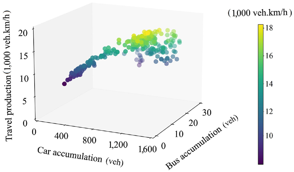
Simulated three-dimensional-passenger network fundamental diagram (3D-pNFD) of the central business district (CBD).
A Statistical Model for the 3D-NFD and 3D-pNFD Estimation
Using the simulation results, we fit a statistical model to quantify the macroscopic traffic flow relationships and estimate a more functional and informative 3D-NFD. In the case that no traffic data are available, the estimated form is still valid (
44
). Geroliminis et al. (
22
) proposed an exponential function to link car and bus accumulations with the total flow. However, Loder et al. (
23
) introduced two simple linear equations to estimate the speed of the car and bus given the vehicle density in a bimodal network. To account for different region size, vehicle density was used rather than vehicle accumulation. In this study, we deal with a single-region problem. Therefore, we determine the network travel production as a function of car and public transport vehicle accumulations rather than density (see Equation 16). To obtain the 3D-NFD using Equation 16, we estimate the speed of cars and buses

Following Loder et al. (
23
), we use Equations 17 and 18 to link car and bus speeds to the accumulation of cars and buses.


Table 1 shows the estimated parameters of the 3D-NFD for Melbourne CBD network, based on the simulation results (06:00 to 10:00 a.m. at 1-min intervals with a total of 240 data points) described in the numerical experiments section on estimation of 3D-NFD. Using the ordinary least squares technique, model estimates are determined. Comparing the marginal effects of car and bus accumulations, a slightly higher decrease in car speed would occur by one additional unit of bus accumulation rather than one car. Considering public transport speeds, we observe 3 km/h for the constant and around 0.43 km/h increase in public transport speeds by increasing one unit in car speeds.
Estimated Model Parameters for the Three-Dimensional-Network Fundamental Diagram of Melbourne Central Business District Network.
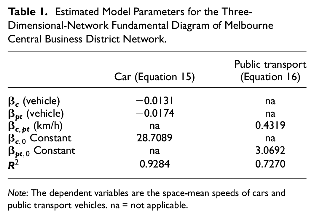
Note: The dependent variables are the space-mean speeds of cars and public transport vehicles. na = not applicable.
Given the estimated 3D-NFD, car and bus speeds
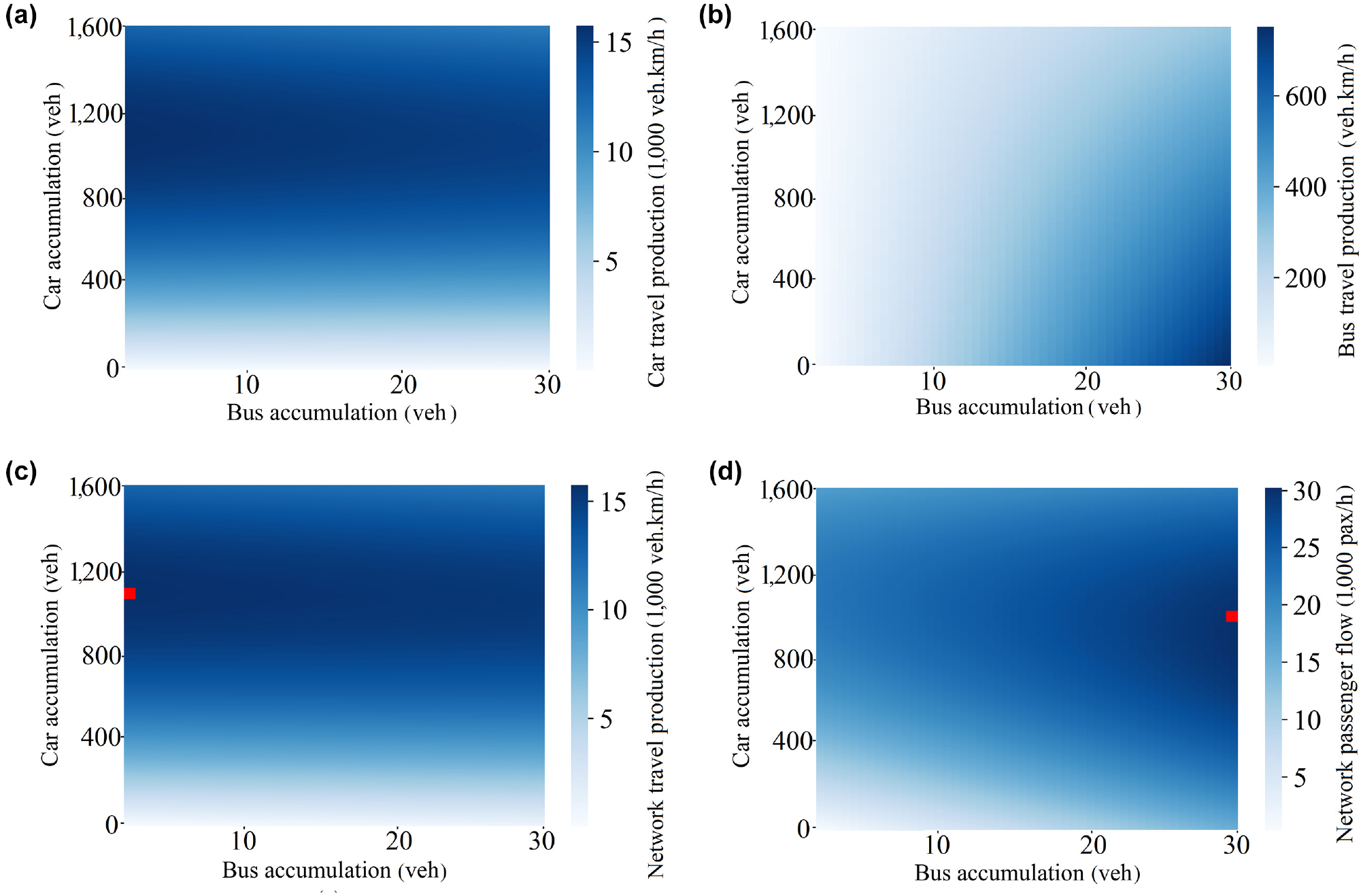
(a) Car travel production vs. accumulations, (b) bus travel production vs. accumulations, (c) network travel production vs. accumulations, and (d) network passenger flow vs. accumulations. The red dot is the identified optimal solution.
To determine the optimal allocation of travelers to each mode, the network travel production, and network passenger production are estimated over the accumulations range of the simulation data. In a bimodal network, public transport vehicles are generally the more efficient modes of travel than cars because of higher passenger occupancy; they allow us to investigate the network passenger flow carried by both buses and cars (
22
,
23
).The total passenger flow

where
The low average bus speed, which is further reduced in the congested CBD by private cars, results in smaller travel production compared with private cars. In the case of incorporating the 3D-NFD in the PI controller, full priority is given to private vehicles to maximize network travel production. According to Figure 6c, the maximum travel production is achieved at the accumulation of only 1,160 private cars in the CBD. However, given the higher occupancy capacity of buses, network passenger flow increases with greater accumulation of public transport vehicles. Although the public transport agency can increase the bus frequency theoretically, in practice this is less likely to happen in the short term because of the operational costs, fixed timetables, and other practical challenges. Therefore, the bus inflow is exogenously determined. If we select an unattainable high bus accumulation, the pricing control will target fewer private cars than the optimum amount corresponding to the actual bus accumulation in the pricing area.
Figure 6d suggests that smaller car accumulation of 1,050 vehicles ensures an accumulation of 30 buses in the CBD. Therefore, we select critical car accumulation as 1,050 as a setpoint in the proposed PI controller to optimize passenger flow in the CBD. Once the 3D-pNFD-based pricing control is applied, we check and verify whether the accumulation of 30 buses is attained given the fixed timetable of bus routes.
Results and Discussion
The proposed framework applies a general toll rate to the pricing zone that is dynamically optimized and imposed on the UE-seeking HVs. A discount rate on the congestion charge is applied for SO-seeking CAVs entering the pricing zone. Discount rate value
Here, we explore three scenarios with different discount rates for SO-seeking CAVs. Given the determined toll rates, the probabilities of choosing different modes are estimated through a mode choice model and fed back into the SBDTA model. This process continues iteratively until an equilibrium point in the system is identified. Table 2 presents the average toll rate during peak period, the total distance traveled by HVs and CAVs, and the total revenue for three different scenarios.
Estimated Average Toll Rate, Distance Traveled, and Total Revenue for Different Simulated Scenarios
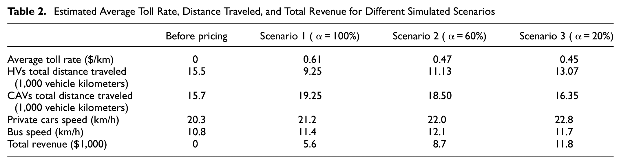
In Scenario 1, SO-seeking CAVs are entirely exempted from paying the toll. In Scenarios 2 and 3, SO-seeking CAVs receive 60% and 20% discounts on the average toll rate, respectively. In Scenario 1, CAVs can freely travel into the pricing zone. Therefore, to keep the pricing area uncongested a considerably high toll is determined and imposed on HVs. The average toll rate is determined as $ 0.61 per kilometer, which is the largest charge among the other scenarios. This high toll rate considerably reduces the distance traveled by HVs in the pricing zone and, as a result, the total revenue in a single day for the pricing period is only $5,600. Although the average toll decreases in Scenario 2, the total revenue increases to $8,700 during the pricing period. The reduced average toll would bring more HVs into the pricing zone. Offering only 20% discount on tolls for CAVs in Scenario 3 further decreases the average toll rate. Therefore, the distance traveled by HVs increases, whereas the distance traveled by CAVs decreases, and the gap between them shrinks while the total revenue increases to $11,800. All pricing scenarios successfully keep the pricing area uncongested, which increases the average speed for both private cars and buses by 5% to 12%.
Having calculated the generalized cost of each travel mode, we next determine the resulting mode share in the pricing zone for each scenario. Table 3 illustrates the modal split between HVs, CAVs, and public transportation in the CBD under different scenarios. Generally, the share of UE-seeking HVs is higher than others because they take the paths with the shortest travel time and benefit from the higher utility. However, it varies depending on the pricing scenarios. In Scenario 1 and during the pricing period, imposing tolls on HVs reduces the corresponding share by almost 10% (from 49% to 39.4%). Accordingly, the mode shares of CAVs and buses increased by 7% and 3%, respectively. Reducing the discount rate on CAVs in Scenarios 2 and 3 leads to a modal shift from CAVs to HVs whereas the bus share remains almost stable.
Mode Shift between Human-Driven Vehicles (HVs) (in Blue), Connected and Automated Vehicles (CAVs) (in Orange), and Buses (in Green) With and Without Pricing in the Central Business District Under Different Scenarios
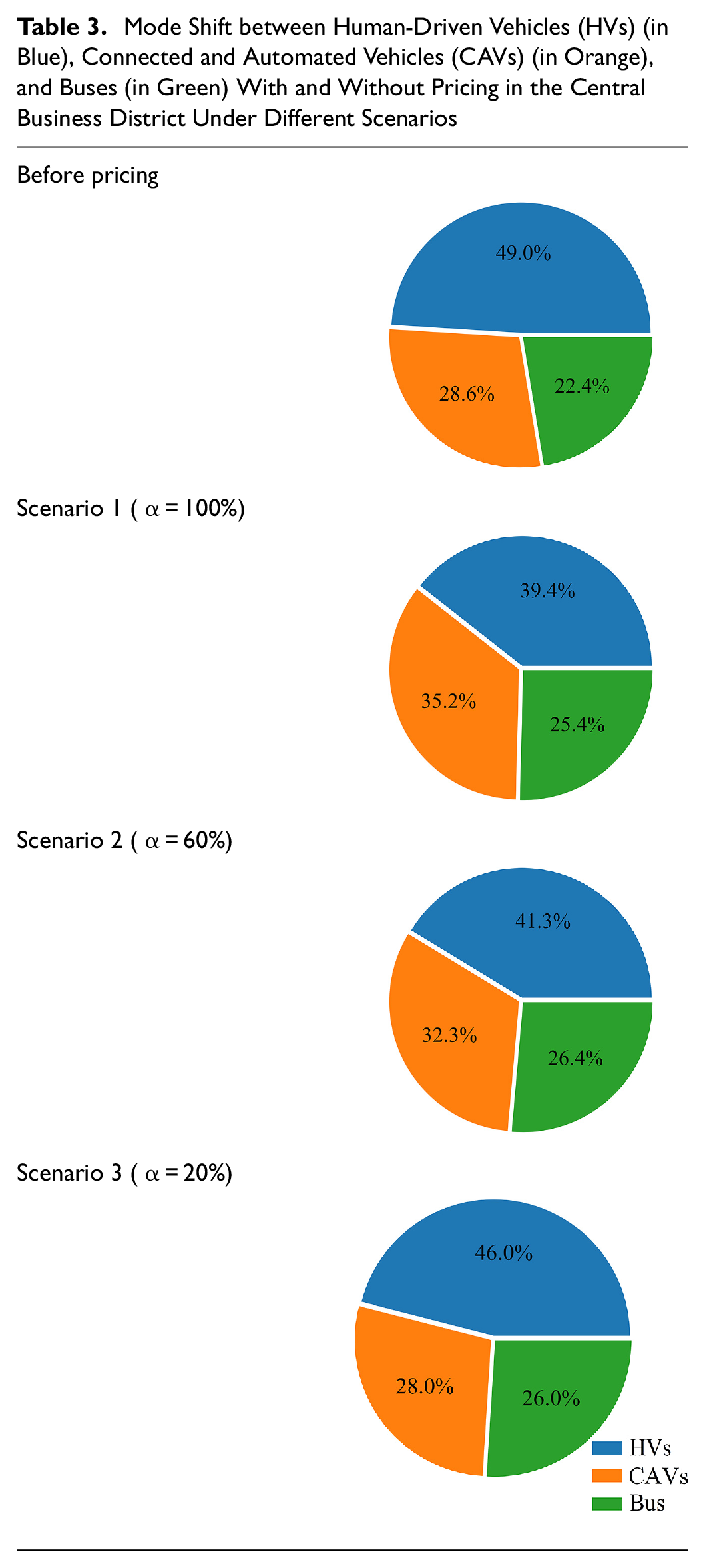
Figure 7 compares the 2D-NFD of the CBD with and without pricing. As expected, implementing congestion pricing improves the overall performance of the bimodal network. Imposing congestion tolls keeps the traffic condition in the free flow state and improves the mobility of buses in the pricing zone. Figure 7a suggests a smaller maximum car accumulation compared with the non-pricing scenario to give more space and priority to public transport vehicles to freely enter and travel in the pricing zone (see the bus accumulation increase in Figure 7b). The average speed of private cars and buses increases under all three pricing scenarios. Figure 7, c and d , suggests that the maximum travel speed of cars and buses can reach 45 and 25 km/h, exhibiting an average 10% improvement.
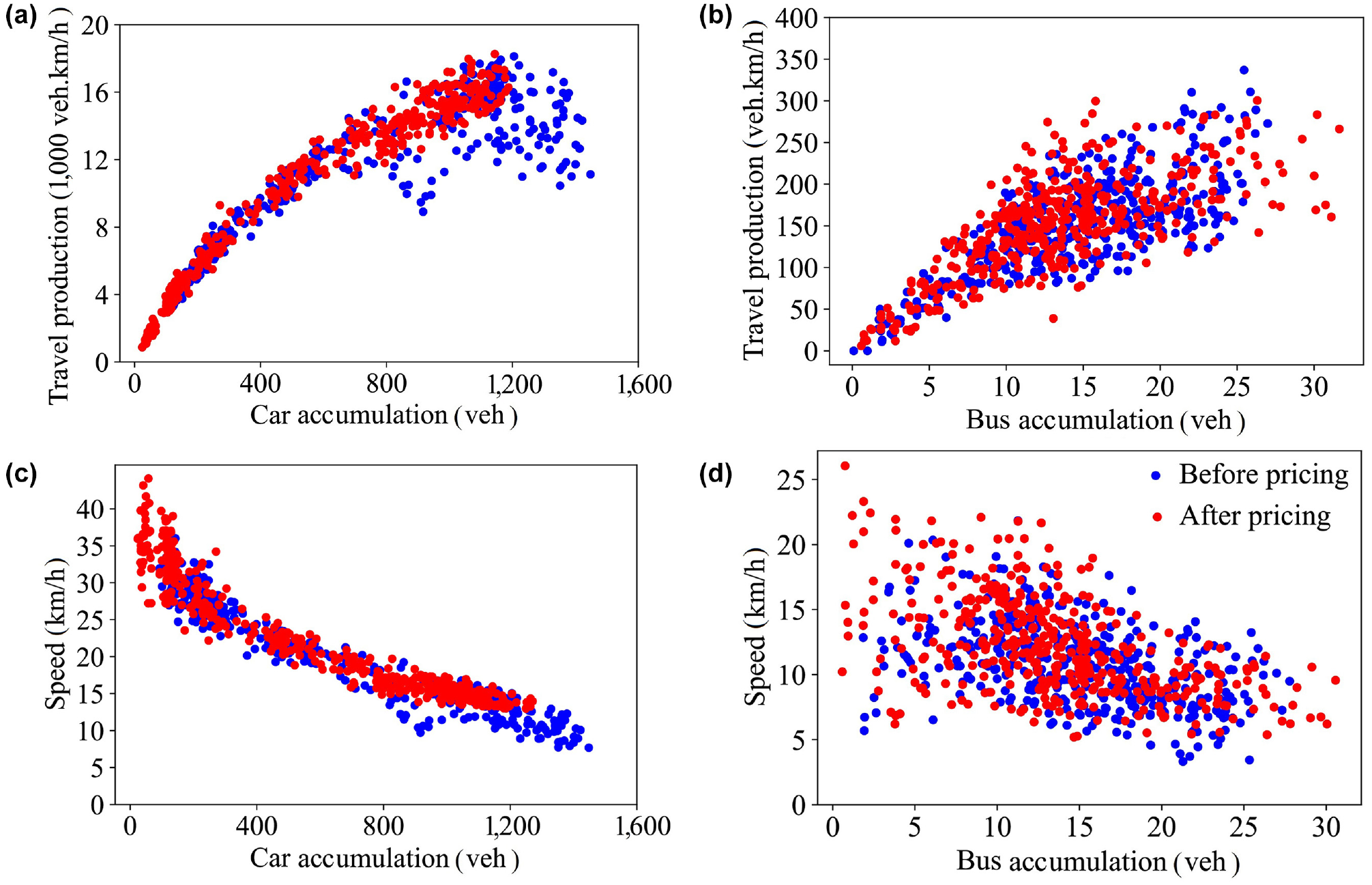
Two-dimensional network fundamental diagrams (2D-NFDs) of the central business district (CBD) by mode when pricing is applied.
Conclusion
Understanding and modeling the interaction between different travel modes sharing the road space in bimodal mixed autonomy urban road networks is a less explored area of research. Few past studies have explored the traffic dynamics of private and public transport vehicles simultaneously at the network level using 3D-NFD ( 23 , 44 ). 3D-NFD (or 3D-pNFD) relates the network travel production (or network passenger production) and the accumulation of cars and buses that can be applied as a practical tool to monitor and optimize the inflows for both private and public vehicles.
The study presents a methodological advancement by integrating multimodality into NFD-based pricing for the transport network, building on the groundwork laid by Mansourianfar et al. ( 10 ). In the present study, we extend the modeling framework to include elastic demand and a multimodal network, incorporating transit assignment that implicitly considers vehicle capacity and service frequency. The implemented model reflects Melbourne’s public transport system, providing details on the bus network with information obtained from GTFS data. Results suggest that the simulated demand for public transport can be accommodated by existing services, attributing the small change in bus mode share to the assumed mode choice model. The primary goal of the numerical experiment presented in this study is to demonstrate the applicability of the proposed pricing model with elastic demand assumptions, rather than estimating a realistic mode choice model, which would require real-world survey data and sophisticated estimation approaches.
In this study, we proposed a 3D-pNFD-based congestion pricing in a mixed autonomy bimodal network that keeps the pricing area uncongested for different competing modes including buses, SO-seeking CAVs, and UE-seeking HVs. We developed an iterative tri-level model for mode choice, pricing, and route choice in which the lower level generates mixed equilibrium traffic flows. The mid-level finds the optimal toll rates using 3D-pNFD-based feedback controller. A nested logit mode choice model is also applied to capture travelers’ preferences toward three available modes. To incentivize CAVs to follow the SO routing, they are provided with a discount on the congestion toll. Three scenarios were explored with different discount rates to investigate the effect of incentive plans on the mode choice behavior of road users and resulting traffic dynamics in the pricing zone.
The estimated 3D-NFD for the designated pricing zone suggests that the maximum travel production is achieved when the car and bus accumulations are 1,160 and zero, respectively (see Figure 6c). As a result of the low average bus speed in the congested CBD, they generate smaller travel production compared with private cars. So, in the case of incorporating the 3D-NFD in the PI controller, priority is given to private vehicles to maximize network travel production. However, public transport vehicles are a more efficient mode of travel than cars because of the higher passenger occupancy. To maximize network passenger production in the CBD instead of travel production, we estimate a 3D-pNFD that suggests a smaller car accumulation value to guarantee a larger bus inflow to the CBD. Given fixed public transportation timetables, if we select an unattainable high bus accumulation, the pricing control will target fewer private cars than the optimum amount corresponding to the actual bus accumulation in the pricing zone. According to Figure 6d, the smaller car accumulation of 1,050 vehicles ensures an accumulation of 30 buses in the CBD. Therefore, we select critical car accumulation as 1,050 as a setpoint in the proposed PI controller to optimize passenger flow in the CBD and improve bus mobility in the pricing zone.
Given the determined bus accumulation, the proposed 3D-pNFD pricing scheme aims to target the corresponding optimal car accumulation in the pricing zone. Generally, the share of UE-seeking HVs is higher than other modes. The results from Scenario 1 (SO-seeking CAVs receive 100% discount) show that imposing tolls on HVs (i.e., $ 0.61 per kilometer on average) reduces the corresponding mode share by almost 10% in the pricing zone (from 49% to 39.4%). Instead, the mode shares of CAVs and buses increased by 7% and 3%, reaching 35.2% and 25.4%, respectively. In Scenarios 2 and 3, CAVs receive discounts of 60% and 20% on the average toll rate, respectively. Reducing the discount rate on CAVs leads to a modal shift from CAVs to HVs whereas the bus share remains almost stable (almost 26%). Although the average toll decreases in Scenario 2 (i.e., $ 0.47 per kilometer on average), the total revenue increases during the pricing period. The reduced average toll would bring more HVs into the pricing zone and increase the total revenue. Offering only 20% discount on tolls for CAVs in Scenario 3 further decreases the average toll rate ($ 0.45 per kilometer on average). Therefore, the distance traveled by HVs increases, whereas the distance traveled by CAVs decreases. In addition, all pricing scenarios consistently keep the pricing area uncongested, which results in an increase in average speeds of private car and buses. In this study, we assumed that the VOTT of CAVs is the same as that of HVs. As future research directions, the effect of different VOTT for CAVs on the pricing outcomes could be explored. Integrating different incentive programs for public transport within the congestion pricing framework could also be further explored.
Although the study used a real-world network model of Melbourne, the assumed mode choice model only partially captures travelers’ preferences. The simplicity of the model, which considers parking costs but not trip costs for CAVs and HVs, may limit the realism of behavioral parameters (45, 46). We acknowledge that a more realistic mode choice model, incorporating comprehensive trip cost considerations would provide more accurate insights into travelers’ preferences. However, because the study’s primary focus is on proposing a multimodal NFD-based pricing methodology, the lack of a detailed mode choice model is recognized as a limitation. Comprehensive survey data and sophisticated choice modeling, necessary for a more realistic representation, were beyond the scope of this study. Consequently, the presented numerical experiments, although valuable for demonstrating the applicability of the theoretical modeling framework, may not have policy implications because of the inherent limitations in the mode choice model.
Footnotes
Author Contributions
The authors confirm contribution to the paper as follows: study conception and design: M.M., Z.G. and M.S.; data collection: M.M.; analysis and interpretation of results: M.M., Z.G. and M.S.; draft manuscript preparation: M.M., Z.G. and M.S. All authors reviewed the results and approved the final version of the manuscript.
Declaration of Conflicting Interests
The author(s) declared no potential conflicts of interest with respect to the research, authorship, and/or publication of this article.
Funding
The author(s) received no financial support for the research, authorship, and/or publication of this article.