Sage Journals: Discover world-class research

Abstract

Machine-learning methods can assist with the medical decision-making processes at the both the clinical and diagnostic levels. In this article, we first review historical milestones and specific applications of computer-based medical decision support tools in both veterinary and human medicine. Next, we take a mechanistic look at 3 archetypal learning algorithms—naive Bayes, decision trees, and neural network—commonly used to power these medical decision support tools. Last, we focus our discussion on the data sets used to train these algorithms and examine methods for validation, data representation, transformation, and feature selection. From this review, the reader should gain some appreciation for how these decision support tools have and can be used in medicine along with insight on their inner workings.

Keywords

medical decision support machine learning learning algorithms review

Emergence of Computer Decision Support in Medicine

Medical decision making requires clinicians of all types to act on patient information with less than all-possible knowledge regarding the patients’ health status. To help manage this uncertainty, computer tools have been developed to assist both veterinary and human health care providers in this decision-making process.^22,58,61,98 Some of these tools have been created to improve information retrieval, some to analyze patients’ records, and others as intelligent tools (using machine learning) to provide direct decision support. Efforts to develop these computational tools go back to the 1950s.^58,62 These early efforts were also documented in a 1979 review assessing strengths and limitations of these early clinical algorithms, databanks, and mathematical models used to support computer-based clinical decision support systems.⁹⁵

Veterinary Medicine

In veterinary medicine, there have been a limited number of studies highlighting the challenges and applications of computers and medical informatics to solve problems in veterinary medcine.^5,6,84 One study evaluated the use of artificial neural networks and case-based, rule-based, and fuzzy logic systems to diagnosis a variety of fish diseases.¹¹⁷ The authors determined that these expert systems proved useful for this purpose. Another study developed a decision support system to help veterinarians with the interpretation of findings from physical examinations.³² A 2013 study reported the ability of machine-learning algorithms to extract syndromic information from laboratory test results received by a veterinary diagnostic laboratory.²⁸ In this study, naive Bayes, decision tree, and rule-based methodologies were shown to achieve relatively good performance. Another study used machine learning to show its potential to diagnose canine visceral leishmaniasis.³¹ In 2016 and 2018, there were 2 studies by Awaysheh et al^10,12 examining the use of machine-learning methods to assist clinicians and pathologists in distinguishing between and identifying key microscopic features of intestinal lymphoma and inflammatory bowel disease in cats. Compared to human medicine, the use of machine-learning methods in veterinary medicine has been very limited.^73,74,104

Human Medicine

In the 1970s, researchers at the University of Pittsburg developed INTERNIST as one of the first human medicine clinical decision support systems.⁷⁶ It was a rule-based expert system designed to diagnose complex internal medicine disorders. These early efforts at codifying the rules used in these systems encouraged the development of more formal methods for representing expert knowledge.¹⁰⁸ Also in the 1970s, MYCIN was developed as another rule-based expert system designed to diagnose and suggest treatments for blood infections. MYCIN’s knowledge base was modeled as a set of if-then rules and certainty factors associated with each diagnosis.⁹⁵

In the 1980s, the INTERNIST knowledge base was used to create other systems, including CADUCEUS and Quick Medical Reference.^67,69 Around this same time, RECONSIDER was developed as a program for generating differential diagnoses given a list of patient attribute values.¹⁵ RECONSIDER’s knowledge base was composed of a corpus of 3262 disease definitions in the form of structured natural language text. DXplain was another system developed in the late 1980s for the purpose of supporting the decision-making process and to diagnose common disorders, such as anemia or heart failure. The system accepted a list of clinical findings and then proposed a diagnostic hypothesis.¹³

Encouraged by results from these early systems, medical researchers developed decision support tools focused on specialty areas of medicine in the 1990s. One such study systematically assessed the use of different computer classification systems for the interpretation of electrocardiograms.¹⁰⁹ In this study, the computer-based diagnoses were compared with those of cardiologists for concordance and did almost as well as the cardiologist in identifying 7 major cardiac disorders. For breast cancer, machine learning, specifically artificial neural network algorithms, were shown to distinguish between benign and malignant lesions more accurately than radiologists.^{1,25,34,36,78} Authors of another breast cancer study showed that the artificial neural network algorithms could be constructed using a very limited number of features (variables used in making predictions such as the number of lymphocytes in a blood sample) and still achieve high accuracy.⁹² The same study demonstrated a way of extracting correlations from the generated neural network to be used in classification of the lesion. Another study also reviewed the literature for different tools and their application in screening for breast cancer;⁴⁵ those authors found that most of the screening technologies used theoretical frameworks. In another study of breast cancer decision support systems, authors reviewed performance of different prediction models following reduction of considered features with intent of reducing model complexity.⁶⁶ With this approach, the authors found classification accuracy only slightly decreased following the reduction of 30 features into 1 dimension while the sensitivity rates increased. In their study, authors used neural network and support vector machine algorithms. A study conducted in 2007 reviewed the application of machine learning and computational systems for diagnosing and predicting biological behavior of prostate, bladder, and kidney cancers.² The authors concluded that machine learning had the flexibility and capability to assist physicians in making clinical decisions. Moreover, the authors argued that machine-learning applications could be superior to standard statistical methods and allowed for more flexibility in the decision-making process. They also suggested that understanding machine-learning methods and their potential would advance the diagnosis and management of cancer care.

For diseases other than cancer, a study in the 1990s assessed the use of machine-learning algorithms to diagnose various sports injuries.¹¹⁸ The study showed a classification accuracy of up to 70% with the naive Bayes algorithm using fuzzy discretization of numerical attributes (converting continuous values into a set of discreet ranges or bins of a single value). In another study conducted in 1998, the same authors developed a system to give recommendations on anti-infective therapy. A prospective study of the scheme showed that its usage led to significant reductions in orders for drugs, excess drug usage, antibiotic-susceptibility mismatches, and costs.³⁰

A 2005 review examined the effects of computer-based clinical decision support systems on clinician performance (97 studies) and patient outcome (52 studies).³⁷ The review included applications used as diagnostic tools, reminders, disease management, and treatment guideline systems. The analysis showed that decision support systems improved the practitioners’ performance in 64% of the studies and improved the patients’ outcome in 13% of the studies. Medical conditions considered in the studies included mental, cardiac, and abdominal disorders.^{20,59,77,89,91,107}

Using decision tree, naive Bayes, and neural network algorithms, a 2008 study developed an intelligent system to predict the likelihood of heart diseases.⁷¹ The study showed that the most efficient model for predicting heart disease was the naive Bayes, followed by ones using neural network and decision tree algorithms. The authors showed that these models were able to answer complex queries and provided detailed guidance to their uses.

In 2012, one study tested the use of decision support systems to diagnose jaundice in newborns.³³ The study used machine-learning algorithms such as Decision tree, neural network, naive Bayes, and others. The findings of the study suggested use of these computer tools could improve the diagnosis of neonatal jaundice. Another 2012 study examined the use of a clinical decision support system for cervical cancer screening by learning from a corpus of 49 293 Papanicolaou cervical cytopathology reports.¹⁰³ The systems accessed patient records and generated patient-specific recommendations based on established but complex clinical guidelines. In this study, the decision support tool identified 2 patients for gynecology referral that were missed by the clinician based on guideline recommendations. Authors highlighted the ability of the tool to learn from free text and suggested that greater use of standardized medical reporting would further increase their benefit in medicine. Many other applications have focused on learning from free text for the purpose of supporting medical diagnostic decision making.⁹⁰

Studies conducted in 2014 developed a decision support system to distinguish between acute respiratory distress syndrome and cardiogenic pulmonary edema.⁸⁸ The system used routine clinical data to arrive at clinical prediction score that had an 81% accuracy. Decision support systems have also been adapted for the use of sound as input. In one such study, researchers developed a system to classify heart sounds taken by stethoscope from patients with normal, pulmonary, and mitral valve stenoses.¹⁰⁰ This system used an artificial neural network algorithm and a feature selection methodology to minimize data complexity and reached a 97% classification accuracy. In another 2014 study, a decision support system was developed to diagnose mild cognitive impairment, with a focus on detection of Alzheimer disease using magnetic resonance imaging (MRI) data.¹¹⁹ Using 10-fold cross-validation with a C4.5 decision tree algorithm, the tool achieved performance (80.2% sensitivity) higher than with support vector machine, Bayesian, and neural network designs. Therefore, the authors concluded that decision tree–type algorithms were best for screening patients for these particular disorders. A more recent study (2016) tested the application of machine learning to predict coronary artery disease using data from noninvasive techniques.¹⁰² Authors tested supervised machine-learning algorithms and showed that the multilayer perceptron neural network algorithm achieved the best performance with 88.4% prediction accuracy compared to multinomial logistic regression, fuzzy unordered rule induction, and C4.5 decision tree algorithms.

Other recent human medicine studies have used computer tools with diagnostic images to guide health care provider decisions. Some examples of these applications include a neural network algorithm to grade gastric biopsy atrophy according to the Sydney system, a neural network algorithm to classify colonoscopy images in patients infected with papillomavirus, a support vector machine algorithm to classify breast tumor ultrasound images as benign or malignant, an unsupervised learning algorithm to diagnose basal cell carcinomas from tissue biopsy images, and an improved neural network algorithm to classify breast tumor mammography images as benign or malignant.^{4,8,25,78,96,114} In the literature, there are many other examples of decision support systems being used to diagnosis specific types of neoplasms involving thyroid, gastric, cervical, pancreatic, brain, and lymphoid tissues.^{3,41,43,48,79,86,94,99}

Classification Algorithms

The output for most decision support tools is a classification prediction (eg, benign or malignant) for the instance (case) being examined based on its attributes or features. The engine driving this output is commonly some form of a machine-learning algorithm. Computer scientists classify machine learning into 3 general categories: supervised, unsupervised, and reinforcement learning.^14,52,54

In supervised machine learning, the algorithm takes a set of instances as an input (called training instances), in which every instance belongs to a particularly known class (label) and has a set of associated features with values. The model then outputs or predicts the classes of the new instances given their features’ values; the results are associated with a particular sensitivity (called accuracy in information science). As an example of a supervised learning algorithm for predicting low- and high-grade mast cell tumors from a cytologic sample, 50 low-grade and 50 high-grade cutaneous mast cell tumors are first classified by histopathology. In this example, there are 100 training instances with 50 cases labeled in each of the 2 classes (low and high grade). Each of these 100 cases also had a prior fine-needle aspirate cytologic examination. A defined list of cytologic features was captured from each of the cases (eg, anisocytosis scale 1–5, multinucleation yes/no, number of granules scale 1–5, etc). These captured cytologic features are combined with the histologic class label (high or low grade) for the particular case to make the set of 100 training instances. The instances are then used to train the supervised algorithm for it to learn which cytologic features are associated with the low- and high-grade tumors. Based on the learning pattern from these instances, the supervised algorithm can then predict the low- and high-grade classification of new cases based on observed cytologic features.

In contrast, unsupervised methods learn from instances without knowledge of their predefined classes; clustering algorithms are one such example. Reasons for using a tool of this type might be that the classes for the instances are unknown, historic data for training the algorithm are unavailable, or the user may wish to explore novel classifications for the data. Continuing with the earlier mast cell tumor example, in the unsupervised method, the cytologic features from 100 mast cell tumors are collected. These 100 instances are then analyzed by the algorithm, which attempts to gate the cases into distinct cohorts by optimizing differences found within the cytologic features. In this approach, the classifier may identify 3 or 4 subpopulations of cases. While these cases are not assigned a traditional class label such as low or high grade, each of these identified classes may have some clinical relevance, warranting further investigation.

In the third type of learning, reinforcement, the learning algorithm is not informed as to what actions must be taken but instead tests the reward of different actions to arrive at the most rewarding choice (eg, convolutional neural networks for image analysis and Monte Carlo methods).¹¹² A reinforcement algorithm has similarity to the supervised approach in that class labels are assigned to each instance and the algorithm is trained as before. However, with this method, the pathway to the correct classification is optimized by feedback from less tangible factors such as cost, time, distance, and so on. As an example, there are many routes to drive from one city to another, but some routes are better. Reinforcement algorithms tend to be used in association with various types of neural networks and work well when dealing with complex real-world problems.

With this basis for understanding, we will now examine in more detail 3 supervised learning algorithm architypes: (1) naive Bayes, (2) C4.5 decision tree, and (3) artificial neural network. While these 3 are only a small fraction of the available algorithms used in decision support tools, they are very common, are well studied, and serve as models from which many others are derived. A mechanistic understanding of these 3 will give the user insight on the workings, strengths, and limitations for these and many others.

Naive Bayes

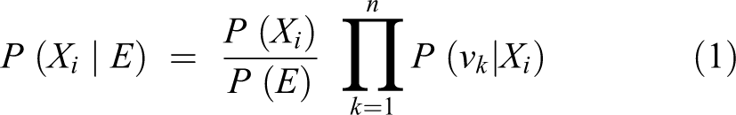
The naive Bayes classifier is simple and efficient. It is derived from the Bayes theorem, which can be used to predict the class of new events using probabilities learned from training with historic data. But, unlike traditional or nonnaive Bayesian classifiers, naive Bayes uses a computationally easier learning process while still maintaining good classification performance. In traditional Bayesian algorithms, computational complexity lies in calculating dependencies and their probabilities as shown by connecting arcs between training attributes and classes as well as between the training attributes themselves. Furthermore, the dependency relationships used in traditional Bayesian systems are commonly created with the help of a domain expert who understands the pathogenesis of the classes being predicted (Fig. 1). However, the naive Bayes model assumes independencies between all the input attributes (no interconnections) with only direct relationships to the outcome classes in the model (Fig. 2).²⁷ Based on the Bayes theorem, the selected class (or predicted one) will be the one that maximizes P (X_i |E) = P (X_i ) P (E | X_i ) / P (E), where X_i represents the ith class, E represents the test example, P (A | B) denotes the conditional probability of A given B, and the prior probabilities are estimated from the training sample. If n represents the number of attributes that are independent given the class, then P (E | X_i ) can be decomposed into the product P (v₁ | X_i )…P (v_n | X_i ), where v_k is the value of the kth attribute in the example E. Therefore, based on naive Bayes, the chosen class should be the one that maximizes

Figure 1.

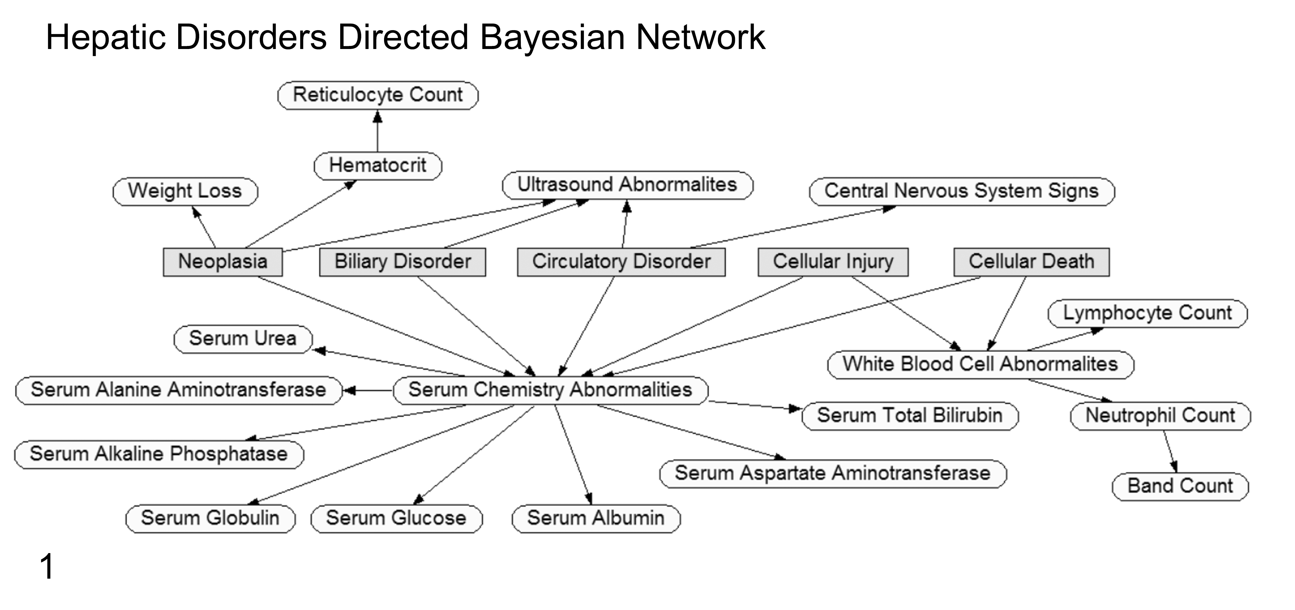
Graphical example of a directed Bayesian network (Netica; Norsys Software, Vancouver, Canada) for predicting 5 hepatic disorders. Classification or disorder nodes are rectangular/gray. Input evidence nodes are oval/unshaded. The connecting lines (arcs) indicate the conditional dependence (causal or correlation relationship) between nodes being used as evidence to predict the probabilities for the outcome disorder nodes. Defining these relationship pathways is the distinguishing feature of a “directed” Bayesian network. For predicting the disorder classification of a new case, observed findings for the evidence nodes are compared to historic probability states for these nodes, and then the Bayes theorem calculates the updated probability state of the disorder nodes.

Figure 2.

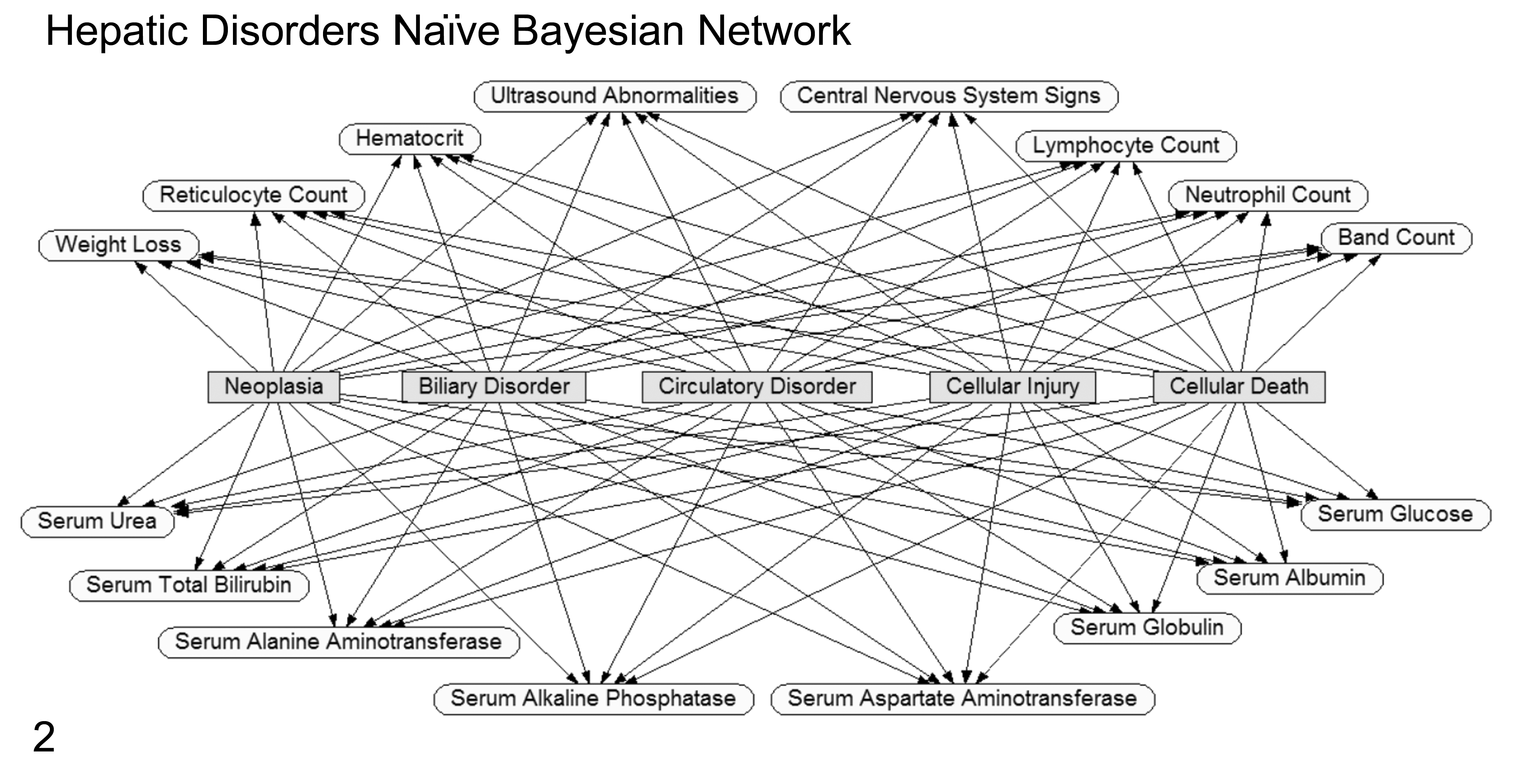
Graphical example of a naive Bayesian Network (Netica; Norsys Software) for predicting the same 5 hepatic disorders as shown in Figure 1. Classification or disorder nodes are rectangular/gray. Input evidence nodes are oval/unshaded. In this example, the evidence nodes are all independent of each other with a connecting line (arc or relationship) only occurring between the evidence node and the disorder nodes. The independence of evidence nodes is the distinguishing feature of a “naive” Bayesian network. For predicting the disorder classification of a new case, findings for the evidence nodes are compared to historic probability states for these nodes, and then the Bayes theorem calculates updated probabilities for all of the prediction disorder nodes. Some of the evidence nodes shown in Figure 1 have been removed for simplicity.

P (X_{i} | E) = \frac{P (X_{i})}{P (E)} \prod_{k = 1}^{n} P (v_{k} | X_{i})

Theoretically, the naive Bayes model should achieve best performance when trained on attributes that are truly independent of each other in the real world, and performance should decline as this assumption is violated. However, studies examining systems trained on attributes that were not actually independent have still shown good performance. In a study classifying schizophrenia in patients using electroencephalogram data, the naive Bayes classifier performed better than other classifiers such as AdaBoost, random forest, and support vector machine that took dependencies into account.⁵⁷ In another study predicting the stage of prostate cancer using clinical data, the naive Bayes classifier achieved performance equivalent to that of more complex classifiers such as neuro-fuzzy, fuzzy C-means, support vector machine, and artificial neural network.²³ Other studies have shown similar results using naive Bayes algorithms for heart disease diagnosis, neonatal jaundice diagnosis, and brain tumor classification.^33,71,99

C4.5 Decision Tree

Decision tree algorithms represent another classification methodology described in the 1960s.⁴² A decision tree represents each instance using a collection of attributes (independent variables or features) with each instance belonging exclusively to 1 class (dependent variable or outcome class) represented by leaf nodes of the tree (Fig. 3). The decision tree algorithm uses a training set of instances labeled with classes to develop a branching map of attribute values that best predict class labels. In the map, each attribute represents a decision point, and each instance becomes a point on the description space. The decision tree algorithm then splits the description space into regions in which each one is associated with a particular class. The map can then be used to predict the class of a new instance given its set of particular attribute values.

Figure 3.

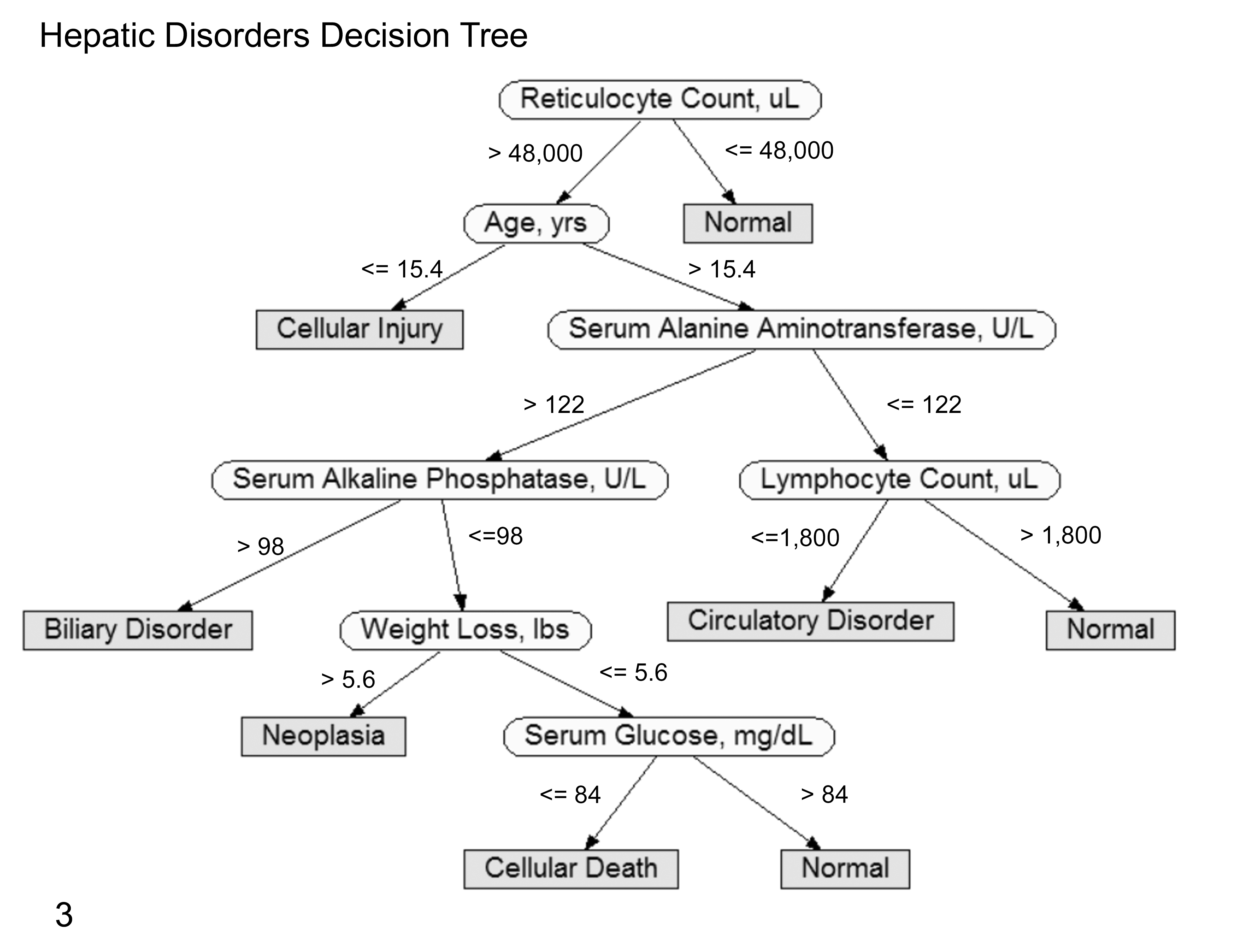
Graphical depiction of a decision tree using various laboratory and clinical data to predict 5 hepatic disorders generated by the C4.5 classifier (WEKA, Machine Learning Group at the University of Waikato, Hamilton, New Zealand). Classification or disorder nodes are rectangular/gray and located at the end of tree branches (leaves of the tree). Decision evidence nodes are oval/unshaded. Numeric values shown are used for deciding the branching direction at a decision node. These values are established by a learning algorithm to maximize disorder classification accuracy using historic data. For predicting the disorder classification of a new case, findings for the evidence nodes are considered in sequence as shown by the tree (top down) to arrive at the favored disorder node. Unlike Bayesian networks, the disorder predictions are yes/no with a single positive outcome for each case considered.

A classification tree creates a hierarchical data structure composed of nodes; the first node on the tree is called the root node, and then subsequent child nodes are referred to as internal nodes. Each of these internal nodes represents a particular test used to classify instances (eg, “Is the patient male or female?”). For each possible outcome of a test, a child node is present. In cases of discrete attributes, an attribute A has h possible outcomes A = d ₁…d_h , where d ₁…d_h are known A attribute values. In a case of a continuous attribute, there are 2 possible outcomes: A ≤ t or A > t, where t is a value of a threshold that is to be determined at the node. The nodes at the end of the tree are termed leaf nodes, and they are used to identify the class to which the case instance will be assigned (eg, “patient with cancer”). Decision tree classification techniques are embodied in packages, such as CART, ID3, and C4.5.^17,80,83

The C4.5 decision tree classifier is recognized for its user-friendly structure. It provides a tree that is easy to use at the point of practice and allows the user to see its underlying logic. Unlike with naive Bayes classifiers, decision trees do not assume independencies between attributes, making them applicable in many scenarios. Previous studies have shown the C4.5 classifier worked well in dealing with problems related to traffic management, marketing, health insurance industry, gene identification, and medical diagnoses.^{7,44,47,49,60,71,111,119}

Artificial Neural Network

In the 1940s, a study reported computational models that represent biological neural networks mathematically.¹¹⁰ Interested groups then used these neural network models to represent biological processes in the nervous system and to model artificial intelligence. Scientists have shown that neural networks can mathematically model neuron biological structure, memory function, and knowledge storage and retrieval.^64,82

In artificial neural network algorithms, knowledge is acquired through a learning process called backpropagation and stored within the interconnection strength (weights) between neurons (called nodes). Developers can build such algorithms out of single-layer neurons (called single-layer perceptron) or neurons arranged in multiple layers (multilayer perceptron). While single-layer perceptron algorithms classify instances into categories using direct relationships between input and output nodes, they cannot be used to solve every problem. Some sets of instances cannot be divided into distinct categories by a simple linear relationship. Multilayer perceptron algorithms with more than 1 layer of neurons were developed to deal with more complex nonlinear scenarios.

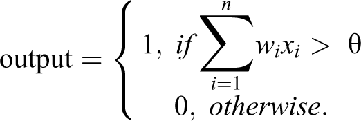
For illustration, a single-layer perceptron with x₁ …x_n input layer attributes, and with y as the class attribute (output layer) of data set D, has w₁ …w_n weights for the relationships between the input and the output nodes. These weights are adjusted based on outcome accuracy learned from previous instances (Fig. 4). The single-layer perceptron algorithm then classifies new instances given their input attribute values, where θ is a threshold value designated to make a classification to a particular output node, that is,

Figure 4.

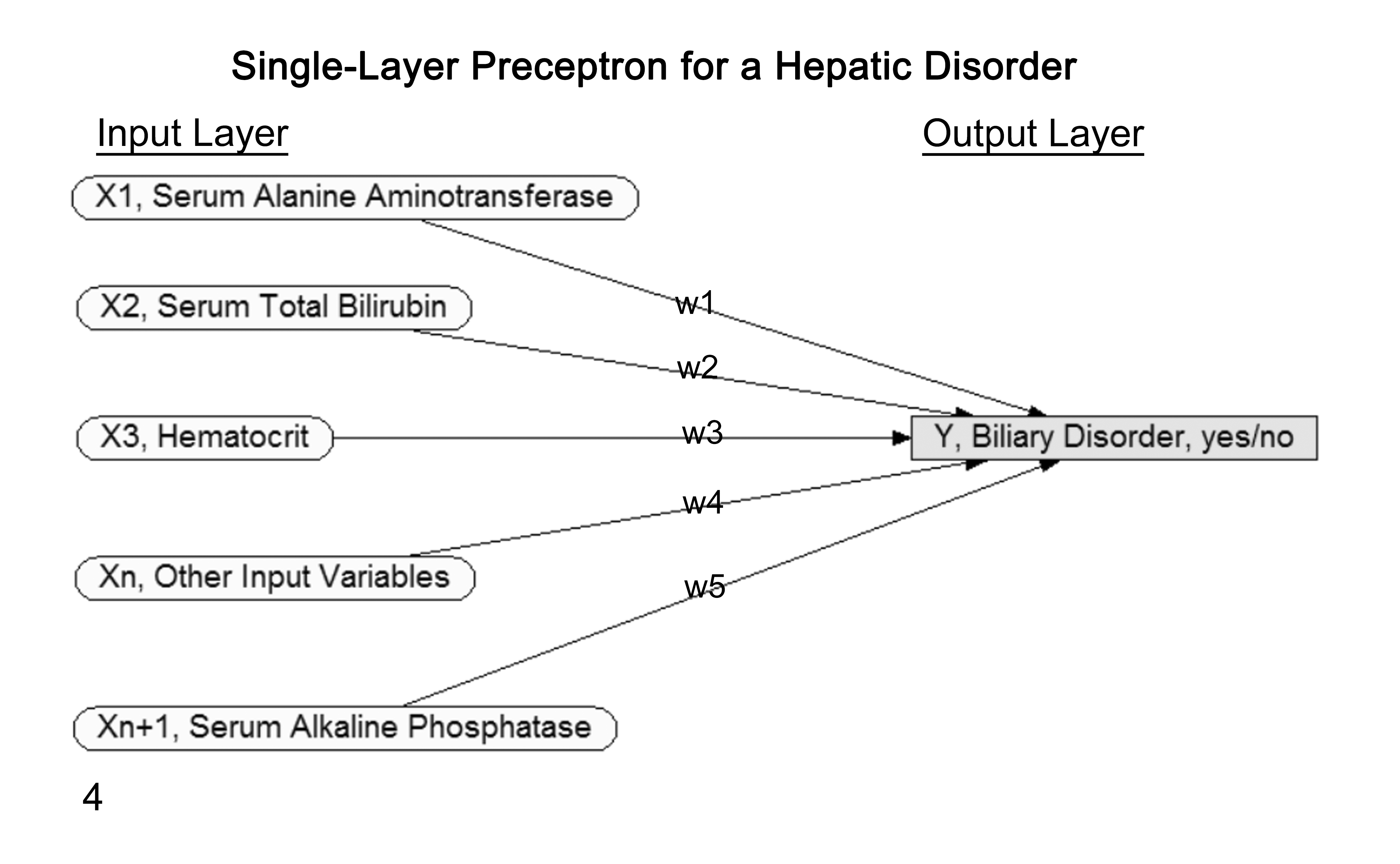
Graphical depiction of a single-layer perceptron neural network for a single hepatic disorder. The rectangular/gray output disorder “Y” node is on the far right. The oval/unshaded input “X_{1 – n}” evidence nodes are on the far left, with “n” representing the number of evidence nodes used in the network. The “w_1–5” represent the individual weighting values assigned for each evidence node’s influence on the state of the output disorder node. The weights are learned by the network to maximize the disorder’s status (yes/no) accuracy using historic data. For predicting status of a new case, findings for the evidence nodes are considered in light of established weights to calculate the disorder node’s state. This general approach is repeated for each specific disorder of interest.

output = {\begin{matrix} 1, i f \sum_{i = 1}^{n} w_{i} x_{i} > θ \\ 0, o t h e r w i s e . \end{matrix}

In contrast, a multilayer perceptron includes 1 or more “hidden” layers composed of nodes h₁ …h_n placed between the input and output nodes (Fig. 5). Unlike with the single-layer perceptron, multilayer perceptron models have the ability to train the hidden nodes by adjusting their weights. This weight adjusting is most commonly done through a process called backpropagation.⁴⁰ This method was introduced in 1986 to repeatedly adjust the weights of the connections in the network with the goal of minimizing the difference between predicted network output and the true status of the case.¹¹⁰

Figure 5.

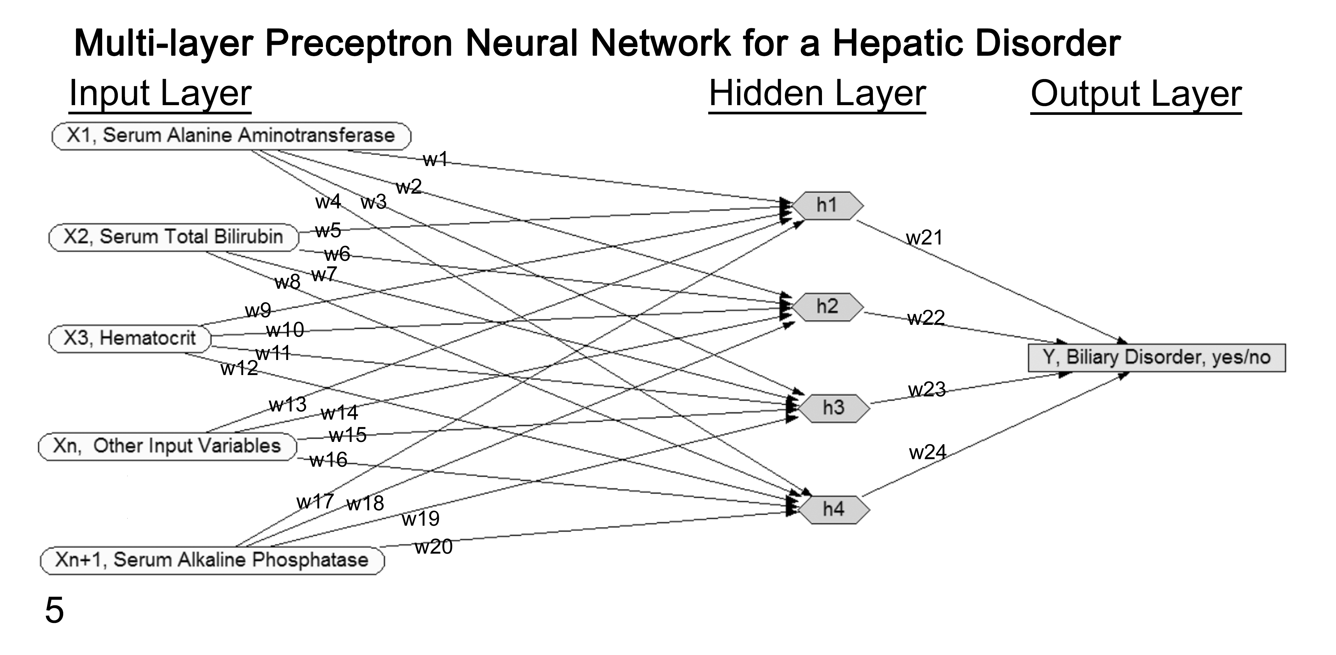
Diagram of a multilayer perceptron neural network for a single hepatic disorder. The rectangular/gray output disorder “Y” node is on the far right. The oval/unshaded input “X_{1 – n}” evidence nodes are on the far left, with “n” representing the number of evidence nodes used in the network. The “w_1–24” represent the individual weighting values assigned for each node’s influence on the state of the output disorder node. The weights are learned by the network to maximize the disorder’s status accuracy (yes/no) using historic data. The “hidden layer” of hexagon/gray nodes is a distinguishing feature of a multilayer network. The user has no direct interaction with these nodes, but they allow the network to solve more complex problems. Values for these hidden nodes are auto-assigned by one of several possible learning algorithms using historic data to maximize the disorder’s status accuracy. For predicting status of a new case, findings for the evidence nodes are considered in light of established weights and hidden node values to calculate the disorder node’s state. This general approach is repeated for each specific disorder of interest.

Since multilayer perceptron networks use “hidden” layers of nodes to arrive at their classifications, justification for the results can be difficult for users to understand. For this reason, the term black box is commonly associated with multilayer perceptron algorithms. Despite this opaqueness, multilayer perceptron neural networks may be able to solve scenarios that decision tree and naive Bayes algorithms cannot.^{33,66,71,101,106}

With understanding of these 3 basic learning algorithms, we will next explore some of the common steps involved in the preparation and validation of patient data sets for use with these tools.

Data Sets

Regardless of the decision support tool being used or its underlying learning algorithm, they all are dependent upon input data to arrive at their classification predictions. It has been shown that the quality of these input data has a high impact on the machine-learning process and performance of these systems.^24,93 Therefore, data preparation and use for training often consume the bulk of effort associated with use of decision support tools in medicine. In this section, we explore some of the basic topics associated with optimizing these data and their use for validating classifier performance.

Storage

Machine learning extracts knowledge from computable information. This information can be considered a set of instances (individual cases), and these instances are then used for training and testing the prediction models. In most preprocessing situations, instances are stored in an independent and nonredundant relational database. In every relation (table), rows are instances and columns are features (attributes) that represent variables to be recorded for every instance. The feature values can be numeric, nominal, images, sounds, or others. However, all data are transformed into numerical values for computational efficiency as an early preprocessing step.

Transformation and Free-Text Preprocessing

Data transformation is the method of converting data values from the source format into an input format to be processed. Successful machine learning involves more than simply selecting a particular learning algorithm. Most algorithms have various parameters and value settings that influence performance and the transformation of input data. Studies have shown that prediction results can be improved if developers optimize these value settings. For example, discretization (ie, transforming continuous functions into discrete counterparts) is one of the most common data transformation methodologies. Discretization or binning has received a great deal of attention in the data mining community, and there are multiple methods (eg, equal interval, equal frequency, and entropy based).^18,29,118 Moreover, there are classifiers that are called discrete classifiers, which take discrete values to achieve improved performance; a decision tree is an example of a discrete classifier that is very commonly used.¹⁹

Machine-learning algorithms are frequently used to extract information from free text. Various transformation methodologies have been developed to render free-text documents in a more computationally friendly format. A “Bag of Words” is one such example in which each individual document being considered is represented by a set of words (called features) that are extracted from its text.^70,90 Frequency of occurrences of all words within the bag and across other bags can be used as quantitative measurements to represent the content of each document. Another study evaluated the effect of transforming free text into a vector of numerical descriptors.⁴⁶ The study reviewed techniques such as term frequency (frequency of a term in a document), term frequency with inverse document frequency (in which terms that appear in all documents are overlooked), and term frequency with inverse class frequency (in which terms are weighted according to their relationship with document categories or classes). Results of this study showed that the term frequency with inverse document frequency and inverse class frequency weighting factors either improved or did not change performance of the classifiers.

Different methodologies have been examined for optimizing the extracted set of words used to represent the class of each document. Among these methodologies is text tokenization, also called text segmentation. In this approach, the text is divided into meaningful units presented as words, sentences, or topics.²¹ Text segmentation focuses on extracting alphabetical content from the text corpus and ignores any nonalphabetical content. Word stemming is another technique that has shown to have a positive impact on free-text analysis.^46,85,97 In stemming, words are reduced to their stems or roots so that words with similar roots may be gathered together. Stemming usually results in the removal of derivational suffices and prefixes (affixes), with the assumption that similar roots are synonyms. In a 2015 study, researchers found that stemming reduced the set of features, or attributes values, to be considered in a free-text document from 9793 to 936 with little impact on classifier accuracy.²⁹

Representation of free text using taxonomies (controlled terminology) has also been used as a preprocessing step. This rendering results in abstracting the concepts of the original document in a standardized format. This methodology has the advantage of identifying related concepts (such as synonyms) without having to explicitly declare them individually. The successful use of taxonomy concept abstraction in conjunction with “bag-of-words” feature selection has been demonstrated.¹¹³ Moreover, the use of taxonomy categories adds new information that is not conveyed by the free text within the corpus. Depending upon taxonomy used, concept meaning can be inferred by hierarchal location and by explicit and implicit relationships in the hierarchy itself (eg, “neutrophilic inflammation-concept is a-relationship” type of “inflammation-concept”).^11,87 Furthermore, use of these terminologies facilitates the efficient retrieval and analysis of coded documents. There are several studies examining the use of taxonomy concepts and machine-leaning techniques to formulate evidence-based guidelines, syndromic disease surveillance, disease detection, and case retrieval.^5,6,9,35

Another preprocessing step shown to improve learning from free text is excluding a list of words not dependent on a class or topic. A list of words called “stop words” is excluded from being considered in the “bag of words” to improve tokenization accuracy and speed.⁸¹ For example, literature has shown that the word the appears in almost all documents, accounts for a large percentage of the words, and has no relevance to any particular category or class when learning. Therefore, it is advantageous to exclude the word the before preparing the data for input. A recent study showed that stop words counted for 9% of the extracted text features and, therefore, hamper the effort of learning by machines and introduce unnecessary additional complexity.⁹³

Feature Selection

Previous studies have shown that a learning algorithm’s performance can be negatively affected by training with data sets that have too many features or attributes. In these cases, the decision support tools can be described as becoming overfitted to the training data and then fail to perform well with new real-world scenarios. To guard against this risk, developers select a subset of variables from the data set in a process called feature selection.

The number of words extracted from a free-text document of moderate length can easily reach 10,000 words.^16,90 There is also the tendency for investigators to gather as much data as possible (ie, “more is better”). However, in machine learning, this may or may not be true. There is evidence that machine-learning algorithms do better when subsets of features are selected for learning.^16,39,75 Irrelevant or redundant data can negatively affect the performance of the computational models by adding noise. This effect can increase the algorithm runtime, introduce more complexity (results are harder to interpret), and overfit the training data set.⁵⁶

A study conducted in 2010 compared the effect of threshold-based feature selection techniques on 3 different models. Authors evaluated the impact of different feature selection methodologies using 8 different metrics: area under the curve (AUC), precision-recall plot, default F-measure (corresponds to a decision threshold value of 0.5), best F-measure (the largest value of F-measure when varying the decision threshold value between 0 and 1), default geometric mean, best geometric mean, default arithmetic mean, and best arithmetic mean.¹⁰⁵ The study found that the prediction performance of the models either improved or remained unchanged despite removal of 96% of the features used as input; in fact, they found that in 95% of the cases, results were improved. Similarly, in another 2013 study, authors examined the effect of feature selection methodologies on machine-learning performance for 5 algorithms: Trees.J45, Bayes.BayesNet, Functions.Logestic, Meta.Bagging, and Rules.ZeroR.⁵⁵ Authors found that when the number of input features was reduced by 75%, classification performance improved or remained the same. They also concluded that the performance depended most on the specific features selected in the subset and was independent of the actual number.

Filters and wrappers are 2 more methodologies for selecting the best relevant features prior to classification. These 2 techniques have been shown to significantly improve the performance of the prediction models.³⁹ In the filter approach, any features not correlated to one of the class labels are filtered out based on some general characteristics of the training data, such as statistical dependencies. This approach is considered faster than wrapper because it acts independently from the induction algorithm (the algorithm that is used evaluates each subset). However, this approach tends to select a higher number of features than may be optimal.⁶³ In wrapper, a subset of features is selected as part of the algorithm and tailored to a particular learning application. Unlike with the filter approach, wrapper uses an induction algorithm as part of the evaluation process of different feature subsets. The wrapper algorithm searches for features that best suit the machine-learning algorithm used for prediction, and this makes it more computationally expensive than the filter method.⁵¹

Several other search methods have been developed to help reduce the number of features within the data set. Most of these methods search for the set of attributes that is most likely to predict the class. “Greedy” searching of the space is one such method. With a greedy search algorithm, the data set space is searched either forward or backward by adding or removing a single attribute at each step. The forward direction starts with no attributes and then adds one at a time. The backward elimination starts with all attributes and deletes one at a time. With the greedy approach feature, adding or removing stops when the classification performance of the learning algorithm drops. Another search-type method is best-first, in which the search does not stop when the performance of the new data set declines.⁵³ Instead, with best-first, the searching method continues to look for new subsets while keeping the old ones in the memory, then sorts subsets by their performance measurements. The best-first algorithm is considered more computationally expensive as a result of these memory and time requirements. However, this methodology assesses the entire space of attributes to guarantee selection of the best subset, and it has been shown to be very effective.¹¹¹ In a 2011 study using a machine-learning algorithm to identify brain neoplasms from MRI, authors evaluated performance effects of using best-first, greedy stepwise, K-nearest neighbor, and scatter methods for feature selection/reduction.¹¹⁶ The authors found that using the K-nearest neighbor wrapper in combination with best-first algorithm resulted in the highest classification accuracy. In another 2011 study using patients with Alzheimer disease and single-photon emission computed tomography data, classification models were built to distinguish between healthy and diseased cohorts. The classification performance of these models improved following use of techniques like bootstrap resampling, spatial normalization, smoothing, intensity normalization, multivariate image analysis based on principal component analysis, and Fisher discriminant analysis.⁶⁵ The particular importance of feature selection/reduction is made clear by these last 2 studies in light of the inherent complexity of image data. In most image analysis studies, patterns are extracted from images using pattern recognition filters. These complex patterns are abstracted as a large collection of numerical attributes, which is then reduced by one of the previously discussed features section methods (eg, principal component analysis).

Testing

In most of the decision support systems discussed, machine learning is based on the use of previous instances to train the supervised classifier. After training, the classifier is then tested for its ability to predict the class (dependent variable) of a new case given the values of its attributes (independent variables). Usually, the classifier’s performance is evaluated with a data set that was not used for training; this is done to provide a prospective view of how the classifier will perform with new cases. There are 2 common ways of splitting a data set: simple-random and cross-validation.

In the first technique, simple-random, the data set is divided based on a particular percentage, such as 60% used for training and 40% used for testing. Some studies used 50% for training and 50% for testing; others chose to split into 70% training and 30% testing.^38,55,72 Authors of 1 study challenged the classifier after using less than 10% of instances for training.¹¹⁵ In this study, the researchers found that training a naive Bayes algorithm on 10% of the instances and testing with 90% resulted in 95.20% accuracy and an F-measure value of over 97%. While the exact percentage varies, most studies agree that the optimal division is to use 60% to 80% of instances for training and to test performance with the reminder.

Cross-validation is another common approach to splitting a data set for training and testing. Unlike simple-random splits, cross-validation uses all instances in training by performing multiple rounds of divisions using different training subsets, which collectively covers all instances (Fig. 6). Commonly, multiple rounds of cross-validation are performed, and performance results from the rounds or folds are averaged to reduce variability.^26,50 There are several cross-validation approaches based on the number of folds (rounds) selected. The most common approach is K-fold cross-validation, where K is the number of folds to be created with K = 10 being the most common. Leave-P-out cross-validation is another approach, in which P is equal to the number of instances used in testing and the rest used in training. Leave-one-out cross-validation is another common approach that represents K-fold cross-validation taken to its extreme, with K equal to the number of instances in the data set.

Figure 6.

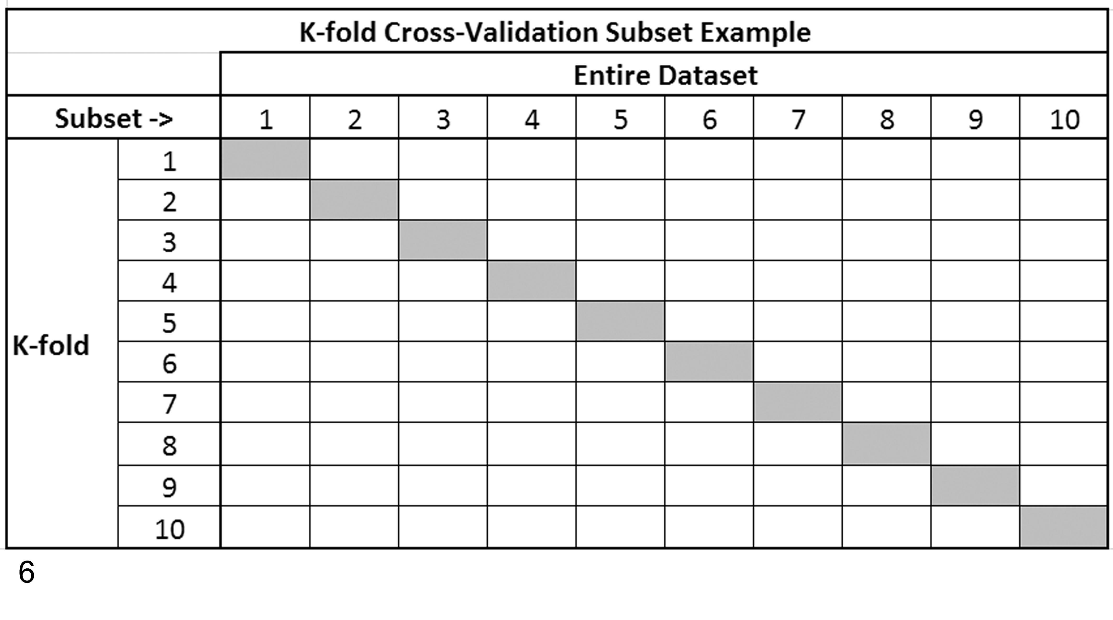
A 10-fold cross-validation example of subsetting a data set for purposes of creating portions for training (gray) and portions for testing (white) a machine-learning algorithm. K represents the number of folds (iterations) of training and testing the algorithm, with each fold using a different portion of the data set until all instances have been used for both purposes. Overall classification prediction performance for the algorithm being evaluated would be determined from the averaged results from each of the 10-folds shown in the example.

Regardless of the exact method used to split out the testing data set, it is then used to access sensitivity, specificity, and accuracy of class predictions for the learning algorithm being examined.

Conclusion

Extensive research and work have been done to develop computer-based decision support tools to assist clinicians across many facets of patient care. A general thesis put forth by developers of these systems is that these applications improve the accuracy of medical diagnoses and contribute to better patient outcomes. Through this review, we have presented supporting evidence for the former but less so for the latter, which is a harder assessment end point to study. With increased deployment of these tools in veterinary pathology, we hope more evidence-based outcome assessments will become available. Another general premise of these tools is that they are not intended to replace health care experts but to support their work and position them as information managers. Specifically, these tools are envisioned to support ad hoc decision making as expressed by the concept of “human-assisted computer diagnosis.”⁶⁸ As pathologists and medical decision makers in the age of these tools, basic understanding of their functionality is fast becoming part of the standard of care owed to our patients.

Footnotes

Declaration of Conflicting Interests

The author(s) declared no potential conflicts of interest with respect to the research, authorship, and/or publication of this article.

Funding

The author(s) received no financial support for the research, authorship, and/or publication of this article.

ORCID iD

Kurt L. Zimmerman

References

Abbass

. An evolutionary artificial neural networks approach for breast cancer diagnosis. Artif Intell Med. 2002;25(3):265–281.

Abbod

Catto

Linkens

, et al. Application of artificial intelligence to the management of urological cancer. J Urol. 2007;178(4):1150–1156.

Al-Kadi

. A multiresolution clinical decision support system based on fractal model design for classification of histological brain tumours. Comput Med Imaging Graph. 2015;41:67–79.

Al-Omari

Matalka

Al-Jarrah

, et al. An intelligent decision support system for quantitative assessment of gastric atrophy. J Clin Pathol. 2011;64(4):330–337.

Anholt

Berezowski

Jamal

, et al. Mining free-text medical records for companion animal enteric syndrome surveillance. Prev Vet Med. 2014;113(4):417–422.

Anholt

Berezowski

Maclean

, et al. The application of medical informatics to the veterinary management programs at companion animal practices in Alberta, Canada: a case study. Prev Vet Med. 2014;113(2):165–174.

Araújo

Santana

, Neto PdAS. Using machine learning to support healthcare professionals in making preauthorisation decisions. Int J Med Inform. 2016;94:1–7.

Arevalo

Cruz-Roa

Arias

, et al. An unsupervised feature learning framework for basal cell carcinoma image analysis. Artif Intell Med. 2015;64(2):131–145.

Arsevska

Roche

Hendrikx

, et al. Identification of terms for detecting early signals of emerging infectious disease outbreaks on the web. Comput Electron Agric. 2016;123:104–115.

10.

Awaysheh

Wilcke

Elvinger

, et al. Identifying free-text features to improve automated classification of structured histopathology reports for feline small intestinal disease. J Vet Diagn Invest. 2018;30(2):211–217.

11.

Awaysheh

Wilcke

Elvinger

, et al. A review of medical terminology standards and structured reporting. J Vet Diagn Invest. 2018;30(1):17–25.

12.

Awaysheh

Wilcke

Elvinger

, et al. Evaluation of supervised machine-learning algorithms to distinguish between inflammatory bowel disease and alimentary lymphoma in cats. J Vet Diagn Invest. 2016;28(6):679–687.

13.

Barnett

Cimino

Hupp

, et al. DXplain: experience with knowledge acquisition and program evaluation. In: Proceedings of the Annual Symposium on Computer Application in Medical Care. Washington, DC: American Medical Informatics Association; 1987:150–154.

14.

Bishop

. Pattern Recognition and Machine Learning. New York, NY: Springer; 2006.

15.

Blois

Tuttle

Sherertz

. RECONSIDER: a program for generating differential diagnoses. In: Proceedings of the Annual Symposium on Computer Application in Medical Care. Washington, DC: American Medical Informatics Association; 1981:263–268.

16.

Blum

Langley

. Selection of relevant features and examples in machine learning. Artif Intell. 1997;97(1):245–271.

17.

Breiman

. Classification and Regression Trees. Belmont, CA: Wadsworth; 1984.

18.

Butterworth

Simovici

Santos

, et al. A greedy algorithm for supervised discretization. J Biomed Inform. 2004;37(4):285–292.

19.

Canisius

van den Bosch

Daelemans

. Discrete versus probabilistic sequence classifiers for domain-specific entity chunking. In: Proceedings of the Eighteenth Belgian-Dutch Conference on Artificial Intelligence (BNAIC-2006). Namur, Belgium: Benelux Artificial Intelligence Conference; 2006:1–8.

20.

Cannon

Allen

. A comparison of the effects of computer and manual reminders on compliance with a mental health clinical practice guideline. J Am Med Inform Assoc. 2000;7(2):196–203.

21.

Choi

. Advances in domain independent linear text segmentation. In: Proceedings of the 1st North American Chapter of the Association for Computational Linguistics Conference. Seattle, WA: The North American Chapter of the Association for Computational Linguistics; 2000:26–33.

22.

Christopher

Hotz

. Cytologic diagnosis: expression of probability by clinical pathologists. Vet Clin Pathol. 2004;33(2):84–95.

23.

Cosma

Acampora

Brown

, et al. Prediction of pathological stage in patients with prostate cancer: a neuro-fuzzy model. PLoS One. 2016;11(6):e0155856.

24.

Crone

Lessmann

Stahlbock

. The impact of preprocessing on data mining: an evaluation of classifier sensitivity in direct marketing. Eur J Oper Res. 2006;173(3):781–800.

25.

Dheeba

Tamil Selvi

. An improved decision support system for detection of lesions in mammograms using differential evolution optimized wavelet neural network. J Med Syst. 2012;36(5):3223–3232.

26.

Dietterich

. Machine-learning research: four current directions. AI Mag. 1997;18(4):97–136.

27.

Domingosm

Pazzani

. Beyond independence: conditions for the optimality of the simple Bayesian classifier. In: Proceedings of the 13th International Conference on Machine Learning. Bari, Italy: International Conference on Machine Learning; Bari, Italy: International Conference on Machine Learning; 1996:105–112.

28.

Dórea

Muckle

Kelton

, et al. Exploratory analysis of methods for automated classification of laboratory test orders into syndromic groups in veterinary medicine. PLoS One. 2013;8(3):e57334.

29.

Dougherty

Kohavi

Sahami

. Supervised and unsupervised discretization of continuous features. In: Machine Learning: Proceedings of the Twelfth International Conference. Tahoe, CA: International Conference on Machine Learning; 1995:194–202.

30.

Evans

Pestotnik

Classen

, et al. A computer-assisted management program for antibiotics and other antiinfective agents. N Engl J Med. 1998;338(4):232–238.

31.

Faria

Costa

Giusta

, et al. High-throughput analysis of synthetic peptides for the immunodiagnosis of canine visceral leishmaniasis. PLoS Negl Trop Dis. 2011;5(9):e1310.

32.

Faunt

Lund

Novak

. The power of practice: harnessing patient outcomes for clinical decision making. Vet Clin North Am Small Anim Pract. 2007;37(3):521–532.

33.

Ferreira

Oliveira

Freitas

. Applying data mining techniques to improve diagnosis in neonatal jaundice. BMC Med Inform Decis Making. 2012;12(1):1.

34.

Floyd

Yun

, et al. Prediction of breast cancer malignancy using an artificial neural network. Cancer. 1994;74(11):2944–2948.

35.

Furrer

Küker

Berezowski

, et al. Constructing a syndromic terminology resource for veterinary text mining. In: Proceedings of the Conference Terminology and Artificial Intelligence. Granada, Spain: The Spanish Society for Applied Linguistics; 2015:61–70.

36.

Furundzic

Djordjevic

Bekic

. Neural networks approach to early breast cancer detection. J Syst Architect. 1998;44(8):617–633.

37.

Garg

Adhikari

McDonald

, et al. Effects of computerized clinical decision support systems on practitioner performance and patient outcomes: a systematic review. JAMA. 2005;293(10):1223–1238.

38.

Gramatica

Pilutti

Papa

. Validated QSAR prediction of OH tropospheric degradation of VOCs: splitting into training-test sets and consensus modeling. J Chem Inf Comput Sci. 2004;44(5):1794–1802.

39.

Hall

Smith

. Feature subset selection: a correlation based filter approach. In: International Conference on Neural Information Processing and Intelligent Information Systems. Dunedin/Queenstown, New Zealand: International Conference on Neural Information Processing; 1997:855–858.

40.

Haykin

. Neural Networks and Learning Machines. Upper Saddle River, NJ: Pearson; 2009.

41.

Hills

Kulbok

Clark

. Evaluating a quality improvement program for cervical cancer screening at an urban safety net clinic. Health Promot Pract. 2015;16(5):631–641.

42.

Hunt

Marin

Stone

. Experiments in Induction. New York, NY: Academic Press; 1966.

43.

Hutchings

. How does PET/CT help in selecting therapy for patients with Hodgkin lymphoma? ASH Educat Program Book. 2012;2012(1):322–327.

44.

Ichikawa

Saito

Ujita

, et al. How can machine-learning methods assist in virtual screening for hyperuricemia? A healthcare machine-learning approach. J Biomed Inform. 2016:64:20–24.

45.

Jimbo

Rana

Hawley

, et al.

What is lacking in current decision aids on cancer screening?

CA Cancer J Clin. 2013;63(3):193–214.

46.

Jouhet

Defossez

Burgun

, et al. Automated classification of free-text pathology reports for registration of incident cases of cancer. Methods Inf Med. 2012;51(3):242–251.

47.

Jowkar

Mansoori

. Perceptron ensemble of graph-based positive-unlabeled learning for disease gene identification. Comput Biol Chem. 2016;64:263–270.

48.

Julia-Sape

Majos

Camins

, et al. Multicentre evaluation of the INTERPRET decision support system 2.0 for brain tumour classification. NMR Biomed. 2014;27(9):1009–1018.

49.

Karim

Rahman

. Decision tree and naive Bayes algorithm for classification and generation of actionable knowledge for direct marketing. Int J Eng Res Appl. 2013;6(4):196–206.

50.

Kohavi

. A study of cross-validation and bootstrap for accuracy estimation and model selection. IJCAI. 1995;2:1137–1145.

51.

Kohavi

John

. Wrappers for feature subset selection. Artif Intell. 1997;97(1):273–324.

52.

Kononenko

. Machine learning for medical diagnosis: history, state of the art and perspective. Artif Intell Med. 2001;23(1):89–109.

53.

Korf

. Linear-space best-first search. Artif Intell. 1993;62(1):41–78.

54.

Kullback

Leibler

. On information and sufficiency. Ann Stat 1951;22(1):79–86.

55.

Kwon

Rhee

Yoon

. Application of classification algorithms for analysis of road safety risk factor dependencies. Accid Anal Prev. 2015;75:1–15.

56.

Langley

. Selection of relevant features and examples in machine learning. Artif Intell. 1997;97(1–2):245–271.

57.

Laton

Van Schependom

Gielen

, et al. Single-subject classification of schizophrenia patients based on a combination of oddball and mismatch evoked potential paradigms. J Neurol Sci. 2014;347(1–2):262–267.

58.

Ledley

Lusted

. Reasoning foundations of medical diagnosis. Science New Series. 1959;130(3366):9–21.

59.

Lewis

Sharp

Bartholomew

, et al. Computerized assessment of common mental disorders in primary care: effect on clinical outcome. Fam Pract. 1996;13(2):120–126.

60.

Liao

Huang

Yue

, et al. In silico prediction of gamma-aminobutyric acid type—a receptors using novel machine-learning-based SVM and GBDT approaches. Biomed Res Int. 2016;2016:2375268.

61.

Lindley

Gillies

Hassell

. Communicating diagnostic uncertainty in surgical pathology reports: disparities between sender and receiver. Pathol Res Pract. 2014;210(10):628–633.

62.

Lipkin

Hardy

. Mechanical correlation of data in differential diagnosis of hematological diseases. J Am Med Assoc. 1958;166(2):113–125.

63.

Liu

. Toward integrating feature selection algorithms for classification and clustering. IEEE Trans Knowl Data Eng. 2005;17(4):491–502.

64.

McCulloch

Pitts

. A logical calculus of the ideas immanent in nervous activity. Bull Math Biophys. 1943;5(4):115–133.

65.

Merhof

Markiewicz

Platsch

, et al. Optimized data preprocessing for multivariate analysis applied to 99mTc-ECD SPECT data sets of Alzheimer’s patients and asymptomatic controls. J Cereb Blood Flow Metab. 2011;31(1):371–383.

66.

Mert

Kilic

Bilgili

, et al. Breast cancer detection with reduced feature set. Comput Math Methods Med 2015;2015:265138.

67.

Miller

. INTERNIST-l/CADUCEUS: problems facing expert consultant. Meth Inform Med. 1984;23(1):9–14.

68.

Miller

. Why the standard view is standard: people, not machines, understand patients’ problems. J Med Philos. 1990;15(6):581–591.

69.

Miller

McNeil

Challinor

, et al. The INTERNIST-1/quick medical REFERENCE project—status report. West J Med. 1986;145(6):816–822.

70.

Needham

. Organizing Knowledge in Libraries: An Introduction to Information Retrieval. London, UK: Andre Deutsch; 1971.

71.

Palaniappan

Awang

. Intelligent heart disease prediction system using data mining techniques. In: 2008 IEEE/ACS International Conference on Computer Systems and Applications. Doha, Qatar: Institute of Electrical and Electronics Engineers; 2008:108–115.

72.

Pankratz

Degnim

Frank

, et al. Model for individualized prediction of breast cancer risk after a benign breast biopsy. J Clin Oncol. 2015;23(8):923–929.

73.

Parkhi

Vedaldi

Jawahar

, et al. The truth about cats and dogs. In: 2011 International Conference on Computer Vision. Barcelona, Spain: Institute of Electrical and Electronics Engineers; 2011:1427–1434.

74.

Parkhi

Vedaldi

Zisserman

, et al. Cats and dogs. In: 2012 IEEE Conference on Computer Vision and Pattern Recognition (CVPR). Providence, RI: Institute of Electrical and Electronics Engineers; 2012:3498–3505.

75.

Piramuthu

. Evaluating feature selection methods for learning in data mining applications. Eur J Oper Res. 2004;156(2):483–494.

76.

Pople

Myers

Miller

. DIALOG: a model of diagnostic logic for internal medicine. IJCAI. 1975;1:848–855.

77.

Pozen

D’Agostino

Selker

, et al. A predictive instrument to improve coronary-care-unit admission practices in acute ischemic heart disease: a prospective multicenter clinical trial. N Engl J Med. 1984;310(20):1273–1278.

78.

Prasad

Bruce

Ball

JE.

A multi-classifier and decision fusion framework for robust classification of mammographic masses. In: 2008 30th Annual International Conference of the IEEE Engineering in Medicine and Biology Society. Vancouver, Canada: Institute of Electrical and Electronics Engineers; 2008:3048–3051.

79.

Qiu

Shimada

Hiraoka

, et al. Knowledge discovery for pancreatic cancer using inductive logic programming. IET Syst Biol. 2014;8(4):162–168.

80.

Quinlan

. Induction of decision trees. Machine Learn. 1986;1:81–106.

81.

Reynar

. Topic segmentation: algorithms and applications. 1998. https://repository.upenn.edu/cgi/viewcontent.cgi?%20article=1068&context=ircs_reports. Accessed February 8, 2017.

82.

Rosenblatt

. The perceptron: a probabilistic model for information storage and organization in the brain. Psychol Rev. 1958;65(6):386–408.

83.

Salzberg

. C4. 5: Programs for machine learning. Machine Learn. 1994;16(3):235–240.

84.

Santamaria

Zimmerman

. Uses of informatics to solve real world problems in veterinary medicine. J Vet Med Educ. 2011;38(2):103–109.

85.

Savoy

. A stemming procedure and stopword list for general French corpora. J Assoc Inf Sci Technol. 1999;50(10):944–952.

86.

Sawka

Straus

Rodin

, et al. Decision aid on radioactive iodine treatment for early stage papillary thyroid cancer: update to study protocol with follow-up extension. Trials. 2015;16:302.

87.

Schadow

McDonald

. Extracting structured information from free text pathology reports. AMIA Annu Symp Proc. 2003;2003:584–588.

88.

Schmickl

Pannu

Al-Qadi

, et al. Decision support tool for differential diagnosis of acute respiratory distress syndrome (ARDS) vs cardiogenic pulmonary edema (CPE): a prospective validation and meta-analysis. Crit Care. 2014;18(6):659.

89.

Schriger

Gibbons

Langone

, et al. Enabling the diagnosis of occult psychiatric illness in the emergency department: a randomized, controlled trial of the computerized, self-administered PRIME-MD diagnostic system. Ann Emerg Med. 2001;37(2):132–140.

90.

Sebastiani

. Machine learning in automated text categorization. ACM Comput Surv. 2002;34(1):1–47.

91.

Selker

Beshansky

Griffith

, et al. Use of the acute cardiac ischemia time-insensitive predictive instrument (ACI-TIPI) to assist with triage of patients with chest pain or other symptoms suggestive of acute cardiac ischemia: a multicenter, controlled clinical trial. Ann Intern Med. 1998;129(11, pt 1):845–855.

92.

Setiono

. Extracting rules from pruned neural networks for breast cancer diagnosis. Artif Intell Med. 1996;8(1):37–51.

93.

Sharma

Jain

. Evaluation of stemming and stop word techniques on text classification problem. Int J Scientific Res Comp Sci Eng. 2015;3(2):1–4.

94.

Shen

Colloc

Jacquet-Andrieu

Lei

. Emerging medical informatics with case-based reasoning for aiding clinical decision in multi-agent system. J Biomed Inform. 2015;56:307–317.

95.

Shortliffe

Buchanan

Feigenbaum

. Knowledge engineering for medical decision making: a review of computer-based clinical decision aids. Proceed IEEE. 1979;67(9):1207–1224.

96.

Simões

Izumi

Casagrande

, et al. Classification of images acquired with colposcopy using artificial neural networks. Cancer Inform. 2014;13:119–125.

97.

Spasic

Livsey

Keane

, et al. Text mining of cancer-related information: review of current status and future directions. Int J Med Inform. 2014;83(9):605–623.

98.

Stewart

Shah

Selna

, et al. Bridging the inferential gap: the electronic health record and clinical evidence. Health Aff (Millwood). 2007;26(2):w181–w191.

99.

Tsolaki

Svolos

Kousi

, et al. Fast spectroscopic multiple analysis (FASMA) for brain tumor classification: a clinical decision support system utilizing multi-parametric 3 T MR data. Int J Comput Assist Radiol Surg. 2015;10(7):1149–1166.

100.

Uguz

. A biomedical system based on artificial neural network and principal component analysis for diagnosis of the heart valve diseases. J Med Syst. 2012;36(1):61–72.

101.

Venkatasubramanian

King

. A neural network methodology for process fault diagnosis. AIChE J. 1989;35(12):1993–2002.

102.

Verma

Srivastava

Negi

. A hybrid data mining model to predict coronary artery disease cases using non-invasive clinical data. J Med Syst. 2016;40(178):1–7.

103.

Wagholikar

MacLaughlin

Henry

, et al. Clinical decision support with automated text processing for cervical cancer screening. J Am Med Inform Assoc. 2012;19(5):833–839.

104.

Wan

Bao

. Animal disease diagnoses expert system based on SVM. In: International Conference on Computer and Computing Technologies in Agriculture. New York, NY: Springer; 2009:539–545.

105.

Wang

Khoshgoftaar

Van Hulse

. A comparative study of threshold-based feature selection techniques. In: 2010 IEEE International Conference on Granular Computing. San Jose, CA: Institute of Electrical and Electronics Engineers; 2010:499–504.

106.

Wasserman

Schwartz

: Neural networks. II. What are they and why is everybody so interested in them now? IEEE Expert. 1988;3(1):10–15.

107.

Wellwood

Johannessen

Spiegelhalter

. How does computer-aided diagnosis improve the management of acute abdominal pain? Ann R Coll Surg Engl. 1992;74(1):40–46.

108.

Wielinga

Schreiber

Breuker

. KADS: a modelling approach to knowledge engineering. Knowledge Acquisition. 1992;4(1):5–53.

109.

Willems

Abreu-Lima

Arnaud

, et al. The diagnostic performance of computer programs for the interpretation of electrocardiograms. N Engl J Med. 1991;325(25):1767–1773.

110.

Rumelhart

Hinton

Williams

. Learning representations by back-propagating errors. Nature. 1986;323:533–536.

111.

Williams

Zander

Armitage

. A preliminary performance comparison of five machine learning algorithms for practical IP traffic flow classification. Proc ACM SIGCOMM Conf. 2006;36(5):5–16.

112.

Witten

Frank

Hall

. Data Mining: Practical Machine Learning Tools and Techniques. Amsterdam, Netherlands: Elsevier/Morgan Kaufmann; 2011.

113.

Gordon

Fan

. Collective taxonomizing: a collaborative approach to organizing document repositories. Decision Support Systems. 2010;50(1):292–303.

114.

Lin

Moon

. An artificial immune system-based support vector machine approach for classifying ultrasound breast tumor images. J Digit Imaging. 2015;28(5):576–585.

115.

Xhemali

Hinde

Stone

. Naive Bayes vs. decision trees vs. neural networks in the classification of training web pages. IJCSI Int J Comp Sci Issues. 2009;4(1):16–23.

116.

Zacharaki

Kanas

Davatzikos

. Investigating machine learning techniques for MRI-based classification of brain neoplasms. Int J Comput Assist Radiol Surg. 2011;6(6):821–828.

117.

Zeldis

Prescott

. Fish disease diagnosis program—problems and some solutions. Aquacultural Eng. 2000;23(1–3):3–11.

118.

Zelic

Kononenko

Lavrac

, et al. Induction of decision trees and Bayesian classification applied to diagnosis of sport injuries. J Med Syst. 1997;21(6):429–444.

119.

Zhang

, et al. Ontology driven decision support for the diagnosis of mild cognitive impairment. Comput Methods Programs Biomed. 2014;113(3):781–791.

Review of Medical Decision Support and Machine-Learning Methods

Abstract

Keywords

Emergence of Computer Decision Support in Medicine

Veterinary Medicine

Human Medicine

Classification Algorithms

Naive Bayes

C4.5 Decision Tree

Artificial Neural Network

Data Sets

Storage

Transformation and Free-Text Preprocessing

Feature Selection

Testing

Conclusion

Footnotes

Declaration of Conflicting Interests

Funding

ORCID iD

References