Sage Journals: Discover world-class research

Abstract

Background:

Ankylosing spondylitis often presents with nonspecific symptoms, making the identification of high-risk individuals challenging in clinical practice.

Objective:

This study aimed to utilize blood cell indices to construct interpretable machine learning models to assist in clinical triage and the identification of patients at high risk for ankylosing spondylitis.

Methods:

A retrospective case-control study was conducted involving 17,504 participants, comprising 4903 patients with ankylosing spondylitis and 12,601 controls with low back pain. Recursive feature elimination was applied to identify key variables, and six machine learning models were developed to diagnose ankylosing spondylitis using blood cell indices. The best-performing model was identified and compared with established biomarkers through receiver operating characteristic curve analysis. External validation was carried out using data from the Fourth People’s Hospital of Nanning. The SHapley Additive Explanations method was applied to interpret the model and evaluate the contribution of individual indices to diagnostic predictions. In addition, to examine the independent associations between blood cell indices and ankylosing spondylitis risk while minimizing selection bias, propensity score matching was conducted, followed by binary logistic regression on the matched cohort.

Results:

Among the diagnostic models, the light gradient boosting machine model demonstrated the best performance, with areas under the curve of 0.866 in the test set and 0.872 in the external validation set. Several blood cell indices showed significant associations with ankylosing spondylitis.

Conclusion:

The light gradient boosting machine model exhibited reliable diagnostic performance for ankylosing spondylitis, and interpretable machine learning approaches provided insights into the contributions of specific hematologic parameters. These findings suggest that blood cell indices, as inexpensive and widely available markers, may serve as a tool for clinical triage and prioritizing high-risk individuals for further diagnostic evaluation.

Keywords

Ankylosing spondylitis machine learning SHAP blood cell indices light gradient boosting machine

Introduction

Ankylosing spondylitis (AS) is an immune disease^1,2 that predominantly affects young adults, who typically start in their 20s and 30s, with a relatively high incidence in men.³ Timely identification is essential, as the disease often presents with subtle, nonspecific symptoms and delayed diagnosis.⁴ Diagnosing AS requires costly imaging and laboratory tests and expertise in imaging and rheumatology, which imposes financial burdens on patients and families.^5,6 It has been reported that the average diagnostic delay for AS ranges from 5 to 10 years following symptom onset. Consequently, patients who do not receive timely intervention often present with irreversible joint damage at the time of diagnosis.⁷

Current diagnostic methods rely on a combination of imaging (e.g., X-ray, computed tomography, and magnetic resonance imaging (MRI)), laboratory testing (e.g., HLA-B27 genotyping and inflammatory markers), and clinical evaluation. However, these approaches have limitations: imaging may fail to detect early disease changes, the specificity and sensitivity of HLA-B27 testing vary across populations because of the genetic heterogeneity, and the high costs of diagnostic procedures restrict their accessibility in primary healthcare settings.⁵ Therefore, identifying cost-effective and reliable screening strategies remains a pressing need in AS research and clinical practice.

Recent advances in big data analytics and artificial intelligence have facilitated the application of machine learning (ML) methods in medical diagnosis. ML can analyze high-dimensional datasets to uncover complex associations that are not easily identifiable by traditional statistical methods, and it has demonstrated utility in predicting and diagnosing various diseases.⁸ Hematologic parameters are inexpensive, routinely measured, and provide information on inflammatory and immune states. Markers such as the neutrophil-to-lymphocyte ratio (NLR), monocyte-to-lymphocyte ratio (MLR), platelet-to-lymphocyte ratio (PLR), and erythrocyte sedimentation rate (ESR) are often abnormal in AS patients, suggesting that they may be used as potential diagnostic markers.^9–12 However, the predictive ability of a single indicator is limited, and existing studies have primarily focused on statistical analyses, lacking a systematic model for the integrated evaluation of multiple blood cell indicators. Therefore, this study aimed to utilize multiple blood cell indicators to construct several ML diagnostic models, compare their performance, and assess their value in the clinical diagnosis of AS relative to NLR, MLR, PLR, and ESR biomarkers.

Numerous studies have demonstrated that blood cell parameters, including NLR, platelet count (PLT), and red blood cell distribution width (RDW), frequently show abnormal changes associated with inflammatory activity and disease severity in patients with AS.^10–13 These parameters reflect systemic inflammation and immune dysregulation, providing insights into AS risk. However, existing research has largely relied on descriptive analyses or examined individual indicators in isolation, without systematically integrating multiple blood cell parameters to quantify their combined association with AS risk. Binary logistic regression, a widely used statistical approach in medical research, effectively analyzes relationships between multiple variables and binary outcomes (e.g., disease presence or absence). Its results, expressed as odds ratios (ORs), are intuitive and readily interpretable, making it particularly suitable for investigating the associations between key blood cell indicators and AS.¹⁴

To investigate the diagnostic value of hematologic parameters in AS, case-control data from the First Affiliated Hospital of Guangxi Medical University were used to develop six ML diagnostic models. These models were internally compared and evaluated for performance. Furthermore, these models were validated using an external dataset from the Fourth People’s Hospital of Nanning. Based on the analysis of an interpretable model, a potential association between hematologic parameters and AS risk was hypothesized. To verify this and minimize selection bias, propensity score matching (PSM) was first performed. Subsequently, binary logistic regression was conducted on the matched cohort to examine the correlation between these parameters and AS risk. Finally, stratified analyses by age and sex were conducted to assess the influence of hematologic parameters on AS risk across different demographic subgroups.

Methods

Data acquisition from AS and non-AS patients

This retrospective case-control study followed the STrengthening the Reporting of OBservational studies in Epidemiology (STROBE) reporting guidelines.¹⁵ Clinical baseline data and routine blood test results from 17,504 patients who were treated at the First Affiliated Hospital of Guangxi Medical University between January 2018 and January 2024 were collected. The sample size was determined by the total number of eligible participants available during this period who met the predefined inclusion and exclusion criteria. Of these, 4903 patients were diagnosed with AS, while 12,601 patients diagnosed with low back pain served as the control group. The diagnosis of AS was based on the revised New York criteria.¹⁶ The study was conducted in accordance with the ethical principles of the Declaration of Helsinki and was approved by the Ethics Committees of the First Affiliated Hospital of Guangxi Medical University (Approval number: 2024-E319-01) and the Fourth People’s Hospital of Nanning (Approval number: 2024-60-01). The requirement for written informed consent was waived by the aforementioned ethics committees because of the retrospective nature of the study and the use of de-identified patient data.

Inclusion and exclusion criteria

The inclusion criteria for the AS group were: (1) patients meeting the revised New York criteria for AS; and (2) patients who voluntarily underwent hematologic examinations. The exclusion criteria were: (1) presence of other autoimmune diseases; (2) concurrent malignancies; (3) other inflammatory or infectious diseases; and (4) incomplete or insufficient data.

The control group included patients without AS who voluntarily underwent hematologic examinations, with the same exclusion criteria applied. The overall study design is illustrated in Figure 1.

Figure 1.

Flowchart of the study design.

Clinical data were retrieved from the electronic medical records of the First Affiliated Hospital of Guangxi Medical University. A total of 28 variables were collected, including sex, age, results of routine blood tests, and routine biomarkers. The blood test indices comprised: red blood cell (RBC) count, hemoglobin concentration (HGB), hematocrit percentage (HCT), mean corpuscular volume (MCV), mean corpuscular hemoglobin (MCH), MCH concentration (MCHC), RDW, white blood cell (WBC) count, basophil count (BASO), basophil percentage (BASO%), eosinophil count (EO), eosinophil percentage (EO%), monocyte count (MONO), monocyte percentage (MONO%), neutrophil count (NEUT), neutrophil percentage (NEUT%), lymphocyte count (LYMPH), lymphocyte percentage (LYMPH%), platelet count (PLT), platelet crit (PCT), mean platelet volume (MPV), and platelet distribution width (PDW). Routine biomarker data included ESR, NLR, MLR, and PLR. Corresponding abbreviations are provided in Supplemental Table S1.

Data preprocessing

To mitigate potential bias, samples with a missing rate exceeding 20% were excluded. We assessed the data integrity of the remaining variables. Only the ESR exhibited missing values, with a missingness rate of 17.3%, whereas all other variables had 100% completeness. These missing values for ESR were handled using K-nearest neighbors imputation.^17,18 Outlier management was then performed using the interquartile range (IQR) method, and samples identified as outliers were excluded to improve data quality and model robustness. Subsequently, we applied the Z-score algorithm to normalize the input values, achieving consistent attribute evaluation and preventing model overfitting.¹⁹ A class imbalance was observed between positive and negative samples (ratio 1:2.6). To address this, the class_weight adjustment was employed to counterbalance the distribution.²⁰ This approach enables the ML model to accurately distinguish between classes, thereby preventing bias toward the majority class.

Construction of diagnostic models for AS and evaluation of their clinical value

Participants were categorized into a primary cohort and an independent external validation cohort. The primary cohort was randomly split into a training set (70%) and an internal test set (30%). Key features were identified via random forest-based recursive feature elimination (RF-RFE). We developed predictive models using six ML algorithms: RF, support vector machine (SVM), multilayer perceptron (MLP), light gradient boosting machine (LightGBM), extreme gradient boosting (XGBoost), and logistic regression (LR). Hyperparameter tuning was performed using fivefold cross-validation on the training set.²¹ Model performance was comprehensively evaluated on the internal test set and further validated on the external cohort to assess generalizability. Evaluation metrics included discrimination, calibration (Brier scores),²² and Decision Curve Analysis (DCA). In addition, accuracy (ACC), sensitivity (SEN), specificity (SPE), positive predictive value (PPV), negative predictive value (NPV), and F1-scores²³ were calculated. In contrast to the standard Youden index, which balances sensitivity and specificity equally, our threshold selection prioritized clinical screening utility by targeting a higher sensitivity. This strategic weighting ensures that the model serves as an effective first-line triage tool to identify potential cases for further diagnostic confirmation.

Using Python’s scikit-learn, XGBoost, and LightGBM libraries, six ML models were constructed based on the selected 10 feature variables. To minimize the risk of overfitting and ensure model generalization, strict hyperparameter constraints were applied. Optimal parameters for each model were determined through Grid Search with fivefold cross-validation.

The representative optimal parameters identified were as follows: LR (C: 0.1, penalty: l2, solver: saga); RF (max_depth: 5, min_samples_split: 20, n_estimators: 200); SVM (C: 1, gamma: scale, kernel: rbf); XGB (learning_rate: 0.05, max_depth: 3, reg_alpha: 0.1, subsample: 0.8); LGBM (learning_rate: 0.05, num_leaves: 20, reg_lambda: 0.1); and MLP (hidden_layer_sizes: 30, alpha: 0.01, max_iter: 200). These configurations effectively balanced model complexity and predictive performance.

To assess the clinical diagnostic utility, the performance of the LightGBM model was compared with established hematologic markers (ESR, NLR, MLR, and PLR) on identical patient splits across both the training set and the test set. DeLong’s test was employed to determine the statistical significance of differences between the areas under the curve (AUC) values. Furthermore, diagnostic metrics, including sensitivity, specificity, PPV, and NPV, were calculated at the optimal threshold for each indicator to ensure a comprehensive head-to-head evaluation.

Machine learning model interpretation

In this study, SHapley Additive Explanations (SHAP) were applied to evaluate feature importance, interactions, and relationships.^24–26 SHAP supports targeted feature engineering by identifying the most influential features for ML models.²⁷ It assigns each patient (i.e., data point) a level of feature importance based on Shapley values. The SHAP value of a variable reflects its average contribution across all possible feature combinations. Positive values indicate an increased likelihood of the outcome, whereas negative values indicate a decreased likelihood.^24,28

SHAP analysis was used to identify key predictors and assess whether reducing the number of features could maintain or improve model performance. During training, features with minimal contributions were progressively eliminated, and models were refitted with reduced feature sets. This iterative process continued until a measurable decline in performance occurred.^29–31 In addition to ranking feature importance, SHAP reveals the direction of associations, thereby helping clinicians understand how features influence predicted outcomes.^32,33 It also highlights heterogeneity among patients, supporting stratified treatment strategies.³²

Two visualization tools were employed for model interpretation: SHAP waterfall plots and SHAP dependence plots. SHAP waterfall plots explain the prediction for an individual sample, showing how the model’s prediction shifts from the expected value (E[f(X)]) to the final predicted value (f(X)).³⁴ SHAP dependence plots illustrate the effect of a single feature on predictions, depicting the relationship between feature values and their SHAP values.³⁵ Partial dependence plots (PDPs) were also used to investigate nonlinear feature–outcome relationships and potential synergistic effects among variables.^36,37 One-way PDPs show the relationship between the outcome and a single feature, whereas two-way PDPs illustrate interactions between two features.³⁸ All interpretable ML analyses were conducted using Python packages, including NumPy, pandas, scikit-learn, and SHAP. The analysis code is available from the corresponding author upon reasonable request and in compliance with institutional confidentiality agreements.

Covariates

At baseline, other potential variables were selected as covariates based on clinical expertise and prior studies. These included demographic factors (age and sex), hematologic indicators, and biomarkers. To assess multicollinearity, the variance inflation factor (VIF) was calculated; values <10 were considered acceptable, indicating no evidence of multicollinearity (Supplemental Table S6).

Statistical analysis

Baseline characteristics were summarized according to AS status. Continuous variables were presented as medians with IQRs, and categorical variables as frequencies with percentages. The top 10 significant variables were identified, of which eight key hematologic parameters were PLT, MLR, MCH, RBC, PCT, PLR, NEUT, and MCV. These eight parameters were treated as primary variables for further analysis.

Prior to regression analysis, we performed 1:1 nearest neighbor PSM without replacement, using a caliper of 0.1 and enforcing exact matching on sex to balance age and sex distributions. Continuous variables were standardized into Z-scores (calculated as [value − mean]/SD) so that ORs reflected the effect of a one-standard-deviation increase. In addition, to enhance clinical interpretability as suggested, binary LR was also conducted using the original (non-standardized) units for the eight primary hematologic indices. This allows for the reporting of ORs representing the risk change per one-unit increase in each clinical parameter. Subsequently, binary LR was performed using two models: model I (adjusted for demographic variables) and model II (additionally adjusted for other blood cell indices). Sensitivity analyses were performed using model II to examine robustness.

Stratified analyses were conducted using SHAP dependence plot thresholds for age (<20, 20–40, >40 years) and sex (male, female). Interaction P values were derived by including cross-product terms between stratifying variables and the eight primary indices. For external validation, these indices were reanalyzed using data from 195 AS patients and 276 lower back pain patients at the Fourth People’s Hospital of Nanning. This confirmed the reproducibility and credibility of the findings. All statistical analyses were conducted using IBM SPSS Statistics, version 27 (IBM Corp., Armonk, NY, USA).

Results

Baseline characteristics

Supplemental Table S2 summarizes the baseline characteristics of the study population. A total of 17,504 patients were included, with 60.8% being male (n = 10,651) and 39.2% female (n = 6853). Prior to matching, significant imbalances in age and sex were observed between the groups. However, after PSM, the distribution of these characteristics was successfully balanced; specifically, the standardized mean differences (SMDs) for age and sex were reduced to 0.031 and <0.001, respectively, indicating excellent balance between the two groups (SMD < 0.1).

Selection and validation of models

Ten features—PLT, age, MLR, MCH, RBC, ESR, PCT, PLR, NEUT, and MCV—were identified as the optimal subset via RF-RFE (Figure 2). As shown in the figure, the mean AUC stabilized between 0.85 and 0.90 beyond these 10 features, indicating diminishing returns from including additional variables. Consequently, this concise feature subset was selected as the key input for subsequent modeling.

Figure 2.

Feature selection and model performance analysis using RF-RFE.

Six ML models were developed to identify AS patients. Figure 3 presents a comprehensive comparison of their performance, including receiver operating characteristic (ROC) curves, calibration curves, and decision curves, based on this optimal variable set. By integrating all predictors across the training, test, and validation sets, LightGBM demonstrated the most proficient and robust predictive performance. In the training set, the LightGBM model exhibited excellent discriminative capability, with an AUC of 0.937 (95% CI 0.933–0.94), a Brier score of 0.110, an accuracy of 85.2%, a PPV of 67.9%, a NPV of 95.5%, and a sensitivity of 76.1%. In addition, the model achieved a specificity of 83.5% and an F1 score of 77.3%. The test set also showed strong performance, with an AUC of 0.866 (95% CI 0.855–0.876), a Brier score of 0.147, an accuracy of 78.8%, a PPV of 59.1%, a NPV of 90.5%, a sensitivity of 78.8%, a specificity of 78.8%, and an F1 score of 67.7%. In the validation set, which included diverse population characteristics, the model demonstrated a satisfactory AUC of 0.872 (95% CI 0.838–0.904), a Brier score of 0.160, an accuracy of 77.4%, a PPV of 69.1%, a NPV of 85.4%, a sensitivity of 82.0%, a specificity of 74.2%, and an F1 score of 75.0%.

Figure 3.

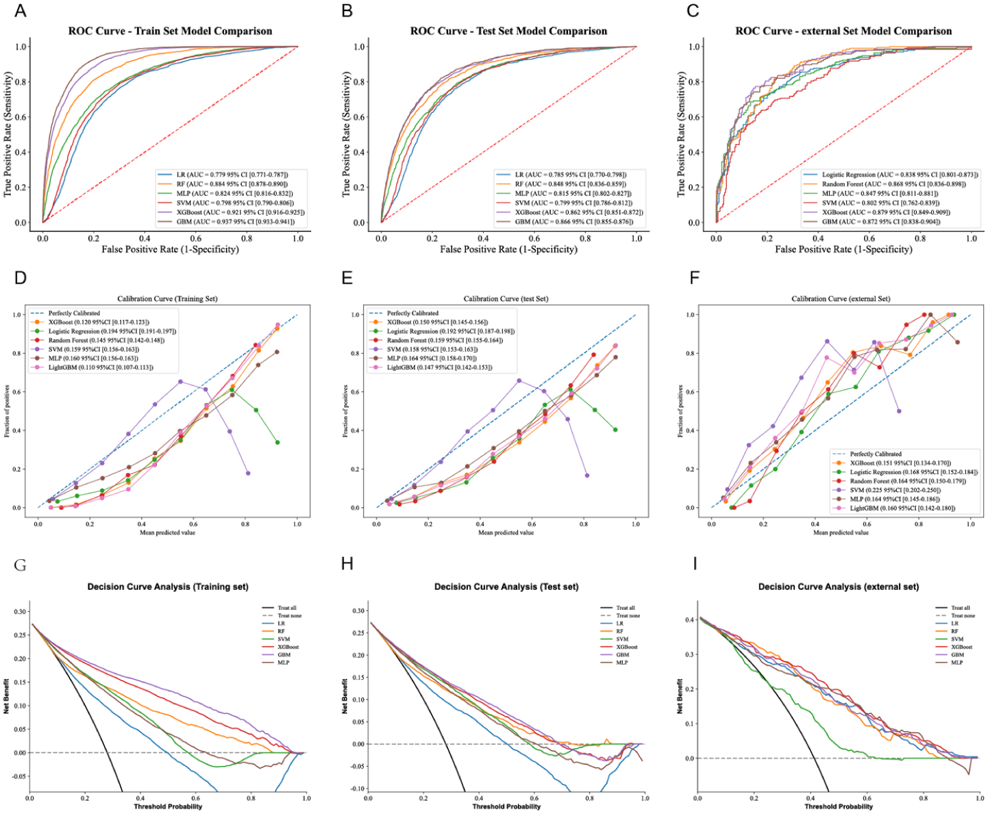
The performance and comparison of six different predictive models. (a) ROC curves for the training set, (b) ROC curves for the test set, (c) ROC curves for the validation set, (d) calibration curve for the test set, (e) calibration curve for the validation set, (f) decision curve analysis for the test set, (g) decision curve analysis for the validation set, (h) precision-recall curves for the test set, (i) precision-recall curves for the validation set.

Baseline comparison between the two cohorts revealed significant differences in age and the majority of laboratory indices, including ESR, MLR, MCH, RBC, PLR, NEUT, and MCV (all P < 0.05; Supplemental Table S3). Additional model evaluation metrics are provided in Supplemental Table S4. After a comprehensive analysis, although XGBoost, RF, SVM, LR, and MLP also showed strong predictive performance, LightGBM was considered more stable across different datasets, making it the optimal model.

AUC value advantage of the LightGBM model in clinical diagnosis

The AUC is a key metric for assessing the discriminative ability of diagnostic models or biomarkers, where a value closer to 1 indicates stronger diagnostic performance. Figure 4(a) and (b) present the ROC curves for the LightGBM model, which achieved high discriminative power in both the training set (AUC = 0.937) and the test set (AUC = 0.866). To further evaluate the model’s clinical utility, we compared its performance against four established hematologic biomarkers: ESR, NLR, MLR, and PLR. As shown in Figure 4(c; training set) and (d; test set), the AUC values for these individual biomarkers ranged from 0.552 to 0.597, which were substantially lower than those achieved by the LightGBM model. Specifically, in the test set, the AUC of the LightGBM model (0.866) significantly outperformed ESR (0.590), NLR (0.559), MLR (0.568), and PLR (0.595). Additional diagnostic metrics—including ACC, SEN, SPE, PPV, and NPV—are detailed in Supplemental Table S5. These findings demonstrate that the LightGBM model provides significantly greater precision in distinguishing AS patients from controls compared to the standalone use of traditional biomarkers, which fail to meet stringent clinical requirements.

Figure 4.

ROC curves evaluating the performance of the LightGBM model and clinical biomarkers. (a) ROC curve for the LightGBM model on the training set, (b) ROC curve for the LightGBM model on the test set, (c) comparison of ROC curves for individual clinical biomarkers on the training set: ESR (AUC = 0.597), NLR (AUC = 0.552), MLR (AUC = 0.559), and PLR (AUC = 0.589), (d) comparison of ROC curves for individual clinical biomarkers on the test set: ESR (AUC = 0.590), NLR (AUC = 0.559), MLR (AUC = 0.568), and PLR (AUC = 0.595).

Explainable machine learning model

The SHAP feature importance plot and SHAP summary plot (Figure 5) elucidate the interpretability of the LightGBM model, highlighting the 10 most influential features. These key determinants of the model’s final output predominantly encompass blood cell indices and their potential derivatives, alongside demographic characteristics. Notably, 8 out of the 10 key variables were hematologic parameters (PLT, MLR, MCH, RBC, PCT, PLR, NEUT, and MCV), underscoring their pivotal roles in the model’s predictive performance. Therefore, we further analyzed the key blood cell indices.

Figure 5.

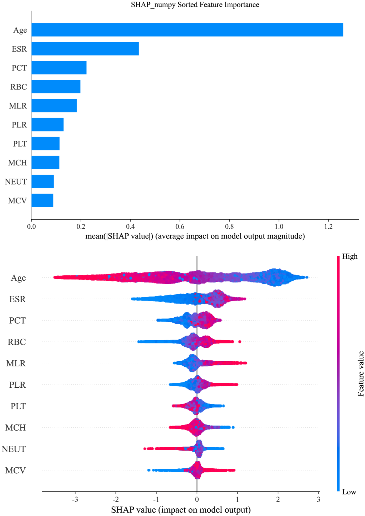
Global interpretation of the LightGBM model and feature importance. The SHAP summary plot shows key features affecting the ability of the LightGBM model to predict ankylosing spondylitis. The features are ranked on the y-axis by significance, with higher-ranked features indicating greater importance. Each dot represents a patient, with its color indicating the feature value—blue for lower values and red for higher values. The position of the dot on the x-axis (SHAP value) reflects the feature’s impact on the model’s output, indicating the likelihood of a clinical diagnosis, with higher SHAP values corresponding to a higher probability of ankylosing spondylitis.

The SHAP waterfall plots for randomly selected patients (Figure 6) illustrate that the hierarchical influence and impact direction of various parameters vary significantly across individuals, starting from a consistent baseline expected value (E[f(X)] = −0.728). For sample 1 (Figure 6(a)), the predicted value reached 0.311, a substantial increase over the expectation, predominantly driven by positive contributions from MLR = 0.581 (+0.73), ESR = 23.2 mm/h (+0.52), and MCV = 96.12 fL (+0.52), which outweighed the negative adjustment of age (68 years, −0.51). Conversely, Sample 123 (Figure 6(b)) exhibited a markedly lower prediction of −2.126, largely due to strong inhibitory effects from age (59 years, −0.8), MLR = 0.188 (−0.33), and RBC = 4.38 × 10¹²/L (−0.26). In sample 1568 (Figure 6(c)), a predicted value of 0.5 was observed, characterized by robust positive influences from MLR = 0.472 (+0.5) and ESR = 30.4 mm/h (+0.48) that were partially counteracted by MCH = 32.64 pg (−0.33) and RBC = 3.55 × 10¹²/L (−0.24). Sample 5251 (Figure 6(d)) yielded the highest prediction (0.928) among the analyzed cases, primarily attributed to the significant positive impacts of MLR = 0.667 (+0.72) and RBC = 6.22 × 10¹²/L (+0.61). Overall, the SHAP waterfall analysis identifies MLR, ESR, age, and RBC as the critical determinants of the prediction outcomes.

Figure 6.

The SHAP waterfall plot shows the predictions of a machine learning model for a specific example. Panels (a) through (d) represent samples with 1, 123, 1568, and 5251 patients, respectively. Each panel lists the top 10 clinical features contributing to the prediction: MLR, ESR, MCV, age, PCT, PLT, MCH, RBC, PLR, and NEUT. Red bars indicate positive SHAP values, representing features that increase the probability of an AS diagnosis; conversely, blue bars indicate negative SHAP values, representing features that reduce the predicted probability. The bottom value (E[f(X)] = −0.728) represents the expected (baseline) model output across the dataset, while the top value (f(X)) represents the final predicted log-odds for that specific sample.

The SHAP dependence plots in Supplemental Figure 1 illustrate the complex, nonlinear influence of clinical variables on the model output, revealing distinct biological thresholds for AS risk. Age followed a prominent unimodal trajectory, peaking at approximately 30 years and exerting a sustained positive contribution between the ages of 20 and 45 before transitioning to a negative impact (protective effect) beyond the 45-year mark. Regarding inflammatory indicators, ESR maintained significant positive SHAP values within the range of 20–80 mm/h, while the risk contributions of PLR and MLR increased progressively once their ratios exceeded 200 and 0.3, respectively. In terms of hematologic parameters, PLT counts exceeding 300 × 10⁹/L, PCT values between 0.2% and 0.4%, and RBC counts surpassing 4.8 × 10¹²/L were all associated with a higher likelihood of AS. Notably, MCH and MCV exhibited a characteristic “risk-valley” phenomenon, with their risk contributions reaching a nadir at 28–32 pg and approximately 92 fL, respectively. Conversely, NEUT maintained a relatively stable and slightly negative contribution across its clinical range. These SHAP-derived insights highlight the nonlinear drivers of AS risk, which informed the subsequent binary LR analysis to further quantify the statistical associations within these identified clinical ranges.

Synergistic effects of blood cell indices on AS

PDPs in Supplemental Figure 2 provide a detailed characterization of the synergistic interactions between key clinical variables and their collective impact on the predicted probability of AS. A prominent threshold effect was observed for ESR in Supplemental Figure 2A–C, where the predicted risk escalated sharply once ESR exceeded 20 mm/h, particularly when interacting with an MLR >0.4, a PCT >0.25%, or an RBC count >5.0 × 10¹²/L. Furthermore, interactions among other hematologic indices (Supplemental Figure 2D–F) revealed that the concurrent elevation of MLR, PCT, and RBC is associated with a progressive and synergistic increase in the predicted likelihood of the disease. Collectively, these PDP-derived findings underscore that while ESR remains a critical driver of the predicted risk, its complex interplay with indices such as MLR and RBC provides a more nuanced and multidimensional assessment of AS risk.

Association between blood cell indices and the risk of AS

The relationships between eight blood count indices and the risk of AS were evaluated using binary LR (Table 1). Results are presented as standardized ORs to allow for comparison across features with different scales. In addition, to enhance clinical interpretability, we also reported OR based on original clinical units in Supplemental Table S7.

Table 1.

Associations between blood count indices and the risk of AS.

Blood count indices	Model I		Model II
Blood count indices	OR (95% CI)	P value	OR (95% CI)	P value
Discovery cohort
PLT	1.36 (1.32–1.42)	<0.001	1.21 (1.15–1.27)	<0.001
MLR	1.26 (1.21–1.31)	<0.001	1.11 (1.01–1.21)	0.025
MCH	0.78 (0.75–0.81)	<0.001	1.01 (0.95–1.08)	0.716
RBC	1.05 (1.01–1.09)	0.007	0.96 (0.90–1.03)	0.270
PCT	1.42 (1.37–1.47)	<0.001	1.19 (1.14–1.25)	<0.001
PLR	1.37 (1.32–1.42)	<0.001	1.16 (1.10–1.24)	<0.001
NEUT	1.10 (1.06–1.14)	<0.001	0.82 (0.73–0.91)	<0.001
MCV	0.80 (0.78–0.83)	<0.001	1.02 (0.97–1.08)	0.437
External validation cohort
PLT	2.81 (2.10–3.76)	<0.001	4.07 (1.80–9.19)	<0.001
MLR	2.69 (2.02–3.57)	<0.001	2.31 (0.55–9.75)	0.255
MCH	0.58 (0.46–0.74)	<0.001	1.81 (0.88–3.75)	0.108
RBC	0.76 (0.61–0.95)	0.016	0.47 (0.22–0.97)	0.041
PCT	5.35 (3.62–7.92)	<0.001	4.81 (2.02–11.43)	<0.001
PLR	3.46 (2.40–4.97)	<0.001	3.35 (1.45–7.72)	0.005
NEUT	2.39 (1.82–3.13)	<0.001	2.03 (0.73–5.68)	0.178
MCV	0.84 (0.67–1.04)	0.109	1.98 (1.09–3.49)	0.025

Model I: Adjusted for age, sex. Model II: model I with additional adjustment for HCT, MCHC, MPV, PDW, LYMPH, LYMPH%, MONO, MONO%, BASO, BASO%, EO, EO%, RDW, NLR. Bold values indicate statistical significance (P < 0.05). CI: confidence interval; OR: odds ratio; AS: ankylosing spondylitis; NLR: neutrophil-to-lymphocyte ratio; MLR: monocyte-to-lymphocyte ratio; PLR: platelet-to-lymphocyte ratio; RBC: red blood cell; HCT: hematocrit percentage; MCV: mean corpuscular volume; MCH: mean corpuscular hemoglobin; MCHC: mean corpuscular hemoglobin concentration; RDW: red blood cell distribution width; BASO: basophil count; BASO%: basophil percentage; EO: eosinophil count; EO%: eosinophil percentage; MONO: monocyte count; MONO%: monocyte percentage; NEUT: neutrophil count; LYMPH: lymphocyte count; LYMPH%: lymphocyte percentage; PLT: platelet count; PCT: platelet crit; MPV: mean platelet volume; PDW: platelet distribution width.

In the discovery cohort (model I), all eight indicators showed significant associations with AS risk. Elevated PCT (OR: 1.42, 95% CI: 1.37–1.47, P < 0.001), PLR (OR: 1.37, 95% CI: 1.32–1.42, P < 0.001), PLT (OR: 1.36, 95% CI: 1.32–1.42, P < 0.001), MLR (OR: 1.26, 95% CI: 1.21–1.31, P < 0.001), NEUT (OR: 1.10, 95% CI: 1.06–1.14, P < 0.001), and RBC (OR: 1.05, 95% CI: 1.01–1.09, P = 0.007) were identified as risk factors. Conversely, elevated MCH (OR: 0.78, 95% CI: 0.75–0.81, P < 0.001) and MCV (OR: 0.80, 95% CI: 0.78–0.83, P < 0.001) demonstrated protective effects.

In the external validation cohort, PLT, PCT, and PLR remained robust risk factors across both models (P < 0.01). Notably, in model II of the external data, PCT showed the strongest association (OR: 4.81, 95% CI: 2.02–11.43, P < 0.001). In contrast to the discovery cohort, RBC was negatively associated with AS risk in the external cohort (model II OR: 0.47, P = 0.041), whereas MCV transitioned from a protective factor to a risk factor (model II OR: 1.98, P = 0.025). Furthermore, MLR (P = 0.255), MCH (P = 0.108), and NEUT (P = 0.178) failed to maintain statistical significance in the fully adjusted external model (Table 1).

Stratified analyses further highlighted the modulatory effects of sex and age (Supplemental Table S8). Sex-stratified analyses indicated that RBC showed opposite effects by sex, being positively associated with AS risk in males but negatively associated in females. PCT remained a consistent risk factor across both sexes. Age-stratified analyses revealed that younger individuals (<20 and 20–40 years) exhibited stronger associations for RBC and PCT, while the protective effects of MCH diminished with advancing age (Supplemental Table S9). These findings suggest that the clinical utility of these hematologic indices in predicting AS risk is significantly modified by demographic factors.

Discussion

This study developed and validated a LightGBM ML model based on routine hematologic parameters to assist in AS diagnosis. AS is a chronic inflammatory disease characterized by insidious onset and delayed radiographic manifestations. Traditional diagnostic methods rely on radiographic evidence of sacroiliitis, which typically emerges several years after disease onset, thereby contributing to delayed diagnosis.^39,40

The LightGBM model demonstrated superior diagnostic performance compared with RF, SVM, MLP, XGBoost, and LR. These findings emphasize the ability of the LightGBM model to capture complex patterns within hematologic data, though its clinical utility in AS diagnosis requires validation against imaging-based standards and in a multicenter case-control study. Another advantage of the LightGBM model is its reliance on routinely available clinical parameters. The features utilized by the model include PLT, age, MLR, MCH, RBC, ESR, PCT, PLR, NEUT, and MCV. These widely accessible and cost-effective parameters suggest potential for implementation in diverse healthcare settings.^41,42

RFE analysis identified 10 key hematologic features that maintain high diagnostic accuracy (AUC 0.866 in the test set) while significantly simplifying clinical application.⁴³ By focusing on this compact set of indices, the model provides a practical diagnostic option for clinics with limited infrastructure or EHR connectivity, balancing operational simplicity with the robust performance (AUC 0.872) confirmed in external validation.

Notably, despite the observed differences in age and certain hematologic distributions between the internal and external cohorts, the LightGBM model maintained robust performance. This stability suggests that the model is not overly sensitive to minor population shifts, further substantiating its strong generalizability and potential for deployment across different clinical settings. The model’s design suggests possible utility as an adjunct screening tool in resource-limited areas; however, its actual clinical impact on expediting the diagnostic process and referral pathways warrants further evaluation.⁴⁴

Due to their “black box” nature, ML models often encounter skepticism in the medical domain. Clinicians frequently lack insight into the decision-making mechanisms of these models, which hinders their effective integration into clinical diagnosis and treatment.^45,46 To address this limitation, this study employed the SHAP method to enhance the interpretability of the LightGBM model through waterfall plots and dependency graphs.^35,47 The SHAP waterfall plots elucidate the specific logic behind individual predictions relative to the baseline expected value (E[f(X)] = −0.728). For instance, in sample 1, the predicted risk escalated to 0.311, primarily driven by the robust positive contributions of MLR (0.581) and ESR (23.2 mm/h). Conversely, Sample 123 yielded a significantly lower prediction (−2.126), where advanced age (59 years) and a low MLR (0.188) exerted dominant inhibitory effects. Such personalized explanation paths—as further demonstrated in samples 1568 and 5251—empower clinicians to implement tailored intervention strategies based on a patient’s unique hematologic profile. SHAP dependence plots identified critical nonlinear thresholds for AS risk. Age exhibited a distinctive unimodal trajectory, peaking at approximately 30 years before transitioning to a protective effect beyond the age of 45. Notably, hematologic indices displayed complex biological windows; for instance, MCH (28–32 pg) and MCV (92 fL) exhibited a characteristic “risk-valley” phenomenon, where risk contributions reached their nadir. Furthermore, risk scores increased progressively once PLR and MLR exceeded 200 and 0.3, respectively. These findings transcend traditional linear assumptions, accurately mapping the intricate associations between hemogram parameters and AS pathology. Synergistic interactions and multidimensional risk assessment PDP analysis further revealed that AS risk is not driven by isolated parameters but rather by synergistic interactions among multiple factors. A prominent threshold effect was observed for ESR; when ESR exceeded 20 mm/h in conjunction with an elevated MLR (>0.4) or RBC count (>5.0 × 10¹²/L), the predicted probability of AS showed a precipitous, nonlinear increase. This multidimensional perspective underscores the necessity of integrating inflammatory markers with routine blood indices to achieve a more nuanced clinical evaluation.

To further bolster the clinical credibility of the SHAP-based interpretations, binary LR was employed to cross-validate the associations between hematologic indices and AS risk. The regression results demonstrated that PCT, PLT, and PLR served as robust risk factors across both the discovery. These statistical findings are in concordance with the SHAP dependency trajectories. This synergy between ML-driven interpretability and traditional statistical validation not only reinforces the biological plausibility of our model’s predictions but also facilitates clinical adoption by presenting findings through familiar metrics such as ORs and confidence intervals (CI).

The relationship between blood cell indices and the pathogenesis of AS involves multiple interrelated mechanisms.^48,49 In this study, robust associations were observed between AS risk and platelet-related indicators (PLT, PCT, and PLR), which may reflect systemic inflammation and immune dysregulation in AS patients.¹⁶ Platelet-related indices are particularly relevant in AS-associated inflammation. Elevated PLT, PCT, and PLR were significantly correlated with increased AS risk, possibly because of the release of proinflammatory cytokines (such as IL-1β and TNF-α) by platelets, activation of monocytes and neutrophils, and exacerbation of inflammatory responses.⁴⁹ These findings suggest that abnormal platelet function may represent a key driver and therapeutic target in the pathogenesis of AS.

In summary, the observed associations between blood cell indices and AS risk provide important clues for understanding its pathogenesis. Notably, while these indices—such as PLT, PCT, and PLR—show individual associations with AS, they are inherently biologically and mathematically coupled. Although our analysis confirmed that the VIF for these variables was below 10, their physiological interdependence should be explicitly acknowledged. Therefore, the interpretation of these findings should consider these indices as a collective reflection of the platelet and inflammatory profile rather than as entirely independent biological drivers. Nevertheless, the underlying biological mechanisms require further investigation in future studies.

While our hematology-based LightGBM model demonstrated robust discriminatory performance, several limitations warrant consideration. First, data constraints precluded the inclusion of conventional biomarkers such as HLA-B27 and CRP, which may limit the model’s practical utility in some clinical settings. Second, although externally validated, our cohort was restricted to two institutions within a single region, potentially limiting generalizability across diverse populations. Third, as a retrospective study, a formal prestudy power analysis was not performed; however, the inclusion of all 17,504 eligible participants available during the study period provided substantial statistical power for model development. Most importantly, our reliance on the revised New York criteria—which requires definitive radiographic sacroiliitis—inherently excludes patients with nonradiographic axial spondyloarthritis or those in very early stages before structural damage appears on X-ray. Consequently, while the model is effective for identifying established AS, its clinical utility as a standalone “early detection” tool remains to be validated in preradiographic cohorts. Future studies incorporating MRI-detected bone marrow edema or early inflammatory markers are essential to confirm the model’s sensitivity for early-stage detection. Finally, the underlying mechanistic roles of the identified blood indices in AS pathogenesis require further substantiation through experimental studies.

Conclusions

This study developed and internally validated a diagnostic model for AS, with its performance further assessed through external validation. Interpretable ML techniques were employed to elucidate significant associations between key hematologic parameters and AS, and the final model demonstrated reliable diagnostic performance. In addition, this population-based retrospective case-control study explored the relationships between blood cell indices and AS, providing insights into the molecular mechanisms underlying disease pathogenesis.

Supplemental Material

sj-doc-1-smo-10.1177_20503121261424338 – Supplemental material for Associations of blood cell indices with the risk of ankylosing spondylitis: A retrospective case-control and machine learning modeling study

Supplemental material, sj-doc-1-smo-10.1177_20503121261424338 for Associations of blood cell indices with the risk of ankylosing spondylitis: A retrospective case-control and machine learning modeling study by Rongqing He, Kechang He, Xiaopeng Qin, Jie Ma, Zhuo Chen, Boli Qin, Jiang Xue, Tianyou Chen, Jiarui Chen, Xinli Zhan and Chong Liu in SAGE Open Medicine

Supplemental Material

sj-docx-2-smo-10.1177_20503121261424338 – Supplemental material for Associations of blood cell indices with the risk of ankylosing spondylitis: A retrospective case-control and machine learning modeling study

Supplemental material, sj-docx-2-smo-10.1177_20503121261424338 for Associations of blood cell indices with the risk of ankylosing spondylitis: A retrospective case-control and machine learning modeling study by Rongqing He, Kechang He, Xiaopeng Qin, Jie Ma, Zhuo Chen, Boli Qin, Jiang Xue, Tianyou Chen, Jiarui Chen, Xinli Zhan and Chong Liu in SAGE Open Medicine

Supplemental Material

sj-docx-3-smo-10.1177_20503121261424338 – Supplemental material for Associations of blood cell indices with the risk of ankylosing spondylitis: A retrospective case-control and machine learning modeling study

Supplemental material, sj-docx-3-smo-10.1177_20503121261424338 for Associations of blood cell indices with the risk of ankylosing spondylitis: A retrospective case-control and machine learning modeling study by Rongqing He, Kechang He, Xiaopeng Qin, Jie Ma, Zhuo Chen, Boli Qin, Jiang Xue, Tianyou Chen, Jiarui Chen, Xinli Zhan and Chong Liu in SAGE Open Medicine

Footnotes

Acknowledgements

We are very grateful to Prof. Chong Liu and Prof. Xinli Zhan (Spine and Osteopathy Ward, The First Affiliated Hospital of Guangxi Medical University), Prof. Jie Ma (Surgical Ward, The Fourth People’s Hospital of Nanning, Nanning, Guangxi, China) for their support in all stages of this study.

ORCID iD

Chong Liu

Author contributions

Rongqing He, Kechang He, and Jie Ma participated in the conceptualization and methodology design of the study. Boli Qin, Tianyou Chen, and Jiarui Chen were in charge of data curation and investigation. Zhuo Chen, Jiang Xue, and Xiaopeng Qin analyzed and visualized the data. Chong Liu and Xinli Zhan: Writing-Reviewing and Editing. All authors contributed to the article and approved the submitted version.

Funding

The authors disclosed receipt of the following financial support for the research, authorship, and/or publication of this article: (1) The National Natural Science Foundation of China (Grant number: NSFC82360422); (2) Joint Project on Regional High-Incidence Diseases Research of Guangxi Natural Science Foundation (Grant number: 2024GXNSFAA010073); (3) Guangxi Young and Middle aged Teacher’s Basic Ability Promoting Project (Grant number: 2023KY0115); (4) The “Medical Excellence Award” Funded by the Creative Research Development Grant from the First Affiliated Hospital of Guangxi Medical University; (5) Clinical Research Climbing Plan Project of the First Affiliated Hospital of Guangxi Medical University in 2023 (Grant number: YYZS2023008); (6) Innovation Project of Guangxi Graduate Education (Grant number: JGY2024094); (7) Guangxi Zhuang Autonomous Region “Four New” Research and Practice Project (Grant number: SX202319); (8) Guangxi Medical and Health Appropriate Technology Development and Promotion Project (Grant number: S2024017); (9) First-class discipline innovation-driven talent program of Guangxi Medical University. Funding bodies had not participated in the design of the study, collection, interpretation, and analysis of the data, or in writing the manuscript.

Declaration of conflicting interests

The authors declared no potential conflicts of interest with respect to the research, authorship, and/or publication of this article.

Data availability statement

The original contributions presented in the study are included in the article/Supplemental Material; further inquiries can be directed to the corresponding authors.

Generative AI and AI-assisted technologies in the writing process

No generative AI or AI-assisted technologies were used in the writing process of this manuscript. All content was authored independently by the researchers.

Supplemental material

Supplemental material for this article is available online.

References

Paluch-Oles

Magrys

Koziol-Montewka

, et al. Identification of latent tuberculosis infection in rheumatic patients under consideration for treatment with anti-TNF-alpha agents. Arch Med Sci 2013; 9(1): 112–117.

Solmaz

Bakirci

Jibri

, et al. Psoriasis is an independent risk factor for entheseal damage in axial spondyloarthritis. Semin Arthritis Rheum 2020; 50(1): 42–47.

Chen

JY.

Ankylosing spondylitis: Chinese perspective, clinical phenotypes, and associated extra-articular systemic features. Curr Rheumatol Rep 2013; 15(8): 344.

van der Heijde

Cheng-Chung Wei

Dougados

, et al. Ixekizumab, an interleukin-17A antagonist in the treatment of ankylosing spondylitis or radiographic axial spondyloarthritis in patients previously untreated with biological disease-modifying anti-rheumatic drugs (COAST-V): 16 week results of a phase 3 randomised, double-blind, active-controlled and placebo-controlled trial. Lancet 2018; 392(10163): 2441–2451.

Ash

Marzo-Ortega

Ankylosing spondylitis–the changing role of imaging. Skelet Radiol 2012; 41: 1031–1034.

Xiao

Huang

, et al. Serum metabolomics signatures associated with ankylosing spondylitis and TNF inhibitor therapy. Front Immunol 2021; 12: 630791.

Fallahi

Jamshidi

AR.

Diagnostic delay in ankylosing spondylitis: related factors and prognostic outcomes. Arch Rheumatol 2016; 31(1): 24–30.

Swanson

Zhang

, et al. From patterns to patients: Advances in clinical machine learning for cancer diagnosis, prognosis, and treatment. Cell 2023; 186(8): 1772–1791.

Sariyildiz

Benlidayi

Turk

, et al. Evaluation of the relationship between blood cell markers and inflammation, disease activity, and general health status in ankylosing spondylitis. Rev Assoc Med Bras (1992) 2023; 69(10): e20230722.

10.

Zhuang

Huang

Liang

Clinical significance of the monocyte:lymphocyte ratio for ankylosing spondylitis patients with thoracolumbar kyphotic deformities. J Int Med Res 2020; 48(1): 300060519893167.

11.

Zhou

Chen

, et al. Platelet indices in patients with chronic inflammatory arthritis: a systematic review and meta-analysis. Platelets 2020; 31(7): 834–844.

12.

Inci

Effect of ozone therapy on neutrophil/lymphocyte, platelet/lymphocyte ratios, and disease activity in ankylosing spondylitis: a self-controlled randomized study. Med Gas Res 2023; 13(2): 53–58.

13.

Liang

Chen

, et al. Platelet-to-lymphocyte ratio as an independent factor was associated with the severity of ankylosing spondylitis. Front Immunol 2021; 12: 760214.

14.

Zhang

KF.

What’s the relative risk? A method of correcting the odds ratio in cohort studies of common outcomes. JAMA 1998; 280(19): 1690–1691.

15.

Von Elm

Altman

Egger

, et al. The Strengthening the Reporting of Observational Studies in Epidemiology (STROBE) statement: guidelines for reporting observational studies. Lancet 2007; 370(9596): 1453–1457.

16.

Haroon

Paterson

, et al. Patients with ankylosing spondylitis have increased cardiovascular and cerebrovascular mortality: a population-based study. Ann Intern Med 2015; 163(6): 409–416.

17.

Batista

Monard

MC.

An analysis of four missing data treatment methods for supervised learning. Appl Artif Intell 2003; 17(5–6): 519–533.

18.

Mining

WID

. Data mining: concepts and techniques. Morgan Kaufinann, 2006.

19.

Shanker

Hung

MS.

Effect of data standardization on neural network training. Omega 1996; 24(4): 385–397.

20.

Garcia

EA.

Learning from imbalanced data. IEEE Trans Knowl Data Eng 2009; 21(9): 1263–1284.

21.

Han

Gondro

Reid

, et al. Heuristic hyperparameter optimization of deep learning models for genomic prediction. G3 (Bethesda) 2021; 11(7): jkab032.

22.

Glenn

WB.

Verification of forecasts expressed in terms of probability. Mon Weather Rev 1950; 78(1): 1–3.

23.

Rijsbergen

CV.

Information retrieval. Butterworth-Heinemann, 1979.

24.

Yesilyaprak

Kumar

Agrawal

, et al. Predicting long-term clinical outcomes of patients with recurrent pericarditis. J Am Coll Cardiol 2024; 84(13): 1193–1204.

25.

Lundberg

A unified approach to interpreting model predictions. arXiv Preprint 2017; 2017: arXiv:170507874.

26.

Scott

Su-In

A unified approach to interpreting model predictions. Adv Neural Inf Process Syst 2017; 30: 4765–4774.

27.

Kraev

Koseoglu

Traverso

, et al. Shap-select: lightweight feature selection using SHAP values and regression. arXiv Preprint 2024; 2024: arXiv:241006815.

28.

Mihirette

Tan

(eds.) SHAP algorithm for healthcare data classification. In: Bringas

Pérez García

Martínez de Pisón

, et al. (eds) Hybrid Artificial Intelligence Systems. HAIS 2022, Salamanca, Spain, 5-7 September 2022. Springer, Cham.

29.

Zhang

Variable selection with stepwise and best subset approaches. Ann Transl Med 2016; 4(7): 136.

30.

Lazzarini

Bacardit

RGIFE: a ranked guided iterative feature elimination heuristic for the identification of biomarkers. BMC Bioinformatics 2017; 18(1): 322.

31.

Meiseles

Rokach

Iterative Feature eXclusion (IFX): mitigating feature starvation in gradient boosted decision trees. Knowl Based Syst 2024; 289: 111546.

32.

Vellido

The importance of interpretability and visualization in machine learning for applications in medicine and health care. Neural Comput Appl 2020; 32(24): 18069–18083.

33.

Apley

Zhu

Visualizing the effects of predictor variables in black box supervised learning models. J R Stat Soc Ser B Stat Methodol 2020; 82(4): 1059–1086.

34.

Nohara

Matsumoto

Soejima

, et al. Explanation of machine learning models using shapley additive explanation and application for real data in hospital. Comput Methods Programs Biomed 2022; 214: 106584.

35.

Ponce-Bobadilla

Schmitt

Maier

, et al. Practical guide to SHAP analysis: Explaining supervised machine learning model predictions in drug development. Clin Transl Sci 2024; 17(11): e70056.

36.

Zhang

, et al. Machine learning combined with the PMF model reveal the synergistic effects of sources and meteorological factors on PM(2.5) pollution. Environ Res 2022; 212(Pt B): 113322.

37.

Chang

Chu

Chen

, et al. The comparison and interpretation of machine-learning models in post-stroke functional outcome prediction. Diagnostics (Basel) 2021; 11(10): 1784.

38.

Park

Lee

Kim

, et al. Interpretation of ensemble learning to predict water quality using explainable artificial intelligence. Sci Total Environ 2022; 832: 155070.

39.

Navarro-Compan

An update on diagnosis and classification of axial spondyloarthritis. Curr Rheumatol Rep 2019; 21(8): 39.

40.

Song

Sieper

Rudwaleit

Diagnosing early ankylosing spondylitis. Curr Rheumatol Rep 2007; 9(5): 367–374.

41.

Seo

Lee

YJ.

Usefulness of complete blood count (CBC) to assess cardiovascular and metabolic diseases in clinical settings: a comprehensive literature review. Biomedicines 2022; 10(11): 2697.

42.

Tefferi

Hanson

Inwards

DJ.

How to interpret and pursue an abnormal complete blood cell count in adults. Mayo Clin Proc 2005; 80(7): 923–936.

43.

Wang

Huang

, et al. Construction of machine learning diagnostic models for cardiovascular pan-disease based on blood routine and biochemical detection data. Cardiovasc Diabetol 2024; 23(1): 351.

44.

Shah

Kendall

Khozin

, et al. Artificial intelligence and machine learning in clinical development: a translational perspective. NPJ Digit Med 2019; 2: 69.

45.

Petch

Nelson

Opening the black box: the promise and limitations of explainable machine learning in cardiology. Can J Cardiol 2022; 38(2): 204–213.

46.

Rudin

Stop explaining black box machine learning models for high stakes decisions and use interpretable models instead. Nat Mach Intell 2019; 1(5): 206–215.

47.

Orlenko

Moore

JH.

A comparison of methods for interpreting random forest models of genetic association in the presence of non-additive interactions. BioData Min 2021; 14(1): 9.

48.

Rezaiemanesh

Abdolmaleki

Abdolmohammadi

, et al. Immune cells involved in the pathogenesis of ankylosing spondylitis. Biomed Pharmacother 2018; 100: 198–204.

49.

Gasparyan

Ayvazyan

Mukanova

, et al. The platelet-to-lymphocyte ratio as an inflammatory marker in rheumatic diseases. Ann Lab Med 2019; 39(4): 345–357.

Supplementary Material

Please find the following supplemental material available below.

For Open Access articles published under a Creative Commons License, all supplemental material carries the same license as the article it is associated with.

For non-Open Access articles published, all supplemental material carries a non-exclusive license, and permission requests for re-use of supplemental material or any part of supplemental material shall be sent directly to the copyright owner as specified in the copyright notice associated with the article.

0.00 MB

0.07 MB

1.03 MB

0.07 MB