Explainable machine learning for early diagnosis of esophageal cancer: A feature-enriched Light Gradient Boosting Machine framework with Shapley Additive Explanations and Local Interpretable Model-Agnostic Explanations interpretations

Abstract

Objective

Esophageal cancer is among the most rapidly spreading malignancies worldwide. Early detection of esophageal cancer is critical for disease prevention and for improving overall population health. Most studies have used statistical methodologies to assess the esophageal cancer risk, and only a few studies have used prediction models.

Methods

The esophageal cancer dataset, comprising 3985 patient records with 85 demographic, pathological, and follow-up features, was obtained from Kaggle. A comprehensive data-engineering pipeline was implemented, including the removal of null and low-variance features, elimination of identifier variables to prevent data leakage, mode-based imputation, label encoding, and data standardization. Feature relevance was assessed using Mutual Information, and the top 31 clinically meaningful features were retained for model development. Six machine learning classifiers—Support Vector Machine, Gaussian Naïve Bayes, k-nearest neighbors, AdaBoost, Multilayer Perceptron, and LightGBM (Gradient Boosting Machine)—were trained and evaluated. A stratified 10-fold cross-validation was applied to maintain class balance, and GridSearchCV was used for hyperparameter optimization. Model interpretability was assessed using Shapley Additive Explanations (SHAP) for global and local feature attribution and Local Interpretable Model-Agnostic Explanations (LIME) for instance-level explanations. Furthermore, the top features identified by SHAP and LIME were used to retrain the LightGBM model to evaluate performance under reduced dimensionality.

Results

Among all evaluated classifiers, LightGBM exhibited the highest and most stable performance, achieving an accuracy of 99.87% prior to hyperparameter tuning and 99.74% following stratified cross-validated tuning, with near-perfect precision, recall, F1-score, and area under the curve values. Explainability analyses indicated that clinically relevant variables, including tumor staging, smoking-related factors, and follow-up indicators, played a significant role in model predictions. The SHAP-selected top-20 feature model maintained high predictive performance (99.76%), demonstrating that the classifier remained robust despite dimensionality reduction.

Conclusions

The proposed LightGBM-based model demonstrates exceptional predictive accuracy and strong interpretability, suggesting its potential utility for the early detection of esophageal cancer using machine learning approaches.

Introduction

Esophageal cancer (EC) refers to aggressive malignant neoplasms of the upper digestive tract that originate from the esophageal epithelium and comprise two major histological subtypes: squamous cell carcinoma and adenocarcinoma (AC). ¹ Nearly six million new cases of EC are reported globally each year. ² On average, men are three to four times more likely than women to develop EC worldwide. ³ In Asian countries such as China and Japan, SCC is the predominant histological type. In contrast, risk factors play a significant role in the high prevalence of AC in the United States and Europe. ⁴ EC is the eighth most common cancer worldwide and the sixth leading cause of cancer-related mortality. Moreover, the 5-year survival rate remains below 25%, ⁵ indicating a poor prognosis.

EC has multiple causes, most of which are related to chronic irritation of the esophagus.^6,7 One common factor is gastroesophageal reflux disease, in which stomach acid flows back into the esophagus, damaging its lining and potentially leading to Barrett’s esophagus, a condition that increases cancer risk. Smoking and tobacco use also damage the esophagus, particularly when combined with heavy alcohol consumption, which further irritates the tissue. Obesity is a risk factor because it can exacerbate acid reflux. Frequent consumption of very hot beverages may cause esophageal damage over time. A diet low in fruits and vegetables can increase susceptibility, as it limits the intake of nutrients that help protect the esophagus. Finally, achalasia can lead to long-term irritation and elevate cancer risk. The risk factors for EC are summarized in Figure 1.

Figure 1.

Esophageal cancer risk factors.

Globally, EC incidence is increasing, largely influenced by lifestyle factors such as smoking. ⁸ By 2030, the incidence is expected to continue rising worldwide. ⁹ In the United States, there are 17,300 new cases and 15,840 EC-related deaths reported annually. ¹⁰ Regions with the highest EC prevalence include northern and central China, central Asia, and northern Iran. ¹¹ In Iran, the age-standardized rate of EC is almost 7 per 100,000 population, and its prevalence has increased over the past decade, particularly among men. ¹² The highest incidence and mortality rates are observed in northern Iran, especially in Golestan province. ¹³

EC presents with several symptoms. ¹⁴ Difficulty swallowing is a common early sign, initially affecting the intake of solid foods and subsequently the intake of liquids. Unexplained weight loss often occurs due to reduced food intake. Pain during swallowing may manifest as a burning or sharp sensation. Chest discomfort can also occur. Some patients experience hoarseness or a persistent cough, and regurgitation of food may occur. Fatigue and weakness are common, reflecting inadequate nutritional intake. Early diagnosis of EC is crucial for improving the effectiveness of curative treatment. ¹⁵ Moreover, prompt detection can increase survival rates among EC patients. ¹⁶ The poor prognosis and rising prevalence of EC underscore the need for enhanced diagnostic and predictive strategies, supported by adequate screening procedures, to achieve preventive objectives.^17,18

Early detection of EC is critical to improving the 5-year survival rate and decreasing the death rate, as the condition is aggressive and often asymptomatic, leading to a poor prognosis.¹⁹ To achieve this goal, several researchers have developed modern technologies that use artificial intelligence (AI) for early EC diagnosis, thereby improving prognosis and ultimately increasing the patient survival rate.²⁰

Machine learning (ML) can analyze complex medical data and identify hidden relationships between patient features and cancer risk. It employs feature selection, classification, and pattern recognition to detect early signs of EC that traditional methods may miss. These data-driven techniques can make diagnosis faster, more accurate, and more cost-effective.

Therefore, ML has the potential to significantly reduce the death rate. Several types of ML methods are used to detect EC, including Support Vector Machine (SVM), Gaussian Naive Bayes (Gaussian NB), k-nearest neighbors (KNN), AdaBoost Classifier, LightGBM Classifier, and Multilayer Perceptron (MLP). First, an efficient pipeline for data preprocessing was created, incorporating data normalization, null value removal, label encoding, and missing value imputation. This pipeline enhances the ML model’s understanding of the training dataset’s features and patterns. Next, we extracted the key features for operation through feature selection.

The primary contributions of this study are as follows:

LightGBM achieved 99.74% accuracy, with precision, recall, and F1-score all above 0.99, ensuring robust early prediction of EC.

We implemented a robust preprocessing pipeline, including null value removal, low-variance filtering, imputation, encoding, and scaling. Additionally, Mutual Information (MI) was used to select clinically relevant features.

All models were optimized through systematic hyperparameter tuning and 10-fold cross-validation, ensuring stability and generalization. Six ML algorithms (SVM, Gaussian NB, KNN, AdaBoost, MLP, and LightGBM) were compared under a unified evaluation protocol, with LightGBM emerging as the best performer.

We applied SHAP (global) and Local Interpretable Model-Agnostic Explanations (LIME) (local) to enhance transparency, enabling clinical trust and bias detection. Using the top 20 features identified by SHAP and LIME, LightGBM was retrained and achieved nearly identical accuracy (SHAP: 99.76%, LIME: 99.62%) while improving efficiency and interpretability.

SHAP and LIME were compared for global and local explanations, revealing consistent key features and enabling compact models with minimal accuracy loss.

The remainder of this study is organized into four sections. Section 2 provides a concise overview of related research. Section 3 details the materials and methods used in this study for evaluating EC. Section 4 presents the results and analysis of the proposed model. Finally, Section 5 provides the study’s conclusion.

Related literature

By more effectively identifying tumor lesions in endoscopic images, Tsai et al. employed hyperspectral imaging combined with a deep learning (DL) technique for early detection of EC. According to their research, segmentation accuracy for EC images ranged from 88% to 91%.²¹ Another technological approach for early EC diagnosis was semantic segmentation, which utilized the encoder–decoder architecture of artificial neural networks. This technique used image data, including narrow-band and white-light types, to train a U-net and ResNet combination. The results of this study showed that the algorithm’s approximate accuracy was 85% for narrow-band images and 82% for white-light images.²² In a separate study, researchers used 1780 EC images with a combination of band-selective technology and hyperspectral imaging with color reproduction. They found that their early detection approach achieved reasonable diagnostic performance, with an average precision of 80%–85%.²³

Currently, prediction models are used to estimate the risk of various illnesses for screening purposes, enabling preventive strategies and improving quality of life for high-risk populations.^24,25 Several studies have employed risk prediction models based on statistical regression analysis to stratify high-risk groups for EC as a preventive measure. To identify the EC high-risk category, Chen et al. developed a risk prediction model using logistic regression. Risk factors incorporated into the model included age, sex, smoking status, concerning symptoms such as back pain, dietary variables, and a family history of upper gastrointestinal malignancies. The logistic regression–based model achieved an area under the receiver operator characteristic (ROC) curve (AU-ROC) of 0.81 for EC risk prediction.²⁶ Wang et al. developed a risk prediction model for EC using competing risk regression, incorporating indicators such as smoking, alcohol use, body mass index, physical activity, and demographic characteristics. The model achieved AU-ROCs of 0.76 and 0.70 for internal and external validations, respectively.²⁷ Etemadi et al. employed multivariate logistic regression to develop a risk prediction model for EC based on regional risk factors, including water source, tea temperature, dental health, opium consumption, and demographic features. Their model identified the EC high-risk group with an AU-ROC of 0.77.²⁸

Although statistical techniques are important for understanding relationships between variables, their reliability decreases for prediction as data volume increases. ML methodologies are useful for developing high-accuracy prediction models, particularly when handling large datasets. Furthermore, ML approaches outperform statistical predictive methods in terms of predictive capability, especially given the large data volumes and diverse data types encountered in the medical field, including image data.^29,30

By improving the use of digital data, such as electronic health records, across various medical sectors, ML, a branch of AI, has gained prominence.³¹ DL, a subfield of ML, performs well with unstructured and high-volume data types, whereas ML techniques typically use structured and tabular data.^32,33 Through retrospective and longitudinal data, ML has become increasingly popular in clinical prediction tasks.³⁴ It has been applied to predict numerous clinical conditions more accurately, including drug discovery,³⁵ geriatric status assessment,³⁶ cardiac diseases,³⁷ coronavirus disease 2019 (COVID-19),³⁸ and cancer.³⁹ Several studies worldwide have explored the use of ML for EC, including prognosis prediction, medication dosing, survival rates, and treatment-related issues. However, stratifying the EC high-risk group requires the development of an effective risk prediction model.⁴⁰ To date, most previous research has focused on creating EC prediction models using statistical techniques and risk factors, with relatively less attention given to ML-based approaches.

Materials and methods

This section discusses the procedures and materials used in this study. The process of the proposed method for identifying EC is illustrated in Figure 2. The first step involves preprocessing the dataset. Dataset preparation strategies and the ML algorithms used for diagnosis are described and analyzed. The initial step of this study was to examine the EC dataset, with several analyses conducted using six ML algorithms: SVM, Gaussian NB, KNN, AdaBoost Classifier, LightGBM Classifier, and MLP.

Figure 2.

Overview of the proposed system.

To ensure that each model was evaluated under consistent and reproducible conditions, all algorithms were trained on the same preprocessed dataset and assessed using a unified evaluation pipeline. Additionally, stratified K-fold cross-validation (K = 10) was applied across all classifiers to preserve class distribution within each fold and obtain more reliable performance estimates, particularly given the dataset’s moderate class imbalance.

In this study, a series of data preparation techniques—including null value removal, low-variability feature removal, missing value imputation, data standardization, and label encoding—were performed to ensure data quality and consistency before analysis. These preprocessing steps reduced noise, eliminated redundant or uninformative attributes, and enhanced the model’s ability to learn meaningful patterns from the data. Subsequently, MI was used to assess feature relevance to the target variable. MI scoring enabled the selection of the most informative clinical and pathological attributes, improving computational efficiency while preserving predictive power.

The data were then split into training and testing sets, with 80% allocated for training and 20% for testing, and input into the ML models. To prevent potential data leakage, all identifier- and timestamp-related columns were excluded. As the dataset lacks sequential records, temporal splitting was not required. Random shuffling was applied before splitting to ensure unbiased separation. Furthermore, to enhance model robustness, hyperparameter tuning was performed using GridSearchCV for all classifiers. This systematic search over parameter combinations helped identify the optimal configuration for each algorithm.

The final step is model assessment, which involves evaluating the performance of each ML model using various metrics, including accuracy, confusion matrix, precision, recall, and F1-score. Additionally, the AU-ROC was used to assess how effectively each model distinguishes between positive and negative cases. Subsequently, model explainability analysis was performed to identify the key factors influencing the prediction of specific classes. Feature values contributing to these outcomes were highlighted. SHAP and LIME were used to explain the model predictions.

To achieve both global and local interpretability, SHAP was used to compute feature importance across the entire model, while LIME provided instance-level explanations for individual predictions. Together, these complementary explainability tools ensured clinical transparency and helped verify that the model’s decisions aligned with known medical risk factors. The overall workflow—from preprocessing and feature selection to model training, hyperparameter optimization, evaluation, and explainability—forms a comprehensive and reproducible pipeline for early EC detection. Finally, the procedure for understanding the prediction for a single instance is described in Algorithm 1.

Dataset description

The EC dataset, comprising 3985 cases and 85 features, was acquired from Kaggle.⁴¹ It includes a mix of categorical, numerical, and clinical features. The dataset contains 55 categorical, 23 float-based numerical, and 7 integer-based numerical features. It primarily contains demographic information, clinical diagnoses, tumor stages, pathology results, and treatment histories of patients diagnosed with EC. A general overview of the dataset is provided in Table 1.

Table 1.

General overview of the dataset.

Dataset property	Description
Dataset characteristics	Multivariate
Attribute characteristics	Real
The number of features	85
Number of instances	3985
Number of features with integer-based numeric values	7
Number of features with float-based numeric values	23
Number of categorical features	55
Target column name	person_neoplasm_cancer_status
Instances are classified as	Cancer/not cancer
Number of classes defined as cancer	2570
Number of classes defined as not cancer	1415
Data source	Kaggle

Dataset preprocessing

Data preprocessing is necessary to achieve the highest level of accuracy before feeding these datasets into ML models. Preprocessing methods help address unwanted noise, missing values, outliers, label encoding, and other issues. After the data has been cleaned, ML models are applied to it.

Initially, columns containing only null values were removed to reduce duplicate features, as they provided no meaningful information. Next, specific identification columns, including patient-related properties such as “s/n,” “patient_barcode,” “patient_id,” and “bcr_patient_uuid,” were eliminated to avoid potential data leakage and ensure privacy. Subsequently, features with limited variability, identified as those carrying only a single unique value, were deleted, as they do not contribute significant differences to the dataset. The low-variability columns removed were “informed_consent_verified,” “history_of_neoadjuvant_treatment,” “project,” “primary_pathology_tumor_tissue_site,” and “primary_pathology_days_to_initial_pathologic_diagnosis.” To manage missing values, categorical and numerical features were imputed using the mode (most frequent value) to preserve data integrity without introducing biases.

To handle categorical variables, we applied label encoding using Label Encoder. We iterated through all columns with object data types and transformed their categorical values into numerical representations. This step was essential to ensure that the ML model could effectively process the data. Then, the Standard Scaler technique was used to standardize the dataset values, and the standardized data were used to train ML models.

Feature selection

It is essential to choose the most significant features⁴² before applying the ML technique. In this study, we employed the MI scoring method to determine the significance of each attribute and extract the most important ones.

MI was applied to measure the relevance of features to the target variable, selecting the top 60 features based on descending scores. Features with MI values greater than 0.05 were retained, ensuring optimal feature selection for predictive modeling.

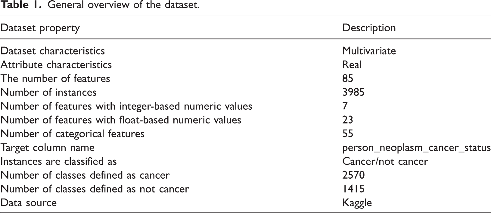
The MI scores of the selected features are displayed in Table 2. MI calculates the contribution of each feature to the prediction of the target variable. A feature associated with a higher MI score is more important for prediction. The three most important features are days_to_death (0.292), stage_event_tnm_categories (0.312), and days_to_last_followup (0.335). These features are essential for evaluating cancer progression and patient survival. Although features with MI scores above 0.05 were primarily retained, a few features with slightly lower scores (for example, primary_pathology_columnar_metaplasia_present = 0.049) were included because of their potential clinical relevance and interpretability. This approach ensured that meaningful predictors were not excluded solely due to marginal score differences.

Table 2.

Selected feature with MI score.

Features	MI score
days_to_last_followup	0.335476
stage_event_tnm_categories	0.311948
days_to_death	0.291648
tissue_source_site	0.26336
city_of_procurement	0.25873
days_to_birth	0.222679
state_province_of_procurement	0.212354
day_of_form_completion	0.193602
number_pack_years_smoked	0.191641
primary_pathology_lymph_node_examined_count	0.177043
country_of_procurement	0.165628
stopped_smoking_year	0.1567
primary_pathology_age_at_initial_pathologic_diagnosis	0.150836
has_follow_ups_information	0.138718
vital_status	0.133481
age_began_smoking_in_years	0.104188
primary_pathology_number_of_lymphnodes_positive_by_he	0.092797
tissue_prospective_collection_indicator	0.084487
primary_pathology_year_of_initial_pathologic_diagnosis	0.084128
has_new_tumor_events_information	0.081381
month_of_form_completion	0.081048
tissue_retrospective_collection_indicator	0.075784
stage_event_pathologic_stage	0.074315
year_of_form_completion	0.07232
stage_event_system_version	0.067827
stage_event_clinical_stage	0.065663
weight	0.061717
primary_pathology_planned_surgery_status	0.051403
barretts_esophagus	0.051194
primary_pathology_residual_tumor	0.050408
primary_pathology_columnar_metaplasia_present	0.050001

MI: Mutual Information.

It is important to note that these features originate from the baseline clinical registry information rather than from future outcome data. They are commonly recorded alongside diagnostic and demographic variables in retrospective datasets. Therefore, their inclusion does not introduce target leakage. In this study, these features were retained primarily to explore their statistical associations and contributions to model interpretability (via SHAP and LIME), rather than for real-time clinical prediction or screening purposes.

Other features that help predict outcomes include weight, smoking history, and age at diagnosis. Data related to pathology, such as surgical plans, tumor staging, and lymph node examination, help determine the extent of cancer and the most appropriate course of treatment. The bar chart (Figure 3) illustrates feature importance based on MI scores in the EC dataset.

Figure 3.

Feature importance based on MI score. MI: Mutual Information.

Correlation matrix

A correlation matrix describes the relationships between the parameters in a dataset. Figure 4 shows a correlation matrix heatmap, representing the correlation coefficients between different variables. The heatmap uses a color gradient ranging from blue to red, where blue indicates negative correlations and red indicates positive correlations. Some features, such as “primary_pathology_year_of_initial_pathologic_diagnosis” and “primary_pathology_age_at_initial_pathologic_diagnosis,” exhibit strong positive correlations. In contrast, other variables show weak or no correlation. This heatmap provides an efficient method to examine patterns in the dataset and identify potential predictive features.

Figure 4.

Correlation matrix heatmap.

ML models

Data mining techniques were used to generate classification templates to produce unique and interpretable patterns.⁴³ Both supervised and unsupervised learning techniques, applied in clinical and medical diagnostics for regression and classification, require the development of models based on historical data. The classification methods described in this section were applied in this study.

SVM

SVMs are supervised learning models used for classification that analyze data and identify patterns in ML. A fundamental SVM is a nonprobabilistic binary linear classifier that predicts which of the two classes will produce the output for each input.⁴⁴ Using a set of training examples labeled as belonging to one of the two categories, the SVM training approach builds a model that assigns new instances to one of these categories. By using the kernel technique, which involves implicitly converting inputs into high-dimensional feature spaces, SVMs can perform nonlinear classification in addition to linear classification.

Mathematically, an SVM can be described as follows. The training data for the two classes are stacked into a p × q matrix X. Here, p represents the number of observations and q represents the number of variables. x_i represents the i^th row of X. If each x_i belongs to class +1 or −1, this is indicated by another diagonal p × p matrix Y with −1 and +1. The main challenge in SVM is to separate the collection of training vectors into two distinct groups using a hyperplane.

$$D=\left\{\right(x1,y1),\cdots ,(xl,yl\left)\right\},x\in R,y\in \{-1,1\}$$

(1)

If the distance between the closest vectors and the hyperplane is maximized and the hyperplane separates the set of vectors without error, it is said to be optimal. Because equation (1) contains some duplications, it is permissible to consider a canonical hyperplane, where the parameters w and b are constrained by equation (2).

$$(\mathrm{w},\mathrm{x})+\mathrm{b}=0$$

(2)

$$\underset{\mathrm{i}}{\min }\left|\right(\mathrm{w},{\mathrm{x}}^{\mathrm{i}})+\mathrm{b}=1$$

(3)

The ideal hyperplane is obtained by maximizing the margin, subject to the constraints of equation (3). The distance d (w, b; x) between a point x and the hyperplane (w, b) is determined using equation (4).

$$\mathrm{d}\left(\mathrm{w},\mathrm{b};\mathrm{x}\right)=\frac{\left|\left(\mathrm{w},\mathrm{xi}\right)+\mathrm{b}\right|}{\left|\left|\mathrm{w}\right|\right|}$$

(4)

The margin is determined using equation (5):

$$\rho =\frac{2}{\left|\left|\mathrm{w}\right|\right|}$$

(5)

To maximize the margin, we minimized the squared Euclidean norm of the weight vector, which is expressed by the objective function.

$$\phi \left(w\right)=\frac{1}{2}{\left|\left|\text{w}\right|\right|}^2$$

(6)

To show that minimizing equation (6) is equivalent to implementing the structural risk minimization (SRM) concept, the following limit is assumed in equation (7).

$$\left|\right|\mathrm{w}\left|\right|<\mathrm{A}$$

(7)

Then, a new equation is created using equations (3) and (4).

$$\mathrm{d}\left(\mathrm{w},\mathrm{b};\mathrm{x}\right)\ge \frac{1}{A}$$

(8)

Gaussian NB classifier

NB performs better than complex classification methods that assume the existence of a certain class when identical features are not present. The Bayes theorem is used to develop the NB classifier, which is based on conditional probability.⁴⁵ Because it is highly effective on large datasets and produces insightful results, this classifier is utilized as a supervised ML technique in medical statistical data analysis.

This classifier is mapped using equation (9) based on the probabilities P(T|M), P(M), and P(T), where the probability of the input hypothesis is P(M|T) for a given batch of data.

$$\mathrm{P}\left(\mathrm{M}|\mathrm{T}\right)=\frac{\mathrm{P}\left(\mathrm{T}|\mathrm{M}\right)\times \mathrm{P}\left(M\right)}{\mathrm{P}\left(\mathrm{T}\right)}$$

(9)

For the response variable M, P(T|M) represents the conditional probability distribution for each input instance T = T1, T2,…, Tn. P(M) represents the marginal probability of the response variable, while P(T) represents the marginal probability of an input occurrence. The class label prediction of the NB classifier is given by the function in equation (10).

$$M=\arg ma{x}_{M}P\left(M\right)\prod _{k=1}^{n}P\left(T_k|M\right)$$

(10)

KNN classifier

KNN is a simple, nonparametric classification algorithm widely used in pattern recognition and data mining. It assumes that similar instances exist in close proximity within the feature space. Unlike model-based approaches, KNN does not require a prior training model; instead, it directly utilizes the training data to classify new instances.⁴⁶ KNN stores all training instances and classifies new data based on a similarity score.

S = S(T1, W1; T2, W2;…………Tn, Wn2;) represents a spatial vector corresponding to a data instance in KNN. The similarity of a given data instance is calculated using the training samples, and the data instances exhibiting the highest similarity are selected. Finally, the class label is determined using KNN.

The feature vectors of each training sample and the incoming data instance are compared using the formula given in equation (11).

$$\mathit{sim}\left(V_i,V_j\right)=\frac{{\sum }_{k=1}^N\mathit{TikTjk}}{\sqrt{{\sum }_{k=1}^{N}Ti{k}^2}\sqrt{{\sum }_{k=1}^{N}Tj{k}^2}}$$

(11)

The feature vectors for an incoming data instance (Vi) and a training data instance (Vj) are shown below. The size of the feature vector is denoted by N. Tik and Tjk represent the kth components of the vectors Vi and Vj, respectively. The following formulas (equations (12) and (13)) are used in the KNN method.

$$Q\left(V_i,C_m\right)=\sum _{j=1}^k\mathit{sim}\left(V_i,V_j\right)\delta \left(V_i,C_m\right)$$

(12)

$$\delta \left(V_i,C_m\right)=\left\{\begin{array}{c}1,\hspace{1em}if\hspace{0.17em}{V}_i\in C_m\\ 0,\hspace{1em}if\hspace{0.17em}{V}_i\in C_m\end{array}\right.$$

(13)

AdaBoost classifier

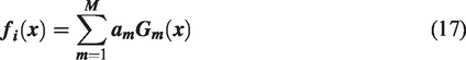
In this study, a training technique known as weak learning was used to develop a robust classifier using the AdaBoost method. The objective of weak learning was to identify the weak classifier that most effectively differentiates between positive and negative data. The optimal threshold value for each feature was determined through weak learning, ensuring that only a minimum number of cases are incorrectly categorized.⁴⁷ Equation (16) is used to calculate the weighting vector wn. The calculation of wn requires equations (14) and (15). In equation (14), Gi (xi) represents the weak classifier, and wn represents the observation weights, where i = 1, 2,…, N. Fi(x) is computed in equation (17) using equation (15) and the weak classifier value. The final classifier output, f, which represents the weighted linear combination of classifiers generated at each step of the process, is presented in equation (18).

$$\mathit{er}{\mathit{r}}_{\mathit{m}}=\frac{{\sum }_{\mathit{i}=1}^{\mathit{N}}{\mathit{w}}_{\mathit{i}}\mathit{I}\left({\mathit{y}}_{\mathit{i}}\ne {\mathit{G}}_{\mathit{i}}\left({\mathit{X}}_{\mathit{i}}\right)\right)}{{\sum }_{\mathit{i}=1}^{\mathit{N}}{\mathit{w}}_{\mathit{i}}}$$

(14)

$${\mathit{a}}_{\mathit{m}}=\mathit{log}\left(\frac{1-\mathit{er}{\mathit{r}}_{\mathit{t}}}{\mathit{er}{\mathit{r}}_{\mathit{t}}}\right)$$

(15)

$${\mathit{w}}_{\mathit{i}}\leftarrow {\mathit{w}}_{\mathit{i}}{\mathit{e}}^{\left({\mathit{a}}_{\mathit{t}}\mathit{I}\left({\mathit{y}}_{\mathit{i}}\ne {\mathit{G}}_{\mathit{t}}\left({\mathit{X}}_{\mathit{i}}\right)\right)\right)}$$

(16)

$${\mathit{f}}_{\mathit{i}}\left(\mathit{x}\right)=\sum _{\mathit{m}=1}^{\mathit{M}}{\mathit{a}}_{\mathit{m}}{\mathit{G}}_{\mathit{m}}\left(\mathit{x}\right)$$

(17)

$$\mathit{f}=\mathit{sign}\left({\mathit{f}}_{\mathit{M}}\left(\mathit{x}\right)\right)$$

(18)

MLP

A neural network known as MLP generates a distinct vector for each set of inputs. The structure of MLP consists of an input layer, a hidden layer, and an output layer. The input layer of MLP is represented by equation (19).

$${\mathit{a}}^{\mathit{x}}=\mathit{x}$$

(19)

$${\mathit{a}}^{\mathit{l}+1}=\mathit{\Psi }\left({\mathit{w}}^{\mathit{l}}{\mathit{a}}^{\mathit{l}}+{\mathit{b}}^{\mathit{l}}\right)$$

(20)

According to equation (19), x is the input and a1 is the output of the network’s first layer. The input for each subsequent layer is the weighted output of the previous layer, as expressed in equation (20).

w(l) represents the weights of layer l, b(l) represents the bias in layer l, and Ψ denotes the nonlinear function used in this network. The function Ψ may be a hyperbolic tangent, sigmoid, or another type of activation function. Equation (21) represents the output layer of MLP.

$$h_{w,b}\left(x\right)=a^n$$

(21)

The weights are denoted by w, the bias by b, and the number of network layers by n. The objective function minimizes the discrepancy between the predicted and actual output, as shown in equation (22).

$$J\left(w,b;x,y\right)=\frac{1}{2}{\left|\left|h_{w,b}\left(x\right)-y\right|\right|}^2$$

(22)

LightGBM classifier

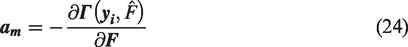
A scalable tree boosting engine known as XGBoost was introduced by Chen et al.⁴⁸ Despite XGBoost’s high accuracy, the LightGBM ensemble outperformed it in terms of time, computational efficiency, and robustness.⁴⁹ It was assumed that the dataset X = (xi, yi) has features x and label y. Equation (23) is derived using Γ(⋅) as a loss function and F0 as the initial fit optimization target.

$$\widehat{F}=\mathit{ar}{\mathit{g}}_{\mathit{F}}\mathit{min}{\mathit{X}}_{\mathit{x},\mathit{y}}[\mathit{\Gamma }\left(\mathit{y},\mathit{F}\left(\mathit{x}\right)\right]$$

(23)

The mth iteration of the pseudo residuals or gradient am, to which the decision tree hm(x) is fitted, is given by equation (24).

$${\mathit{a}}_{\mathit{m}}=-\frac{\partial \mathit{\Gamma }\left({\mathit{y}}_{\mathit{i}},\widehat{F}\right)}{\partial \mathit{F}}$$

(24)

The iterative criterion for Gradient Boosting Decision Trees (GBDT) to derive a new boosted fit aimed at reducing the loss function is given in equation (25). Here, λm serves as a multiplier, functioning as the step size, and is optimized using a linear search algorithm. The value of λm can be determined using equation (26).

$${\mathit{F}}_{\mathit{m}}\left(\mathit{x}\right)={\mathit{F}}_{\mathit{m}-1}\left(\mathit{x}\right)+{\mathit{\lambda }}_{\mathit{m}}{\mathit{h}}_{\mathit{m}}\left(\mathit{x}\right)$$

(25)

$${\mathit{\lambda }}_{\mathit{m}}=\mathit{ar}{\mathit{g}}_{\mathit{\lambda }}\mathit{m}\mathit{in}\sum _{\mathit{i}=1}^{\mathit{N}}\mathit{\Gamma }({\mathit{y}}_{\mathit{i}},{\mathit{F}}_{\mathit{m}-1}\left({\mathit{x}}_{\mathit{i}}\right)+\mathit{\lambda }{\mathit{h}}_{\mathit{m}}\left({\mathit{x}}_{\mathit{i}}\right))$$

(26)

Stratified K-fold cross-validation strategy

ML models trained on imbalanced biomedical datasets often exhibit biased performance when the class distribution is not preserved during model evaluation. In this study, the target variable, person_neoplasm_cancer_status, is moderately imbalanced. Because of this imbalance, a simple random train–test split can easily create folds in which cancer and noncancer cases are unevenly distributed. This imbalance can result in performance scores that are either unstable or unrealistically high. To ensure the robustness, reliability, and generalizability of each classifier, we employed stratified K-fold cross-validation, in which each fold preserves the original class proportions.

Specifically, we used a K = 10 stratified scheme for all classifiers. The dataset was divided into 10 separate folds, maintaining identical cancer/noncancer ratios within each fold. During evaluation, the model was iteratively trained on nine folds and tested on the remaining fold, ensuring that each instance was used once as part of the testing subset. This procedure produced 10 evaluation scores for each model. The final performance metrics, including accuracy, precision, recall, F1-score, and area under the curve (AUC), were calculated as the mean ± standard deviation across the 10 folds.

Hyperparameter optimization

Hyperparameters are predefined parameters for ML algorithms that control the operation of the models. In this study, GridSearchCV was used for hyperparameter tuning. Grid search with 10-fold cross-validation was implemented using GridSearchCV. This method tests the model with every possible combination of the specified parameter values, ensuring that all configurations are explored. As a result, the most effective model is selected, achieving the highest accuracy across all hyperparameter combinations. The tuned parameter ranges and the optimal configurations for all models—including SVM, NB, KNN, AdaBoost, MLP, and LightGBM—are summarized in Table 3.

Table 3.

Summary of hyperparameter optimization for all classifiers.

Model	Tuned parameters	Best hyperparameters
Support Vector Machine	C ∈ {0.1, 0.2, 0.5}	C = 0.5
	γ ∈ {0.01, 0.02, 0.05}	γ = 0.01
	kernel = ‘rbf’	kernel = ‘rbf’
Gaussian Naive Bayes	var_smoothing ∈ {1e−9, 1e−8, 1e−7, 1e−6, 1e−5}	var_smoothing = 1e−9
k-nearest neighbors	n_neighbors ∈ {25, 35, 45, 55, 65}	n_neighbors = 25
	weights = ‘uniform’	metric = ‘chebyshev’
	metric = ‘chebyshev’
AdaBoost	n_estimators ∈ {80, 120, 160}	n_estimators = 120
	learning_rate ∈ {0.05, 0.1, 0.2}	learning_rate = 0.1
	algorithm = ‘SAMME’	algorithm = ‘SAMME’
Multilayer Perceptron	hidden_layer_sizes ∈ {(50,), (100,)}	hidden_layer_sizes = (50,)
	activation = relu	alpha = 0.0001
	solver = adam	activation = relu
	alpha ∈ {0.0001, 0.001}	solver = adam
	max_iter = 500	max_iter = 500
LightGBM	‘n_estimators': [200, 220, 240, 260],	n_estimators ∈ {220}
	‘learning_rate': [0.006, 0.007, 0.008],	learning_rate ∈ {0.007}
	‘max_depth': [6, 7, −1],	max_depth ∈ {6}
	‘num_leaves': [50, 60, 70],	num_leaves ∈ {60}
	‘min_data_in_leaf': [1, 2, 3, 4, 5],	min_data_in_leaf ∈ {4}
	‘feature_fraction': [0.95, 1.0],	feature_fraction ∈ {0.95}
	‘bagging_fraction': [0.95, 1.0],	bagging_fraction ∈ {0.95}
	‘bagging_freq': [1],	bagging_freq ∈ {1}
	‘reg_alpha': [0.0],
	‘reg_lambda': [0.0],
	‘boosting_type': [‘gbdt']

GBM: Gradient Boosting Machine.

Model explainability analysis

Model explainability is essential for improving confidence in ML models, facilitating debugging, and providing decision-makers with insightful information. Two popular techniques for interpreting model outputs are SHAP values and LIME.

SHAP values

SHAP values provide a single measure for evaluating the importance of features in each prediction by considering every possible feature combination. Derived from cooperative game theory, these values represent how much each feature contributes to the difference between the mean prediction and the model’s output.⁵⁰

The Shapley values for each feature in the input space are computed using the SHAP method. The Shapley value (ϕ_i) represents a feature’s average contribution across all possible coalitions. The Shapley value can be expressed mathematically as follows:

$$\varphi \left(f,S\right)=\sum _{T\subseteq S\setminus \left\{i\right\}}\frac{(T!(S-T-1)!}{S!}\left(f\right(T\cup \left\{i\right\})-f(T\left)\right)$$

(27)

Here, X represents the full set of input features, S denotes a coalition of features that excludes feature i, |S| denotes the magnitude of the coalition, and f(S U i) denotes the model’s output when all features in S and i are present. When only the features in S are available, the model’s output is represented by f(S). The Shapley value represents the average marginal contribution of feature i across all possible coalitions. The procedure for obtaining SHAP values from the ET model is outlined in Algorithm 2.

Positive SHAP values indicate features that increase the expected value above the mean, while negative values indicate features that decrease it below the mean. Analyzing SHAP values provides insight into how specific variables influence individual predictions as well as the model’s overall performance.

LIME. LIME provides interpretable explanations tailored for specific data points, offering insight into complex models. It works by approximating the model locally around a particular data point and highlighting how each feature contributes to the final prediction. Rather than attempting to interpret the entire model at once, LIME focuses on analyzing the decision-making process for a single instance.⁵¹ The procedure for generating LIME explanations for a single instance is described in Algorithm 3.

Results and model explainability

This section presents the performance and explainability of the model. It describes the environment setup and reports the model’s accuracy, precision, recall, F1-score, and confusion matrix. Finally, model explainability ensures the transparency and reliability of the predictions by providing insights into how the model makes decisions.

Environment setup

For conducting this research, certain resources were required. The proposed model was developed using the resources listed in Table 4.

Table 4.

Environment setup of the proposed system.

Resource	Details
CPU	Intel® Core™ i-7- 13700 K CPU @ 3.20 GHz
RAM	16 GB
GPU	Intel® UHD Graphics
Experimental tool	Google Colab

CPU: central processing unit; RAM: random access memory; GPU: graphics processing unit.

Evaluation matrix

A confusion matrix (N × N) is used to quantify ML classification, where N represents the number of target classes. By summarizing the number of accurate and inaccurate predictions, this technique identifies the most effective ML classifiers. It evaluates each classifier’s performance on positive and negative classes, with two categories indicating correct predictions and two indicating incorrect predictions: true positive (TP), true negative (TN), false positive (FP), and false negative (FN).⁵² Next, the metric formulas, i.e. equations (28) to (31), are used to assess each classifier. This section presents an evaluation and comparison of the classifiers. The confusion matrix of each classifier is shown in Figure 5.

$$\mathit{Accuracy}=\frac{(\mathit{TP}+\mathit{TN})}{(\mathit{TP}+\mathit{FP}+\mathit{FN}+\mathit{TN})}$$

(28)

$$\mathit{Precision}=\frac{\mathit{TP}}{(\mathit{TP}+\mathit{TN})}$$

(29)

$$\mathit{Recall}=\frac{\mathit{TP}}{(\mathit{TP}+\mathit{FN})}$$

(30)

$$\mathit{F}1–\mathit{score}=\frac{2\times \mathit{Recall}\times \mathit{Precision}}{\mathit{Recall}+\mathit{Precision}}$$

(31)

Figure 5.

Confusion matrix for (a) Support Vector Machine, (b) Naïve Bayes, (c) K-Nearest Neighbor, (d) AdaBoost, (e) Multilayer Perceptron, and (f) Light Gradient Boosting Machine.

The performance of each classifier was evaluated based on the criteria described above, both before and after hyperparameter optimization. The results are summarized in Tables 5 and 6.

Table 5.

Assessment of classification techniques before optimization.

Model	Precision	Recall	F1-score	Accuracy (%)
Support Vector classifier	0.66	0.65	0.54	65.37
Naive Bayes classifier	0.84	0.84	0.84	82.55
KNN classifier	1.00	1.00	1.00	99.74
AdaBoost classifier	0.94	0.92	0.93	93.97
Multilayer Perceptron	0.79	0.68	0.58	70.13
LightGBM classifier	1.00	1.00	1.00	99.87

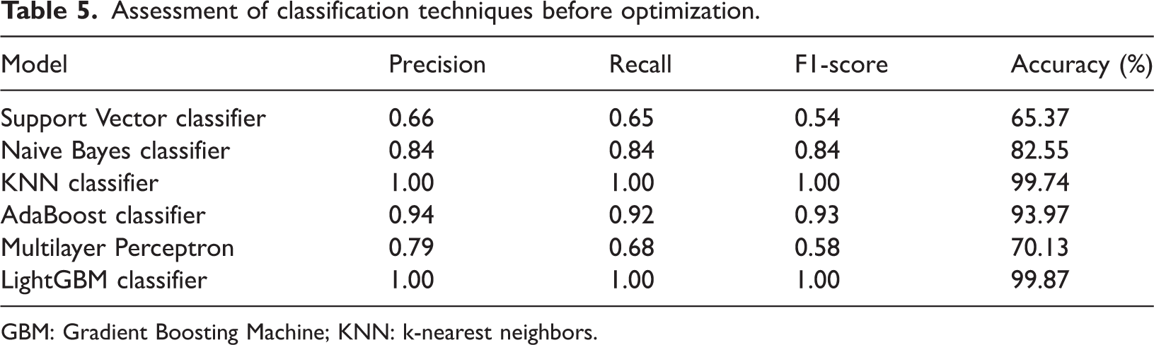
GBM: Gradient Boosting Machine; KNN: k-nearest neighbors.

Before optimization (Table 5), several models—particularly KNN and LightGBM—achieved very high accuracy (99.74% and 99.87%, respectively), demonstrating their ability to capture underlying data patterns even with default settings. In contrast, models such as SVM and MLP showed poor performance, with lower F1 scores and an imbalanced trade-off between precision and recall. These differences underscore the importance of hyperparameter tuning for achieving consistent and generalizable performance across classifiers.

After optimization (Table 6), most models demonstrated clear improvements. SVM showed notable gains in precision, recall, and F1 score, while NB improved marginally, achieving a better balance between precision and recall. KNN and AdaBoost remained strong, with tuning further stabilizing their performance. LightGBM continued to be the top-performing model, maintaining near-perfect accuracy after tuning. In contrast, MLP experienced a slight decline, reflecting its sensitivity to parameter settings and data characteristics.

Table 6.

Assessment of classification techniques after optimization.

Model	Precision	Recall	F1-score	Accuracy (%)
Support Vector classifier	0.863	0.826	0.808	82.56
Naive Bayes classifier	0.836	0.832	0.819	83.19
KNN classifier	0.945	0.944	0.943	94.35
AdaBoost classifier	0.926	0.926	0.925	92.60
Multilayer Perceptron	0.682	0.649	0.529	64.87
LightGBM classifier	0.998	0.997	0.997	99.74

GBM: Gradient Boosting Machine; KNN: k-nearest neighbors.

When evaluated using stratified cross-validation, LightGBM showed a minor reduction in accuracy, reflecting a shift from the optimistic single-split estimate to a more realistic performance range. A similar pattern was observed for KNN, whose very high baseline accuracy (99.74%) decreased slightly to a more stable value, indicating its sensitivity to neighborhood structure and inherent variance. Figure 6 illustrates the comparison of model accuracies before and after optimization, highlighting the improvements achieved through hyperparameter tuning.

Figure 6.

Comparison of model accuracy before and after optimization.

AU-ROC of different models

The ROC curve provides a summary of a classification model’s performance across all classification thresholds. The performance of our ML classifier—optimized using hyperparameter tuning and evaluated through 10-fold cross-validation—is illustrated in the AU-ROC curve shown in Figure 7. ROC analysis evaluates the sensitivity and specificity of binary classifiers. The AUC measures the degree of separability, while the ROC represents a probability curve.⁵³ It demonstrates how well the model can differentiate between classes.

$$\mathbf{TPR} \left(\mathbf{Sensitivity}\right)=\frac{\mathit{TP}}{\mathit{TP}+\mathit{FN}}$$

(32)

$$\mathbf{FPR} (\mathbf{1}-\mathbf{Specificity})=\frac{\mathit{FP}}{\mathit{TN}+\mathit{FP}}$$

(33)

Figure 7.

ROC curve for (a) Naïve Bayes, (b) k-nearest neighbor, (c) AdaBoost, (d) Multilayer Perceptron, and (e) Light Gradient Boosting Machine. ROC: receiver operating characteristic.

A higher AUC indicates that the model is better at distinguishing between patients who have the condition and those who do not. In the ROC curve, the true positive rate (TPR) is plotted on the Y-axis and the false positive rate (FPR) on the X-axis.

When AUC = 1, the classifier can correctly distinguish all positive and negative class points.⁵⁴ Conversely, when AUC = 0, the classifier would predict all negatives as positives and all positives as negatives. When 0.5 < AUC < 1, the classifier has a good probability of distinguishing between positive and negative class values. When the AUC is less than 0.5, the classifier cannot differentiate between positive and negative class points. Therefore, a classifier’s AUC score increases with its ability to discriminate between positive and negative classifications. This explains the evaluation process of the ROC curve for the hyperparameter-optimized classifier using 10-fold cross-validation.

Explainablity analysis

This section discusses the model’s performance, the factors influencing its prediction for a particular class, and the values that contribute to this outcome. The model’s predictions are explained using SHAP and LIME.

SHAP values

The SHAP summary plots are shown in Figure 8(a), illustrating the contribution of features from the EC dataset. The Light Gradient Boosting Machine (LGBM) classifier generates the SHAP values, which quantify how individual features affect the prediction and rank them according to their importance. The Y-axis displays the ranked features, while the X-axis shows their corresponding SHAP values. The color of each dot represents the value of a specific feature instance, with each dot corresponding to one data point. Blue indicates lower feature values, and red indicates higher values. The horizontal position of a dot indicates whether a feature has a positive or negative impact on the model’s output. Positive SHAP values push predictions toward the positive class (e.g. higher cancer risk), whereas negative values push predictions in the opposite direction.

Figure 8.

SHAP summary plot and bar plot for LightGBM. (a) SHAP summary plot and (b) Bar plot of mean SHAP values. SHAP: Shapley Additive Explanations; LightGBM: Light Gradient Boosting Machine.

As shown in Figure 8(b), features such as vital_status, has_new_tumor_events_information, and days_to_last_followup have high SHAP values, indicating that they significantly influence the model’s predictions. Clinically, vital_status indicates whether the patient is alive or deceased, serving as a direct mortality indicator. days_to_last_followup represents the follow-up duration, often used as a surrogate for survival time. Similarly, has_new_tumor_events_information captures whether the patient has experienced tumor recurrence or progression, which is a key factor in prognosis. The presence of these features among the top contributors reinforces the clinical relevance of the model’s learned patterns.

LightGBM performance using SHAP-selected features

From the SHAP summary plot, the mean absolute SHAP value was calculated for each feature, quantifying its average contribution to the model’s predictions. All features were then ranked in descending order according to their mean |SHAP| scores, and the top-k most influential features were selected for further analysis.

The feature selection rule can be expressed as follows:

$$\mathbf{Top}–\mathbf{k}\hspace{0.17em}\mathbf{Features}=\mathbf{arg}\underset{\mathit{k}}{\mathbf{max}}\left(\mathit{Mean}\right|\mathit{SHA}{\mathit{P}}_{\mathit{i}}\left|\right)$$

In this study, selecting the top 20 SHAP features provided the best balance between model interpretability and predictive performance, ensuring that only the most clinically and statistically relevant variables were retained.

After selecting the top 20 SHAP features, the dimensionality of the dataset was substantially reduced, resulting in a more compact feature representation compared with the original full-feature set. Using this reduced SHAP-selected subset, the LightGBM classifier was retrained to assess whether a smaller yet highly informative group of predictors could maintain competitive performance. During model development, a stratified 10-fold cross-validation strategy was applied to ensure that the underlying class distribution remained consistent across all folds, which is essential when handling imbalanced or clinically sensitive datasets. Hyperparameter tuning was then conducted through an extensive GridSearchCV procedure, in which key LightGBM parameters—such as the number of boosting iterations, number of leaves, learning rate, tree depth, minimum data per leaf, and feature and bagging fractions—were systematically explored to identify the configuration yielding the most reliable performance. Accuracy was used as the evaluation metric, and the same experimental settings were applied to both the full-feature and SHAP-selected models to allow a direct and unbiased comparison. The retraining pipeline therefore consisted of reducing the dataset to the SHAP-derived feature subset, performing stratified cross-validation, identifying optimal hyperparameters through grid search, selecting the best estimator, and finally evaluating the model on the corresponding reduced test set features.

The comparison presented in Table 7 shows that the SHAP-selected top-20 feature model maintains performance comparable to the full-feature LightGBM model. Using only the 20 SHAP-selected features, the LightGBM model achieved accuracy (99.76%) similar to the full-feature model (99.74%). This indicates that dimensionality reduction did not compromise performance and instead produced a more efficient and interpretable classifier.

Table 7.

Comparison of LightGBM performance: full vs. SHAP-selected features.

Model variant	Feature count	Cross-validation strategy	Best accuracy (test set)
Full-feature LightGBM (Untuned)	31	–	99.87%
Full-feature LightGBM (Tuned)	31	Stratified 10-fold +hyperparameter tuning	99.74%
SHAP-selected LightGBM (Top 20 features)	20	Stratified 10-fold + hyperparameter tuning	99.76%

GBM: Gradient Boosting Machine; SHAP: Shapley Additive Explanations.

LIME explainability

To complement the SHAP-based interpretability study, a global feature importance analysis was conducted using LIME. Although LIME is primarily a local explanation technique, global importance can be derived by aggregating feature contributions across multiple perturbed samples. Using the tuned LightGBM model, global LIME importance scores were computed and ranked in descending order. Figure 9 shows the global LIME feature importance, highlighting the most influential features based on aggregated LIME weights.

Figure 9.

Global LIME feature importance. LIME: Local Interpretable Model-Agnostic Explanations.

The results indicate that vital_status, has_new_tumor_events_information, and stage_event_pathologic_stage have the highest global contributions, suggesting their strong influence on overall model predictions. The top-ranked LIME global importance values are as follows: vital_status (0.2533), has_new_tumor_events_information (0.1553), stage_event_pathologic_stage (0.0900), primary_pathology_karnofsky_performance_score (0.0471), and city_of_procurement (0.0395). These variables dominate the model’s decision-making, and the LIME-derived importance pattern aligns with known clinical indicators of cancer progression, providing additional interpretability to the model.

LightGBM performance using LIME-selected features

Based on the global LIME ranking, the most important features were selected to form a reduced LIME-based feature subset. These influential variables were used to retrain the LightGBM classifier. The dataset was reconstructed using only the LIME-selected features, and the model was trained with stratified 10-fold cross-validation to maintain class balance. Hyperparameter tuning was performed using GridSearchCV, following the same settings applied to the full-feature and SHAP-based models. The final evaluation on the test set was performed using accuracy as the metric. The results showed that the LIME-based subset provides stable and competitive performance, indicating that a smaller and more interpretable feature set can achieve accuracy close to that of the full model.

Table 8 summarizes the comparative performance of two model configurations: the full-feature LightGBM model and the LIME-selected feature model. The LIME-based subset achieves high predictive accuracy despite substantial dimensionality reduction. Compared with the tuned full-feature model, the LIME-based model demonstrates competitive performance, although it is slightly lower due to its instance-based nature and less stable global ranking.

Table 8.

Comparison of LightGBM performance: full vs. LIME-selected features.

Model variant	Feature count	Cross-validation strategy	Best accuracy (test set)
Full-feature LightGBM (Untuned)	31	–	99.87%
Full-feature LightGBM (Tuned)	31	Stratified 10-fold + hyperparameter tuning	99.74%
LIME-selected LightGBM (Top 20 features)	20	Stratified 10-fold + hyperparameter tuning	99.62%

GBM: Gradient Boosting Machine; Local Interpretable Model-Agnostic Explanations.

Comparative explainability analysis: SHAP vs. LIME (global)

SHAP and LIME were compared to understand how both methods explain the LightGBM model at the global level. SHAP provides importance scores based on the model’s internal structure, whereas LIME estimates importance by locally approximating model behavior and aggregating the results. Both methods identified several common high-impact clinical features, indicating consistency in detecting the key predictors.

To evaluate the effect of these selected features on model performance, LightGBM was retrained using the top 20 features chosen separately by SHAP and LIME. The training procedure followed the same setup as the full-feature model, including stratified 10-fold cross-validation and identical hyperparameter tuning. As shown in Table 9, the SHAP-selected feature subset achieved accuracy nearly equal to that of the full model, while the LIME-selected subset also produced strong performance with only a small reduction. These results demonstrate that both SHAP and LIME can provide compact and informative feature sets without substantial loss of predictive accuracy.

Table 9.

Comparison of LightGBM performance using global SHAP and LIME.

Model variant	Feature count	Cross-validation strategy	Best accuracy (test set)
Full-feature LightGBM (Tuned)	31	Stratified 10-fold + hyperparameter tuning	99.74%
SHAP-selected LightGBM (Top 20 features)	20	Stratified 10-fold + hyperparameter tuning	99.76%
LIME-selected LightGBM (Top 20 features)	20	Stratified 10-fold + hyperparameter tuning	99.62%

GBM: Gradient Boosting Machine; Local Interpretable Model-Agnostic Explanations; SHAP: Shapley Additive Explanations.

Comparative explainability analysis: SHAP vs LIME (local)

1. Local explainability for a noncancer prediction

For the selected test instance, the LightGBM model predicted no cancer with a confidence of 99.72% (Figure 10(a) and (b)). This high certainty aligns with the local interpretability results provided by LIME and SHAP. As shown in Figure 10(a), the LIME explanation for the cancer class indicates that features such as vital_status and has_new_tumor_events_information exert a positive influence toward cancer (red bars), whereas features such as days_to_last_followup, stage_event_pathologic_stage, and stage_event_tnm_categories strongly oppose cancer (green bars). The cumulative negative contributions dominate, supporting the model’s decision for no cancer. Similarly, the SHAP force plot in Figure 10(b) illustrates that the overall prediction score is shifted far to the negative side (f(x) = −6.32), primarily due to strong negative contributions from has_new_tumor_events_information, vital_status, and stage_event_tnm_categories. Although age_began_smoking_in_years provides a minor positive push toward cancer, its effect is outweighed by the opposing features. Both methods consistently highlight clinically relevant factors, confirming that the model’s prediction is not arbitrary but grounded in interpretable feature influences.

Figure 10.

Comparative local explainability for a noncancer prediction: LIME vs. SHAP. (a) Local explanation using LIME for the selected instance and (b) Local explanation using SHAP force plot for the selected instance. LIME: Local Interpretable Model-Agnostic Explanations; SHAP: Shapley Additive Explanations.

2. Local explainability for a cancer prediction

For the selected test instance, the LightGBM model predicted cancer with a confidence of 99.73% (Figure 11(a) and (b)). The LIME explanation in Figure 11(a) highlights feature contributions toward the cancer class: has_new_tumor_events_information, stage_event_pathologic_stage, and age_began_smoking_in_years exert strong positive influence (red bars), pushing the prediction toward cancer. Although vital_status shows a green bar indicating a slight opposing effect, its magnitude is insufficient to counterbalance the dominant red contributions. Similarly, the SHAP force plot in Figure 11(b) shows that the overall prediction score is shifted far to the positive side (f(x) = +5.90), confirming a strong inclination toward cancer. Key features such as vital_status = 1.0, stage_event_tnm_categories = 26.0, and primary_pathology_residual_tumor > 0 appear in red, signifying their substantial positive impact on the model’s output. Both interpretability methods consistently reveal clinically relevant factors that justify the model’s decision, reinforcing the transparency and reliability of the prediction.

Figure 11.

Comparative local explainability for a cancer prediction: LIME vs. SHAP. (a) Local explanation using LIME for the selected instance and (b) Local explanation using SHAP force plot for the selected instance. LIME: Local Interpretable Model-Agnostic Explanations; SHAP: Shapley Additive Explanations.

Comparison with others works

Numerous scholars have investigated EC in recent years and proposed various strategies and methodologies, resulting in diverse and sometimes conflicting findings. Consequently, we were motivated to address this disease to overcome existing constraints.

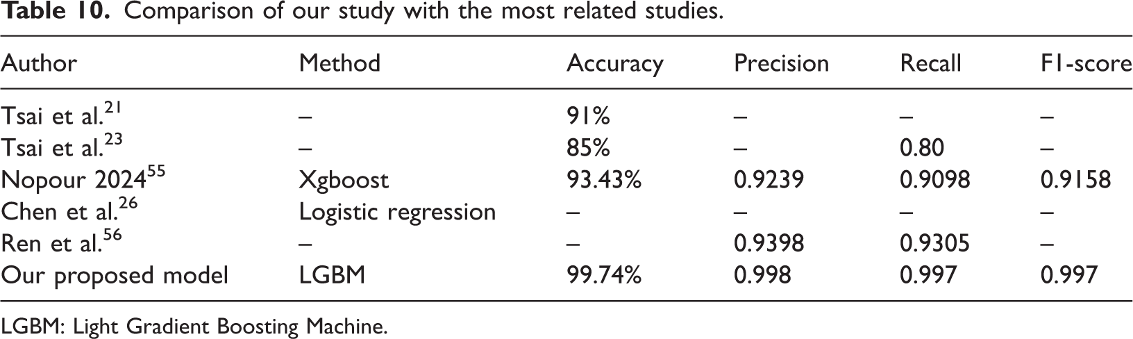
Table 10 presents a comparison between our proposed model and several existing methods reported in related studies. The comparison is based on four evaluation metrics: accuracy, precision, recall, and F1-score. As shown in the table, the method proposed by Tsai et al.²¹ achieved an accuracy of 91%, while Tsai et al.²³ reported an accuracy of 85% with a recall of 0.80. Nopour (2024)⁵⁵ employed the XGBoost algorithm and achieved an accuracy of 93.43%, a precision of 0.9239, a recall of 0.9098, and an F1-score of 0.9158. Chen et al.²⁶ applied logistic regression but did not report any performance metrics. Ren et al.⁵⁶ reported precision and recall values of 0.9398 and 0.9305, respectively.

Table 10.

Comparison of our study with the most related studies.

Author	Method	Accuracy	Precision	Recall	F1-score
Tsai et al. 21	–	91%	–	–	–
Tsai et al. 23	–	85%	–	0.80	–
Nopour 2024 55	Xgboost	93.43%	0.9239	0.9098	0.9158
Chen et al. 26	Logistic regression	–	–	–	–
Ren et al. 56	–	–	0.9398	0.9305	–
Our proposed model	LGBM	99.74%	0.998	0.997	0.997

LGBM: Light Gradient Boosting Machine.

Although Table 10 shows that our proposed LightGBM model achieved the highest accuracy (99.74%) with nearly perfect precision, recall, and F1-scores, it is important to note that the compared studies differ substantially in their experimental setup, dataset characteristics, and data modalities. For example, Tsai et al. employed hyperspectral imaging data, whereas our study utilized structured clinical data from the Kaggle EC dataset. Therefore, this comparison should not be interpreted as a direct benchmark but rather as a contextual illustration of the potential of our LightGBM framework to perform competitively across different methodological paradigms for EC prediction.

Conclusion

ML provides robust tools for analyzing large clinical datasets and supporting early disease detection. EC, one of the most aggressive malignancies worldwide, often remains undiagnosed until the late stages. In this study, six ML classifiers—SVM, Gaussian NB, KNN, AdaBoost, LightGBM, and MLP—were applied to develop an accurate EC prediction model. After preprocessing and MI-based feature selection, 31 key clinical features were retained. Using a standardized workflow with stratified 10-fold cross-validation and hyperparameter tuning, LightGBM achieved the best performance, reaching up to 99.87% accuracy before tuning and 99.74% after cross-validation, along with nearly perfect precision, recall, F1-score, and AUC.

A major strength of this work is its strong model interpretability. SHAP provided global insight into the most influential clinical factors, while LIME explained individual predictions. Both methods showed consistency and confirmed the model’s clinical relevance. Feature reduction experiments using SHAP/LIME-selected features also maintained high accuracy (SHAP: 99.76%, LIME: 99.62%), indicating that the model remains effective even with fewer predictors.

This study is limited by the use of a single open-source dataset with restricted demographic diversity, which may affect generalizability. Future research will include larger, multicenter datasets and additional data types, such as imaging. We also plan to develop a user-friendly web-based decision-support tool to provide real-time EC risk prediction for healthcare professionals.