Estimating the Expected Value of Sample Information Using the Probabilistic Sensitivity Analysis Sample

Abstract

Health economic decision-analytic models are used to estimate the expected net benefits of competing decision options. The true values of the input parameters of such models are rarely known with certainty, and it is often useful to quantify the value to the decision maker of reducing uncertainty through collecting new data. In the context of a particular decision problem, the value of a proposed research design can be quantified by its expected value of sample information (EVSI). EVSI is commonly estimated via a 2-level Monte Carlo procedure in which plausible data sets are generated in an outer loop, and then, conditional on these, the parameters of the decision model are updated via Bayes rule and sampled in an inner loop. At each iteration of the inner loop, the decision model is evaluated. This is computationally demanding and may be difficult if the posterior distribution of the model parameters conditional on sampled data is hard to sample from. We describe a fast nonparametric regression-based method for estimating per-patient EVSI that requires only the probabilistic sensitivity analysis sample (i.e., the set of samples drawn from the joint distribution of the parameters and the corresponding net benefits). The method avoids the need to sample from the posterior distributions of the parameters and avoids the need to rerun the model. The only requirement is that sample data sets can be generated. The method is applicable with a model of any complexity and with any specification of model parameter distribution. We demonstrate in a case study the superior efficiency of the regression method over the 2-level Monte Carlo method.

Health economic decision-analytic models are used to estimate the expected net benefits of competing decision options. The true values of the input parameters of such models are rarely known with certainty, and uncertainty in model parameters typically results in decision uncertainty. This may motivate decision makers to consider options for further data collection alongside the adoption of new technologies or to delay adoption until after data collection.^1,2 The value of learning an input parameter (or a group of input parameters) can be quantified by its partial expected value of perfect information (partial EVPI).^3–6 However, we are unlikely to be able to collect perfect information, and it is more useful to quantify the value of specific research designs that will inform the decision-making problem. The value of reducing, rather than eliminating, uncertainty through the collection of data is captured by the expected value of sample information (EVSI).^4,7,8

The EVSI for any particular data collection exercise will depend not only on the study design in question but also on the decision context. ⁸ Important factors include whether there are costs associated with either delaying or reversing adoption decisions,^1,9,10 whether the adoption decision will be fully implemented ¹¹ and whether the proposed study extends across jurisdictions.^12,13 Some of these factors arise in moving from EVSI per patient to population EVSI, but others also arise in estimating EVSI per patient. While recognizing these issues, we do not discuss them further in this article but concentrate on the problem of computing per-person EVSI within a single jurisdiction under the assumption of costless reversibility with perfect implementation and with no delay in either the study or the adoption.

The concept of EVSI was first discussed in the health economics literature well over a decade ago.^4,7,14,15 Despite this, very few research funding or design decisions are informed by EVSI. This, at least in part, reflects the computational burden of calculating EVSI via generic Monte Carlo sampling-based methods. For example, in a recently published cost-effectiveness study, the authors noted that to compute EVSI without assuming an approximation that the model was linear, it would have taken 7.5 days. ¹⁶ In another example, the proposed EVSI analysis would have taken 37.5 days. ¹⁷ Clearly, computation times of this order are prohibitive.

The reason for the high computational cost of EVSI analysis is that, unless the model is of a certain form or unless certain parametric assumptions are made, a nested 2-level Monte Carlo scheme is required. In this scheme, plausible data sets are generated in an outer loop, and then conditional on each data set, samples are generated from the posterior distribution of the parameters in an inner loop. The model is run with each inner loop set of parameters to estimate the expected net benefits, conditional on the data sets that have been simulated in the outer loop. The computational cost arises primarily due to the repeated evaluation of the model within the inner loop but also due to the burden of repeated sampling in the inner loop. If the aim is to search over the study design space, then this problem is further compounded because EVSI itself must be repeatedly calculated. Another difficult arises with the 2-level Monte Carlo approach if the prior distribution of the model parameters is not conjugate to the data likelihood. In this case, generating the inner-loop samples will typically require Markov chain Monte Carlo (MCMC), and the repeated application of MCMC for each sampled data set adds to the computational burden.

A fast approximation scheme for the inner-loop step has been proposed,^18,19 but this method requires repeated evaluation of partial derivatives of the log posterior density function and therefore considerable time and effort writing the necessary computer code on the part of the analyst. Computationally cheaper single-loop approaches are sometimes available, but these rely either on the model being of a certain form^7,20,21 or on assumptions of Normality of the mean incremental net benefits. ¹ Fast single-loop methods also exist for computing partial EVPI for single parameters,^22,23 but these have not yet been extended to the computation of EVSI.

In this article, we present a method for calculating per-patient EVSI that avoids the nested 2-level scheme, requiring only the single set of sampled model inputs and corresponding model outputs (i.e., net benefits) that is generated in a standard probability sensitivity analysis (PSA). The method is based on a nonparametric regression of the net benefits on data samples that are generated conditional on the sampled input parameters in the PSA and follows closely the nonparametric regression method for computing partial EVPI described in Strong et al. ²⁴ The method makes no assumptions regarding the form of the model, does not require the use of MCMC, and does not require that the parameter prior is conjugate to the data likelihood. All that is required is that the data likelihood can be sampled (but not necessarily evaluated). The article is structured as follows. In the second section, we introduce the method and describe its general application. In the third section, we demonstrate the method in the case study model that was used for illustrative purposes in Ades et al., ⁷ and in the fourth section, we present results. We conclude with a short discussion.

Method

EVSI is the expected difference between the value of the optimal decision based on some sample of data, informative for some subset of inputs, and the value of the decision made only with prior information.^3,4,7 To express this, we first introduce some notation.

We assume that we are faced with D decision options, indexed d = 1, . . ., D, and have built a model NB(d, θ) that aims to predict the net benefit of decision option d given a vector of p input parameter values θ = (θ₁, . . ., θ _p ). The true values of the input parameters are assumed to be unknown, and we represent beliefs about the input parameters via their joint distribution p(θ). We index a sample drawn from the joint distribution of the parameters with a bracketed superscript, θ⁽ⁿ⁾, for sample draws n = 1, . . ., N.

We envisage that we can collect data that will be informative for some subset of parameters. We consider the (as yet uncollected) data as a vector of random variables and denote this as uppercase X. We use lowercase x for some arbitrary realized (or sampled) vector of values from the distribution of X. We use the bracketed superscript notation to index a sample of data vectors x⁽ⁿ⁾, n = 1, . . ., N.

We denote the expectation over the joint distribution of θ as ${\mathbb{E}}_{\mathbf{\theta }}$ . We denote the expectation over the distribution of the data X as ${\mathbb{E}}_{\mathbf{X}}$ and over the posterior distribution of θ given data X as ${\mathbb{E}}_{\mathbf{\theta }\mathbf{|}\mathbf{X}}$ .

The expected value of our optimal decision, made only with current information is

$$\underset{d}{max}{\mathbb{E}}_{\mathbf{\theta }}\{\mathrm{NB}(d,\mathbf{\theta })\}.$$

If we had data X that were informative for (some subset of) the inputs, then the optimal decision would be that with the greatest net benefit, after averaging over the joint distribution of the inputs conditional on the data, p(θ|X). The expected net benefit would be

$$\underset{d}{max}{\mathbb{E}}_{\mathbf{\theta }|\mathbf{X}}\{\mathrm{NB}(d,\mathbf{\theta })\}.$$

But, since X is uncollected, we must average over possible data sets,

$${\mathbb{E}}_{\mathbf{X}}\left[\underset{d}{max}{\mathbb{E}}_{\mathbf{\theta }|\mathbf{X}}\{\mathrm{NB}(d,\mathbf{\theta })\}\right].$$

The distribution of X can be obtained by the marginalization of p(X, θ) = p(X|θ)p(θ), which suggests a straightforward Monte Carlo sampling scheme for X, that is, sample first a value θ* from the prior p(θ) and then sample X from the data likelihood p(X|θ = θ*). Note that the data likelihood will depend on the design of the study under consideration, and we return to this point when we discuss our case study. The EVSI is then the difference between equation (3) and equation (1),

$$\mathrm{EVSI}={\mathbb{E}}_{\mathbf{X}}\left[\underset{d}{max}{\mathbb{E}}_{\mathbf{\theta }|\mathbf{X}}\{\mathrm{NB}(d,\mathbf{\theta })\}\right]-\underset{d}{max}{\mathbb{E}}_{\mathbf{\theta }}\{\mathrm{NB}(d,\mathbf{\theta })\}.$$

At this point, we note that we can reexpress (4) as

$$\mathrm{EVSI}={\mathbb{E}}_{\mathbf{X}}\left[\underset{d}{max}{\mathbb{E}}_{\mathbf{\theta }|\mathbf{X}}\{\mathrm{NB}(d,\mathbf{\theta })\}\right]-\underset{d}{max}{\mathbb{E}}_{\mathbf{X}}[{\mathbb{E}}_{\mathbf{\theta }|\mathbf{X}}\{\mathrm{NB}(d,\mathbf{\theta })\}].$$

The reason for the reexpression will become apparent when we discuss Monte Carlo sampling schemes for estimating EVSI.

The Monte Carlo Approach to Computing EVSI

A probabilistic sensitivity analysis (PSA) takes N samples from the joint distribution of the input parameters, {θ⁽¹⁾, . . ., θ^(N)}, and generates a corresponding set of N net benefits {NB(d, θ⁽¹⁾), . . ., NB(d, θ^(N))} for each decision option d. From this, the usual Monte Carlo solution to the second term in equation (4) is

$$\underset{d}{max}{\mathbb{E}}_{\mathbf{\theta }}\{\mathrm{NB}(d,\mathbf{\theta })\}\approx \underset{d}{max}\frac{1}{N}\sum _{n=1}^N\mathrm{NB}(d,{\mathbf{\theta }}^{(n)}).$$

The first term in equation (4) requires more work, and unless there are analytic solutions to the expectations, the usual approach is to use a nested 2-level Monte Carlo method. ⁷ Here, the estimator is given by

$${\mathbb{E}}_{\mathbf{X}}\left[\underset{d}{max}{\mathbb{E}}_{\mathbf{\theta }|\mathbf{X}}\{\mathrm{NB}(d,\mathbf{\theta })\}\right]\simeq \frac{1}{K}\sum _{k=1}^K\underset{d}{max}\frac{1}{J}\sum _{j=1}^J\mathrm{NB}(d,{\mathbf{\theta }}^{(j,k)}),$$

where θ^(j,k) are samples drawn from the posterior distribution of θ|x^(k), and x^(k) are generated by first sampling θ^(k) from p(θ) and then x^(k) from p(X|θ = θ^(k)). Subtracting equation (6) from equation (7) results in the 2-level Monte Carlo EVSI estimator

$$\widehat{\mathrm{EVSI}}=\frac{1}{K}\sum _{k=1}^K\underset{d}{max}\frac{1}{J}\sum _{j=1}^J\mathrm{NB}(d,{\mathbf{\theta }}^{(j,k)})-\underset{d}{max}\frac{1}{N}\sum _{n=1}^N\mathrm{NB}(d,{\mathbf{\theta }}^{(n)}).$$

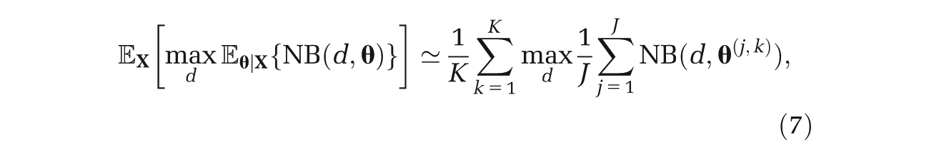
However, if we arrange our sampling scheme such that it reflects equation (5), we obtain instead

$$\widehat{\mathrm{EVSI}}=\frac{1}{K}\sum _{k=1}^K\underset{d}{max}\frac{1}{J}\sum _{j=1}^J\mathrm{NB}(d,{\mathbf{\theta }}^{\mathbf{(}\mathbf{j}\mathbf{,}\mathbf{k}\mathbf{)}})-\underset{d}{max}\frac{1}{K}\sum _{k=1}^K\frac{1}{J}\sum _{j=1}^J\mathrm{NB}(d,{\mathbf{\theta }}^{\mathbf{(}\mathbf{j}\mathbf{,}\mathbf{k}\mathbf{)}})$$

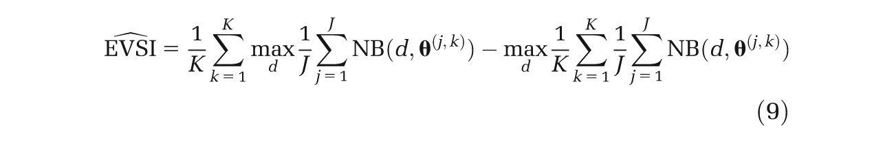
Here, both terms in the EVSI expression are evaluated using the same sampled values of θ, and hence we will obtain an estimator with smaller Monte Carlo error than if we were to use equation (8).

The first problem with the nested 2-level scheme is the requirement to evaluate the net benefit function (i.e., to run the model) at each iteration of the inner loop, resulting in J×K model evaluations. If the model is slow to run and/or if J and K are large (to obtain adequate precision), then the scheme will be computationally burdensome. A second potential problem is the requirement to sample from the posterior distribution of the input parameters, conditional on the sampled data, that is, obtaining the j = 1, . . ., J samples θ^(j,k) from each p(θ|x^(k)) in the inner loop. If p(X|θ) and p(θ) are conjugate, then the posterior distribution will be of a known form, and sampling from it will be straightforward. However, if conjugate forms are not appropriate, we may be required to resort to MCMC to generate the j = 1, . . ., J samples θ^(j,k) from p(θ|x^(k)). The MCMC step must be repeated for each of the k = 1, . . ., K sampled data values, and this will add considerably to the computational burden. Setting up the MCMC sampler (e.g., via writing BUGS code ²⁵ ) and checking the MCMC chain(s) for convergence also requires investment in modeler time.

We note at this point that in some restricted cases, we can avoid entirely the inner-loop Monte Carlo step. If the model is linear or multilinear (i.e., of “sum-product” form) in the parameters, and if the parameters are independent of one another (and retain this independence after updating with data), and if we can analytically compute the posterior expectations of the parameters given the data, then we can simply “plug in” the expected parameter values into the net benefit equation to obtain the expected net benefit.^7,21,26

Nonparametric Regression Method

The problem with the 2-level Monte Carlo scheme is the need to compute the inner expectation in the first term in equation (4) via Monte Carlo. Not only does this require J model runs for each outer loop, but it is this step that requires the potentially problematic sampling from the conditional distribution p(θ|X). We therefore propose to estimate this expectation as follows.

Consider generating a random parameter vector θ from p(θ) and a random data sample X conditional on θ and then evaluating NB(d, θ). We recognize that we can express the observed NB(d, θ) as a sum of the conditional expectation that we require and a mean-zero error term,

$$\mathrm{NB}(d,\mathbf{\theta }\mathbf{)}\mathbf{=}{\mathbb{E}}_{\mathbf{\theta }\mathbf{|}\mathbf{X}}\mathbf{\{}\mathrm{NB}\mathbf{(}\mathbf{d}\mathbf{,}\mathbf{\theta }\mathbf{)}\mathbf{\}}\mathbf{+}\mathbf{\epsilon },$$

where the error ϵ is a function of both X and θ.

To see why ϵ has zero mean, we rearrange to give

$$\epsilon =\mathrm{NB}(d,\mathbf{\theta })-{\mathbb{E}}_{\mathbf{\theta }|\mathbf{X}}\{\mathrm{NB}(d,\mathbf{\theta })\},$$

and then take expectations with respect to both X and θ, giving

$$\begin{array}{cc}\hfill {\mathbb{E}}_{\mathbf{X},\mathbf{\theta }}(\epsilon )\hfill & \hfill ={\mathbb{E}}_{\mathbf{X},\mathbf{\theta }}\{\mathrm{NB}(d,\mathbf{\theta })\}-{\mathbb{E}}_{\mathbf{X},\mathbf{\theta }}[{\mathbb{E}}_{\mathbf{\theta }|\mathbf{x}}\{\mathrm{NB}(d,\mathbf{\theta })\}]\hfill \\ \multicolumn{1}{c}{}& \hfill ={\mathbb{E}}_{\mathbf{\theta }}\{\mathrm{NB}(d,\mathbf{\theta })\}-{\mathbb{E}}_{\mathbf{X}}[{\mathbb{E}}_{\mathbf{\theta }|\mathbf{x}}\{\mathrm{NB}(d,\mathbf{\theta })\}],\hfill \end{array}$$

noticing that the first term in the right-hand side of equation (11) is a function only of θ and the second term a function only of X (θ having been integrated out). Then, by the law of total expectation (or “tower rule”), ${\mathbb{E}}_{\mathbf{X}}[{\mathbb{E}}_{\mathbf{\theta }|\mathbf{x}}\{\mathrm{NB}(d,\mathbf{\theta })\}]=\mathbb{E}\{\mathrm{NB}(d,\mathbf{\theta })\}$ , and hence $\mathbb{E}(\epsilon )=0$ . Note that this holds regardless of the distribution of θ and regardless of the relationship between θ and X.

Next, we recognize that the expectation ${\mathbb{E}}_{\mathbf{\theta }|\mathbf{X}}\{\mathrm{NB}(d,\mathbf{\theta })\}$ can be thought of as an unknown function of X. We denote this function g(d, X), and substituting this into equation (10) gives

$$\mathrm{NB}(d,\mathbf{\theta })=g(d,\mathbf{X})+\epsilon .$$

In some instances, the data X will be high dimensional (e.g., censored time-to-event data in a study that measures survival), and if this is so, we write the function g in terms of some low-dimensional summary statistic of the data T(X) = {T₁(X), . . ., T_p(X)}, giving

$$\mathrm{NB}(d,\mathbf{\theta })=g\{d,T(\mathbf{X})\}+\epsilon .$$

We discuss choice of summary statistic in the next section.

Last, for each decision option d = 1, . . ., D, we treat the net benefits in the PSA sample, NB(d, θ^(k)) as “noisy” data through which we can learn about the target function g{d, T(x^(k))} for k = 1, . . ., K. Thus, we can think of this as D regression problems. However, we immediately recognize that the target functions have unknown form, and we have no desire to impose any particular form. We could begin by fitting a standard linear model, with power and interaction terms to model the nonlinearity between the net benefits and the data, but we choose instead to adopt the more flexible “nonparametric” regression approach offered by the generalized additive model (GAM). GAM models assume that the expectation of the dependent variable is a smooth but usually unknown function of the independent variable, which is exactly what we need here. The standard linear model is a special case of the GAM model in which the functional form of the expectation of the dependent variable is specified a priori.

When we adopt a GAM model, we usually represent the unknown underlying smooth function as some form of spline, a common choice being the cubic spline. In the simplest case, a univariate cubic spline represents an arbitrary smooth single-input function as a series of short cubic polynomials joined piecewise such that the function is twice-differentiable at the “knots” (i.e., join points). The same spline can also be represented as the weighted sum of a series of predetermined “basis functions” that extend over the whole range of the function input. Simple univariate cubic splines have natural extensions to higher dimensions and to a regression framework, where the spline parameters (i.e., the basis function weights) are estimated from noisy data. For an introduction to GAM models, see Hastie and Tibshirani ²⁷ or Wood. ²⁸

Returning now to the problem of estimating g{d, T(X)}, we obtain the necessary “data” for the GAM regression analysis as follows. We assume we have at our disposal a PSA sample of size K. This consists of a set of k = 1, . . ., K samples from the distribution of the input parameters θ^(k), and k = 1, . . ., K corresponding evaluations of the model NB(d, θ^(k)), for each decision option d = 1, . . ., D. The dependent variable for regression d is the net benefit NB(d, θ^(k)) for decision option d. To generate realizations of the independent variable (which is common to all d = 1, . . ., D regression analyses), we sample, for each value θ^(k), a data set x^(k) from the likelihood p(X|θ = θ^(k)) and, from x^(k), calculate the summary statistic T(x^(k)). At no point do we attempt to derive or sample from the potentially difficult posterior distribution of the parameters, p(θ|x^(k)), and at no point do we rerun the economic model. This is why the method is fast and simple.

We note here that EVSI is invariant to the reexpression of net benefits as incremental net benefits, relative to some chosen “baseline” option. Under this reexpression, the (incremental) net benefit of the baseline option is zero. This reduces the number of regression equations from D to D− 1.

Choice of Summary Statistic T(·)

Study data x may be scalar or vector valued and may be informative for one or more economic model parameters. In the simplest case, we have scalar data that are informative for a single economic model parameter. Here we choose T(x) = x. If x is vector valued, but we still expect data only to update a single model parameter θ _i , and then we choose T(x) to be a sample estimator for θ _i . This leads to quite natural summary statistics. So, for example, if we wish to calculate the expected value of a 2-arm, binary outcome trial to update beliefs about an odds ratio, then we our choice of T(x) would be the sample odds ratio.

If we wish to update beliefs about q > 1 economic model parameters {θ₁, . . ., θ _q }, then we would calculate q summary statistics T(x) = {T₁(x), . . ., T_q(x)}, where each T_i(x) is a sample estimator for θ _i . For example, if we wish to calculate the expected value of a study to learn about the shape and scale parameters of a Weibull distribution, {θ₁, θ₂}, and x are censored time-to-event data, then we would choose {T₁(x), T₂(x)} to be the sample estimates $\{{\widehat{\theta }}_1,{\widehat{\theta }}_2\}$ derived from a Weibull survival model.

In the case of q > 1, we write the vector of scalar summary statistics as T(x) = {T₁(x), . . ., T_q(x)}, and fit the GAM model NB (d, θ) = g{d, T(x)} +ϵ, where g is now a multivariate smoothing function. ²⁸

Hypothetical Nonparametric Regression Example

To give an example, we imagine a hypothetical net benefit function NB(θ) = θ² (for clarity, we have dropped the decision option index d in this example). The parameter θ represents a proportion (e.g., of people in the population who have a certain characteristic), and current knowledge about the proportion is expressed via a Beta(40,200) distribution. We want to know the value of doing a study with 500 participants to learn about the proportion. The number of people in the study with the characteristic of interest, x, is modeled using a Binomial(θ, 500) distribution.

The PSA sample comprises samples {θ⁽¹⁾, . . ., θ^(K)} with the corresponding samples from the net benefit function {NB(θ⁽¹⁾), . . ., NB(θ^(K))}. For each sample θ^(k), we generate a sample of data x^(k) from X|θ^(k) ~ Binomial (θ^(k), 500). The data here are scalar, and we therefore choose T(x) = x. We fit a GAM regression of NB(θ) on T(x) and extract the fitted values, which are our estimates of ${\mathbb{E}}_{\mathbf{\theta }\mathbf{|}\mathbf{x}}\{\mathrm{NB}(\mathbf{\theta }\mathbf{)}\mathbf{\}}$ . In this hypothetical example, we can calculate ${\mathbb{E}}_{\mathbf{\theta }\mathbf{|}\mathbf{x}}\{\mathrm{NB}(\mathbf{\theta }\mathbf{)}\mathbf{\}}$ analytically, so can compare the GAM regression values with their true counterparts.

Figure 1 shows a scatter plot of sampled values of the incremental net benefit, NB(θ) = θ², versus sampled values of T(x). The two lines show the posterior expected net benefit ${\mathbb{E}}_{\mathbf{\theta }\mathbf{|}\mathbf{x}}\{\mathrm{NB}(\mathbf{\theta }\mathbf{)}\mathbf{\}}$ as a function of the sampled values of T(x). The solid line shows the GAM model fitted values, and the dashed line shows the analytically calculated values.

Figure 1

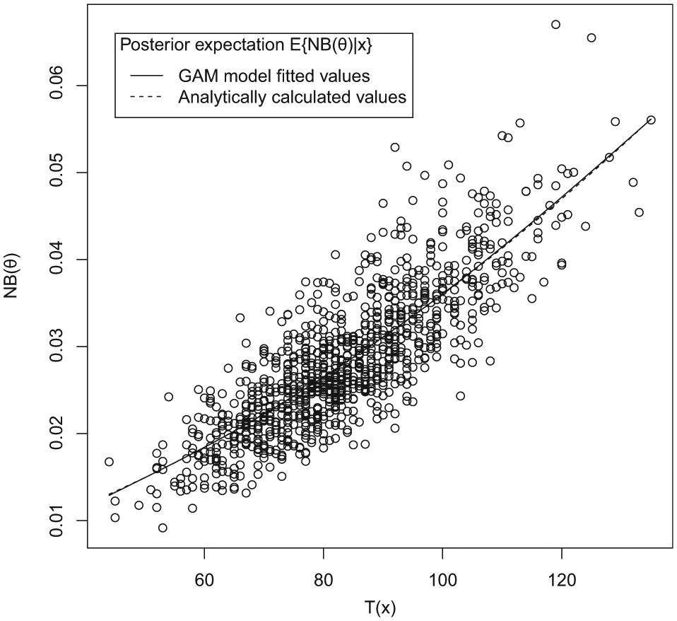
Hypothetical example. Generalized additive model (GAM) model fitted values of the posterior expected incremental net benefit versus analytic values. The lines representing the GAM fitted and analytic values are almost indistinguishable.

Regression Diagnostics

As with all regression analysis, it is important to check assumptions. Most important, we require that there is no structure in the residuals (e.g., a U-shaped or S-shaped pattern) since this would suggest unmodeled structure in the target function g and therefore bias in the fitted values. We note that for the purposes of calculating EVSI, we are seeking to estimate only the posterior mean net benefits. We do not require the posterior variance of the net benefits for the EVSI computation and therefore whether the residuals have equal variance and follow a particular distribution is of secondary importance. ²⁹

In contrast to the estimator for the EVSI, the estimator for the Monte Carlo standard error of the EVSI given in the online Appendix does rely on the net benefits having approximately equal variance and approximate Normality if the number of rows of the PSA is small. However, if the size of the PSA is large, then the standard error estimator can be justified on large sample results, even in the absence of Normality of the net benefits (see Appendix). ²⁸

EVSI Calculation

After fitting a GAM model for each decision option d, we then extract the regression model fitted values. The fitted values are estimates of g{d, T(x^(k))}, k = 1, . . ., K, our target quantity. We denote the GAM fitted values for decision option d as ${\hat{g}}_d^{(k)}$ , and the estimated EVSI is then given by

$$\widehat{\mathrm{EVSI}}=\frac{1}{N}\sum _{k=1}^N\underset{d}{max}{\hat{g}}_d^{(k)}-\underset{d}{max}\frac{1}{K}\sum _{k=1}^K{\hat{g}}_d^{(k)}.$$

Note that we choose $\underset{d}{max}\frac{1}{K}\sum _{k=1}^K{\hat{g}}_d^{(k)}$ rather than $\underset{d}{max}\frac{1}{K}\sum _{K=1}^K\mathrm{NB}(d,{\mathbf{\theta }}^{(k)})$ as the second term in the EVSI estimator, following expression (5) rather than expression (4). By choosing this as our estimator, we exploit the positive correlation between the two terms in equation (14) and hence estimate the EVSI with increased precision.

The sampling scheme for the GAM regression-based EVSI is given in Box 1.

Box 1

Generalized Additive Model (GAM) Regression-Based EVSI Algorithm

Generate a PSA sample of size K:  for k = 1, . . ., K do   Sample θ(k) from the distribution of the parameters, p(θ)   Evaluate the economic model to obtain (incremental) net benefits NB(d, θ(k))  end for Given the PSA sample, simulate data samples:  for k = 1, . . ., K do   Generate a data sample x(k) from p(X|θ(k))   Calculate summary statistic T(x(k))  end for Fit regression models and calculate EVSI:   Regress net benefits NB(d, θ(k)) from the PSA on T(x(k)) for each d   Extract GAM model fitted values for each d   Calculate EVSI via equation (14).

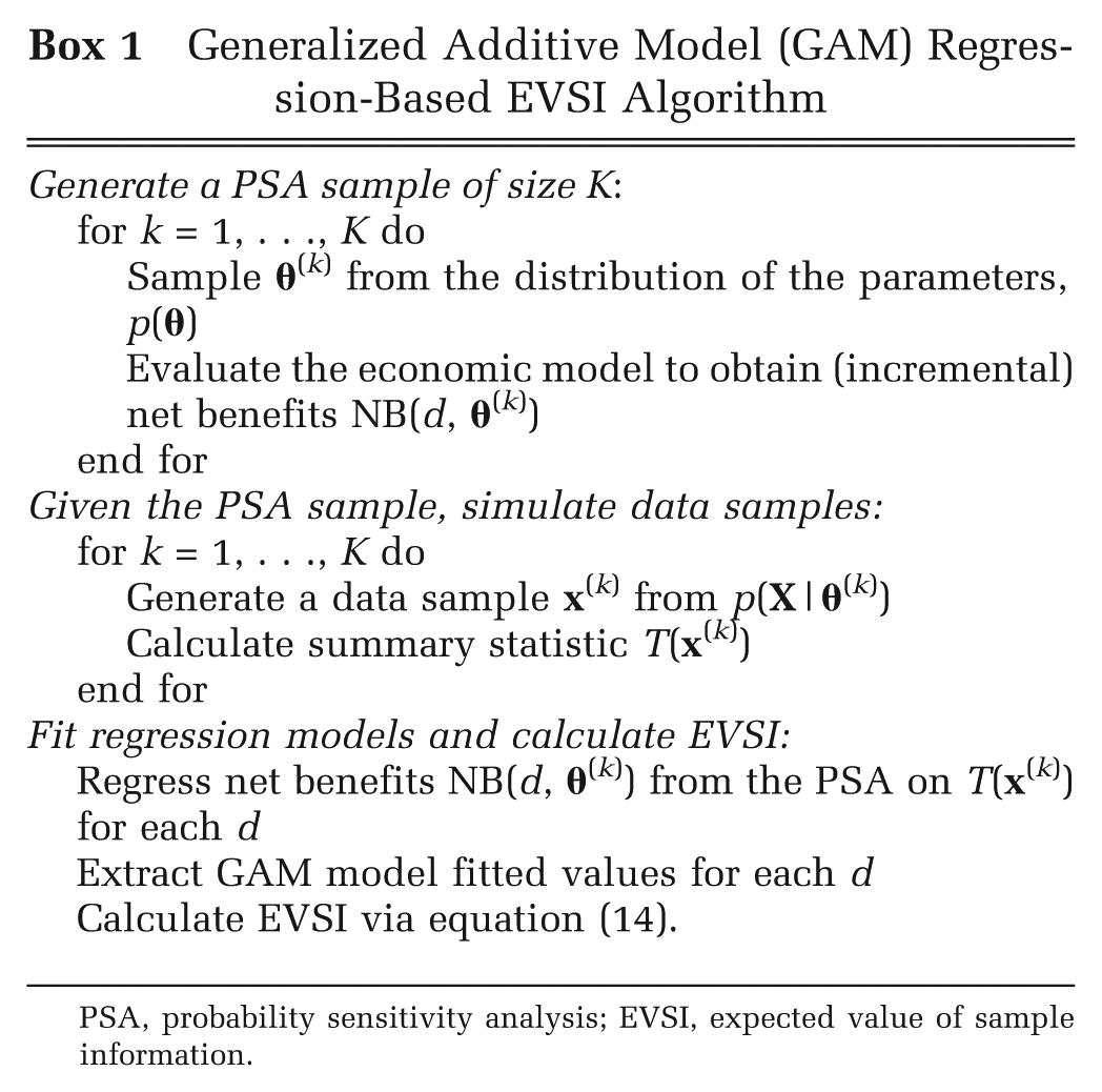
PSA, probability sensitivity analysis; EVSI, expected value of sample information.

Because we are averaging over k, we can think of this as a single-loop Monte Carlo method. The size of K will determine the precision of the estimate of the EVSI, and a method for estimating the standard error of the GAM-based approximation is given in the Appendix.

Case Study: Ades (2004) Decision Tree Model

Model

Our case study is based on the model that was used for illustrative purposes in Ades et al. ⁷ The decision problem has two options: d = 1 (standard care) and d = 2 (new treatment) and can be represented by a simple decision tree (Figure 2). There are 11 parameters in the model, which we write as the vector θ = (L, Q_E, Q_SE, C_E, C_T, C_SE, P_C, P_SE, OR, P_T, λ). Parameter definitions and distributions are given in Table 1. The output of the model is the net benefit for each decision option in monetary units. The algebraic form of the model is given in equations (15) and (16), with some components of θ being redundant in each net benefit function.

$$\mathrm{NB}(1,\mathbf{\theta })=P_C\{\lambda L(1+Q_E)/2-C_E\}+(1-P_C)\lambda L.$$

$$\begin{array}{cc}\multicolumn{1}{c}{\mathrm{NB}(2,\mathbf{\theta })=}& P_{\mathrm{SE}}{P}_T[\lambda \{L(1+Q_E)/2-Q_{\mathrm{SE}}\}-(C_T+C_{\mathrm{SE}}+C_E)]+\hfill \\ \multicolumn{1}{c}{P_{\mathrm{SE}}(1-P_T)\{\lambda (L-Q_{\mathrm{SE}})-(C_T+C_{\mathrm{SE}})\}+}\\ \multicolumn{1}{c}{(1-P_{\mathrm{SE}})P_T\{\lambda L(1+Q_E)/2-(C_T+C_E)\}+(1-P_{\mathrm{SE}})(1-P_T)(\lambda L-C_T).}\end{array}$$

Figure 2

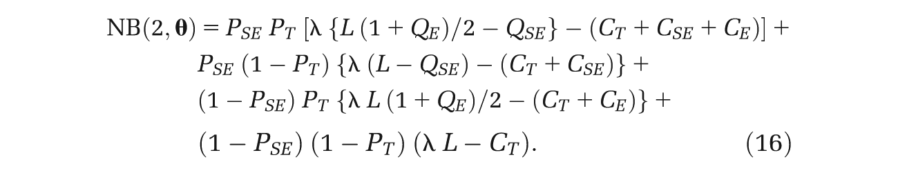
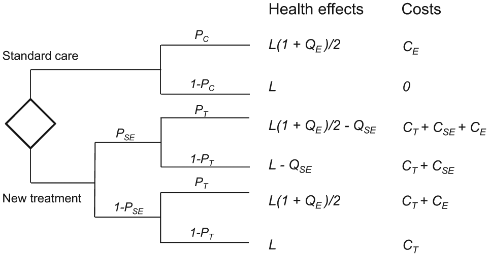
Decision tree model. From Ades et al., ⁷ copyright © 2004, Society for Medical Decision Making. Reprinted by Permission of SAGE Publishers.

Table 1

Case Study Parameter Distributions

Description	Parameter	Mean	Distribution
Mean remaining lifetime	L	30	Constant
QALY after critical event, per year	QE	0.6405	logit(QE) ∼N(0.6, 1/6)
QALY decrement due to side effects	QSE	1	Constant
Cost of critical event	CE	$200,000	Constant
Cost of treatment	CT	$15,000	Constant
Cost of treatment side effects	CSE	$100,000	Constant
Probability of critical event, no treatment	PC	0.15	Beta(15,85)
Probability of treatment side effects	PSE	0.25	Beta(3,9)
Odds ratio, (PT/(1 −PT ))/(PC / (1 −PC))	OR	0.2636	log(OR) ∼N(–1.5, 1/3)
Probability of critical event on treatment	PT	0.0440	[derived from OR and PC]
Monetary value of 1 QALY	λ	$75,000	Constant

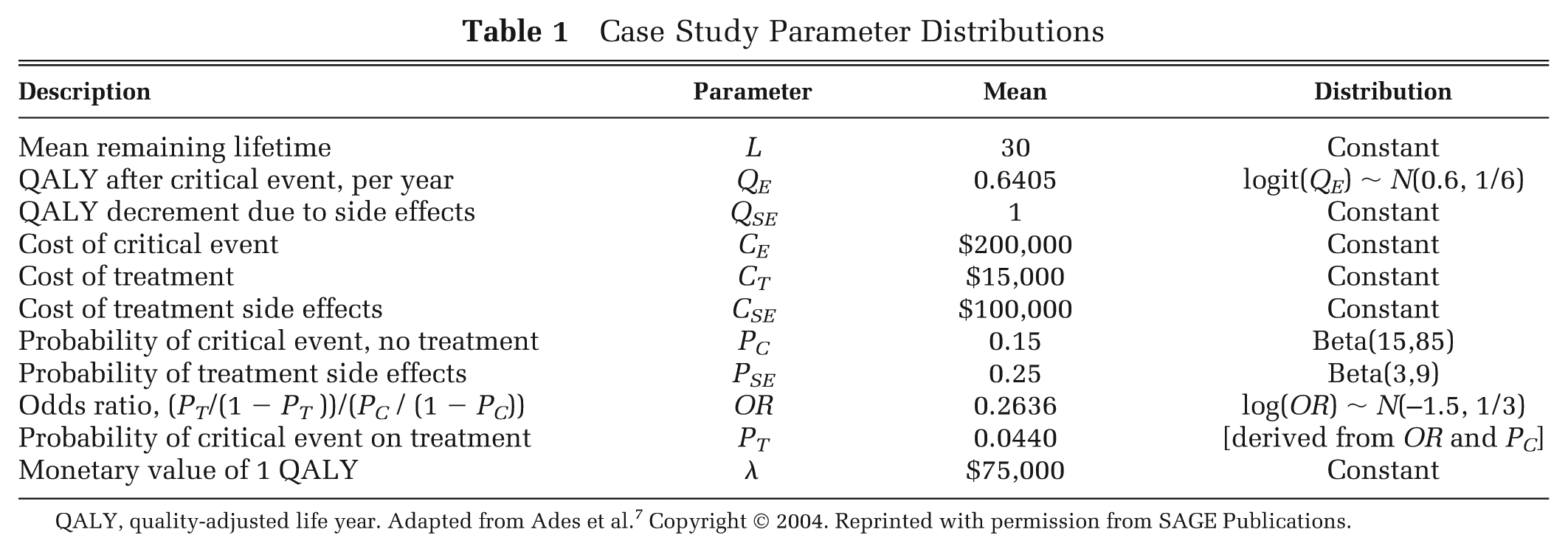
QALY, quality-adjusted life year. Adapted from Ades et al. ⁷ Copyright © 2004. Reprinted with permission from SAGE Publications.

The model is multilinear in the parameters, and all parameters are independent. Thus, the expectation of the net benefit, $\mathbb{E}\{\mathrm{NB}(d,\mathbf{\theta })\}$ , is equal to the net benefit equation evaluated at the parameter expectations, $\mathrm{NB}\{d,\mathbb{E}(\mathbf{\theta })\}$ . This is generally the case for decision tree models with independent parameters but not for Markov models or individual-level simulation models.

For our case study, we consider the same 3 data collection scenarios presented in Ades et al. ⁷ —that is, data collection to inform the probability of side effects (P_SE), the quality of life after critical event (Q_E), and the treatment effect size (OR). For each scenario, we calculated EVSI using 3 methods. First, we replicated the method presented in Ades et al. The method relies on the model being of multilinear form with independent parameters and that there are analytic solutions (or good approximations) to the posterior expectations of the parameters, conditional on simulated data. Hence, the method only requires a single-loop Monte Carlo scheme to evaluate the outer expectation in the first term in equation (4). Second, we used the 2-level Monte Carlo scheme outlined earlier, with an MCMC inner loop. This method does not rely on the model being multilinear with independent parameters or that there are analytic solutions to the posterior expectations of the parameters. However, it has high computational cost. Third, we used the GAM regression method presented earlier. As with the Ades et al. method, the GAM method uses Monte Carlo to evaluate the outer expectation in the first term in equation (4). For consistency, we use K to denote the size of the outer expectation Monte Carlo loop when reporting all 3 methods.

Because all 3 methods use Monte Carlo to estimate the outer expectation in equation (4), there will be a Monte Carlo sampling error that tends to zero as the outer-loop sampling size increases. For each estimated EVSI, we calculated the Monte Carlo standard error using the methods presented in the Appendix. We repeated each analysis with a range of values of K to demonstrate the relationship between K and the Monte Carlo standard error. We also recorded the total CPU time required to undertake the EVSI computation to compare the efficiency of each method at different values of K.

For the Ades et al. ⁷ method, we chose values of K equal to 10⁴, 10⁵, and 10⁶. For the MCMC-based method, we chose an inner-loop sample size of J = 10⁴ after an initial exploration to determine an adequate sample size to achieve stability of the inner-loop estimates. We then chose values of K equal to 10⁴, 10⁵, and 10⁶. Values of K greater than this required prohibitively long runtimes. For the GAM-based method, we chose values of K equal to 10⁴, 10⁵, and 10⁶.

Data Collection Scenario 1: EVSI for the Probability of Side Effects (P_SE)

To reduce uncertainty about P_SE, we considered the value of undertaking an observational study of n = 60 patients on the new treatment. The number of participants observed to experience a side effect is assumed to follow a Binomial(P_SE, 60) distribution.

Method 1—single-loop method presented in Ades et al

In method 1, we replicated the single-loop method used in the case study in Ades et al. ⁷ First, we drew k = 1, . . ., K samples from the Beta(3, 9) prior distribution for P_SE. Next, for each sampled value $P_{\mathrm{SE}}^{(k)}$ , we generated a sample of data x^(k) from a Binomial( $P_{\mathrm{SE}}^{(k)}$ , 60) distribution. Due to conjugacy, the posterior distribution has the closed form P_SE|x^(k) ~ Beta (3 +x^(k), 69 −x^(k)), with expectation ${\mathbb{E}}_{P_{\mathrm{SE}}|{\mathbf{x}}^{(k)}}(P_{\mathrm{SE}})=(3+{\mathbf{x}}^{(k)})/72$ . Because the economic model is multilinear in the parameters, we can calculate for each data set k the exact expected net benefit ${\mathbb{E}}_{\mathbf{\theta }|{\mathbf{x}}^{(k)}}\{\mathrm{NB}(d,\mathbf{\theta })\}$ by plugging into equations (15) and (16) the posterior expectation ${\mathbb{E}}_{P_{\mathrm{SE}}|{\mathbf{x}}^{(k)}}(P_{\mathrm{SE}})$ , along with the expected values for the remaining uncertain parameters, $\mathbb{E}(Q_E)$ , $\mathbb{E}(P_C)$ , and $\mathbb{E}(P_T)$ . Finally, we estimated the EVSI by

$$\widehat{\mathrm{EVSI}}=\frac{1}{K}\sum _{k=1}^K[\underset{d}{max}{\mathbb{E}}_{\mathbf{\theta }|{\mathbf{x}}^{(k)}}\{\mathrm{NB}(d,\mathbf{\theta })\}]-\underset{d}{max}\frac{1}{K}\sum _{k=1}^K[{\mathbb{E}}_{\mathbf{\theta }|{\mathbf{x}}^{(k)}}\{\mathrm{NB}(d,\mathbf{\theta })\}].$$

Method 2—2-level nested Monte Carlo/MCMC sampling scheme

In method 2, we implemented the generic 2-level Monte Carlo scheme outlined earlier. In an outer loop, we drew k = 1, . . ., K samples from the Beta(3, 9) prior distribution for P_SE. For each value $P_{\mathrm{SE}}^{(k)}$ , we generated a sample of data x^(k) from a Binomial( $P_{\mathrm{SE}}^{(k)}$ , 60) distribution. Conditional on each simulated trial data value x^(k), we then ran an inner-loop of size J = 10⁴. At each run of the inner loop, we sampled a vector of parameter values θ^(j,k) from the posterior distribution p(θ|x^(k)) and evaluated the model net benefit equation NB(d, θ^(j,k)). Finally, we calculated EVSI via equation (9). Because x^(k) is only informative for the parameter P_SE, and P_SE is independent of all other model parameters, drawing from p(θ|x^(k)) reduced in this case to drawing from the posterior distribution p(P_SE|x^(k)) and the prior distributions for the remaining parameters. Although the posterior distribution p(P_SE|x^(k)) has a known form in this example, we did not assume that this was so and implemented the inner loop in OpenBUGS. ²⁵ At each inner-loop step, we discarded the first 1000 MCMC samples as a burn-in.

Method 3—GAM regression

In method 3, we implemented the GAM regression scheme outlined earlier. First, we generated a PSA sample of size K. We calculated the incremental net benefit for each PSA sample. Next, for each parameter vector θ^(k) in the PSA sample, we generated a sample of data x^(k) from a Binomial( $P_{\mathrm{SE}}^{(k)}$ , 60) distribution. Because the data in this case are scalar, the summary statistic is T(x^(k)) = x^(k). We regressed the incremental net benefits on T(x^(k)), extracted the model-fitted values, and estimated the EVSI via equation (14).

Data Collection Scenario 2: EVSI for Quality of Life after Critical Event (Q_E)

To reduce uncertainty about Q_E, we considered the value of undertaking an observational study of n = 100 patients who have experienced a critical event. We assume that, conditional on Q_E, the sample mean of the logit transform of the quality of life reported in a single data collection exercise is Normally distributed with expectation logit(Q_E) and variance σ²/n, where σ², the population variance, is assumed known and equal to 2 (see Ades et al. ⁷ for details).

Method 1—single-loop method presented in Ades et al

As in scenario 1, we replicated the single-loop method used in the case study in Ades et al. ⁷ First, we drew k = 1, . . ., K samples from the Normal(0.6, 1/6) prior distribution for logit(Q_E). Next, for each sampled value logit(Q_E)^(k), we generated a sample of data x^(k) from a Normal{logit(Q_E)^(k), 1/50} distribution. Due to conjugacy, the posterior distribution of logit(Q_E)|x^(k) is Normal{(0.6 × 6 +x^(k)× 50)/(50 + 6),1/(50 + 6)}. The posterior expectation ${\mathbb{E}}_{Q_E|{\mathbf{x}}^{(k)}}(Q_E)$ can then be estimated from the posterior distribution of the logit-transformed parameter, p(logit(Q_E)|x^(k)), using a Taylor series method (described in full in Ades et al.). Because the economic model is multilinear in the parameters, we can calculate for each data set k the expected net benefits ${\mathbb{E}}_{\mathbf{\theta }\mathbf{|}{\mathbf{x}}^{\mathbf{(}\mathbf{k}\mathbf{)}}}\{\mathrm{NB}(d,\mathbf{\theta })\}$ by plugging into equations (15) and (16) the posterior expectation ${\mathbb{E}}_{Q_E|{\mathbf{x}}^{(k)}}(Q_E)$ , along with the expected values for the remaining uncertain parameters, $\mathbb{E}(P_{\mathrm{SE}})$ , $\mathbb{E}(P_C)$ and $\mathbb{E}(P_T)$ . We estimated EVSI as described for scenario 1 using equation (17).

Method 2—2-level nested Monte Carlo/MCMC sampling scheme

In method 2, we implemented the 2-level Monte Carlo scheme outlined earlier. In an outer loop, we drew K samples from the Normal(0.6, 1/6) prior distribution for logit(Q_E). For each value logit(Q_E)^(k), we generated a sample of data x^(k) from a Normal{logit(Q_E)^(k), 1/50} distribution. Conditional on each simulated trial data value x^(k), we then ran an inner loop of size J = 10⁴. At each run of the inner loop, we sampled a vector of parameter values θ^(j,k) from the posterior distribution p(θ|x^(k)) and evaluated the model net benefit equation NB(d, θ^(j,k)). Finally, we calculated EVSI via equation (9). Because x^(k) is only informative for the parameter Q_E, and Q_E is independent of all other model parameters, drawing from p(θ|x^(k)) reduced in this case to drawing from the posterior distribution p(Q_E|x^(k)) and the prior distributions for the remaining parameters. The posterior distribution p(Q_E|x^(k)) does not have a standard form, and we therefore implemented the inner loop in OpenBUGS. ²⁵ At each inner-loop step, we discarded the first 1000 MCMC samples as a burn-in.

Method 3—GAM regression

In method 3, we implemented the GAM regression scheme outlined earlier. First, we generated a PSA sample of size K. We calculated the incremental net benefit for each PSA sample. Next, for each parameter vector θ^(k) in the PSA sample, we generated a sample of data x^(k) from a Normal{logit(Q_E)^(k), 1/50} distribution. Because the data are scalar, the summary statistic is T(x^(k)) = x^(k). We regressed the incremental net benefits on T(x^(k)), extracted the model-fitted values, and estimated the EVSI via equation (14).

Data Collection Scenario 3: EVSI for the Treatment Effect Size (OR)

To reduce uncertainty about the treatment effect size parameter OR, we consider the value of undertaking a randomized controlled trial with n = 200 patients allocated to the new treatment, and n = 200 patients allocated to standard care. We assume that, conditional on P_C and P_T, where logit(P_T) = logit(P_C) + log(OR), the number of critical events is x _T ~ Binomial (P_T, 200) in the new treatment group and x _C ~ Binomial (P_C, 200) in the standard care group.

Method 1—single-loop method presented in Ades et al

Again, we replicated the single-loop method used in the case study in Ades et al. ⁷ The scheme for updating the model parameters conditional on the sampled data is rather more complex than in scenarios 1 and 2. We give a brief outline of the method here, and the reader is referred to the original study for full details. First, we drew k = 1, . . ., K samples from the Beta(15, 85) prior distribution for P_C, and k = 1, . . ., K samples from the Normal(–1.5, 1/3) prior distribution for log(OR). For each k, we calculated $P_T^{(k)}=\mathrm{logi}{\mathrm{t}}^{-1}\{\mathrm{logit}(P_C^{(k)})+\log {(\mathrm{OR})}^{(k)}\}$ . Next, for each value $P_C^{(k)}$ , we generated a sample of data ${\mathbf{x}}_C^{(k)}$ from a Binomial( $P_C^{(k)}$ , 200) distribution and, from each value $P_T^{(k)}$ , a sample of data ${\mathbf{x}}_T^{(k)}$ from a Binomial( $P_T^{(k)}$ , 200) distribution. From ${\mathbf{x}}_C^{(k)}$ and ${\mathbf{x}}_T^{(k)}$ , we calculated the log odds ratio $\{{\mathbf{x}}_T^{(k)}/(200-{\mathbf{x}}_T^{(k)})\}/\{{\mathbf{x}}_C^{(k)}/(200-{\mathbf{x}}_C^{(k)})\}$ for simulated study k. This was assumed to follow a Normal distribution with expectation equal to log(OR)^(k) and variance equal to $1/{\mathbf{x}}_C^{(k)}+1/(n-{\mathbf{x}}_C^{(k)})+1/{\mathbf{x}}_T^{(k)}+1/(n-{\mathbf{x}}_T^{(k)})$ . These assumptions result in conjugacy and therefore a Normal posterior distribution for log(OR) given the sampled data. The posterior expectation of log(OR) was added to the prior expectation for logit(P_C) to give a value of logit(P_T) that reflected the new knowledge of the treatment effect derived from the simulated trial. The posterior expectation of $P_T|{\mathbf{x}}_T^{(k)},{\mathbf{x}}_C^{(k)}$ was derived from the expectation of $\mathrm{logit}(P_T)|{\mathbf{x}}_T^{(k)},{\mathbf{x}}_C^{(k)}$ using a Taylor series approximation. Finally, the expected net benefits ${\mathbb{E}}_{{\mathbf{\theta }\mathbf{|}\mathbf{x}}_T^{(k)},{\mathbf{x}}_C^{(k)}}\mathrm{NB}(d,\mathbf{\theta })$ were obtained by plugging into equations (15) and (16) the posterior expectations ${\mathbb{E}}_{P_T|{\mathbf{x}}_T^{(k)},{\mathbf{x}}_C^{(k)}}(P_T)$ , along with the prior expected values for the remaining uncertain parameters, $\mathbb{E}(P_{\mathrm{SE}})$ , $\mathbb{E}(P_C)$ , and $\mathbb{E}(Q_E)$ . We then estimated EVSI as described for scenario 1 using equation (17).

Method 2—2-level nested Monte Carlo/MCMC sampling scheme

In method 2, we implemented the 2-level Monte Carlo scheme outlined earlier. In an outer loop, we generated samples of data ${\mathbf{x}}^{(k)}=({\mathbf{x}}_C^{(k)},{\mathbf{x}}_T^{(k)})$ as in method 1. Conditional on each simulated trial data vector, we ran an inner loop of size J = 10⁴. Because we require that x^(k) is informative only for the parameter OR and not for P_C, we used the inner-loop step to sample parameter values $P_T^{(j,k)}$ from its posterior distribution p(P_T|x^(k)) and values of P_C from its prior distribution. We evaluated the model net benefit equation NB(d, θ^(j,k)) at each inner loop run and calculated EVSI via equation (9). The posterior distribution p(P_T|x^(k)) does not have a standard form, and we therefore implemented the inner loop in OpenBUGS. ²⁵ At each inner-loop step, we discarded the first 1000 MCMC samples as a burn-in.

Method 3—GAM regression

In method 3, we implemented the GAM regression scheme outlined earlier. First, we generated a PSA sample of size K. We calculated the incremental net benefit for each PSA sample. Next, for each parameter vector θ^(k) in the PSA sample, we generated a sample of data comprising ${\mathbf{x}}_C^{(k)}$ from a Binomial( $P_C^{(k)}$ , 200) distribution and ${\mathbf{x}}_T^{(k)}$ from a Binomial( $P_T^{(k)}$ , 200) distribution. Data samples in this case are vector valued, ${\mathbf{x}}^{(k)}=({\mathbf{x}}_C^{(k)},{\mathbf{x}}_T^{(k)})$ , and we therefore calculated the sample log odds ratio statistic $T({\mathbf{x}}^{(k)})=\log [\{{\mathbf{x}}_T^{(k)}/(200-{\mathbf{x}}_T^{(k)})\}/\{{\mathbf{x}}_C^{(k)}/(200-{\mathbf{x}}_C^{(k)})\}]$ . We regressed the incremental net benefits on T(x^(k)), extracted the model-fitted values, and estimated the EVSI via equation (14).

Results

Table 2 shows the EVSI values, standard errors, and timings for the 3 data collection scenarios calculated by the Ades et al. ⁷ method, the 2-level Monte Carlo/MCMC method, and the GAM regression method. For comparison, Ades et al. report values of $5550, $1880, and $3260 for scenarios 1, 2, and 3, respectively, using the single-loop method with a sample size of 10⁵. Partial EVPI values for P_SE, Q_E, and OR (the parameters updated in scenarios 1, 2, and 3) are $6280, $2090, and $3890, respectively.

Table 2

Estimated EVSI Values and CPU Run Times for the Three Case Study Scenarios

Sample Size			EVSI (SE), $			Mean CPU Time, s
Outer (K)	Inner (J)	Total	Scenario 1	Scenario 2	Scenario 3
Ades et al 7 (2004) method
104	−	104	5660 (107)	1955 (38)	3121 (79)	0.1
105	−	105	5543 (34)	1872 (12)	3279 (26)	0.2
106	−	106	5565 (11)	1884 (3.7)	3245 (8.0)	1.2
Two-level Monte Carlo method
104	104	108	5464 (105)	1871 (37)	2967 (80)	4456
105	104	109	5562 (34)	1892 (12)	3049 (26)	43,303
106	104	1010	5569 (11)	1886 (3.7)	3031 (8.1)	424,686
GAM regression method
104	−	104	5334 (130)	2047 (163)	3117 (137)	0.1
105	−	105	5534 (42)	1846 (51)	3020 (41)	0.7
106	−	106	5580 (13)	1861 (16)	3035 (13)	8.1

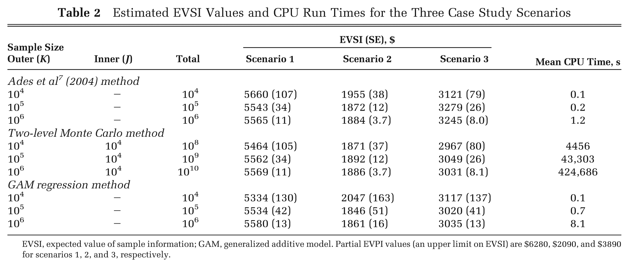
EVSI, expected value of sample information; GAM, generalized additive model. Partial EVPI values (an upper limit on EVSI) are $6280, $2090, and $3890 for scenarios 1, 2, and 3, respectively.

There is good agreement between all 3 methods in scenarios 1 and 2. In scenario 3, the most precise EVSI estimates obtained using the MCMC and GAM methods are in agreement with each other and are approximately $200 lower than the most precise estimate obtained using the Ades et al. ⁷ method.

The analytic method for computing the inner conditional expectation ${\mathbb{E}}_{\mathbf{\theta }|\mathbf{x}}\{\mathrm{NB}(d,\mathbf{\theta })\}$ is exact for scenario 1 but not for scenarios 2 and 3. In scenarios 2 and 3, a Taylor series approximation is used to derive the expectation of a logit-transformed parameter from the expectation of the parameter itself, and in scenario 3, the log odds ratio obtained for each simulated study is assumed to be Normally distributed. These approximations are not required in either the 2-level method or the regression method. The assumption in the analytic method that the study log odds ratios are Normally distributed may in particular be problematic. The assumption is reasonable if the underlying probabilities are close to 0.5 but not when probabilities are close to 0 or 1. In our case study, the mean probability of a critical event is $\mathbb{E}(P_T)=0.044$ on the new treatment and $\mathbb{E}(P_C)=0.15$ on standard care. To explore the robustness of the assumption of Normality, we generated samples from X_T ~ Binom(0.044, 200) and X_C ~ Binom(0.15, 200) and, for each pair of samples, calculated the log odds ratio. A Normal QQ plot of the sampled log odds ratios in Figure 3 shows that the assumption of Normality does not hold.

Figure 3

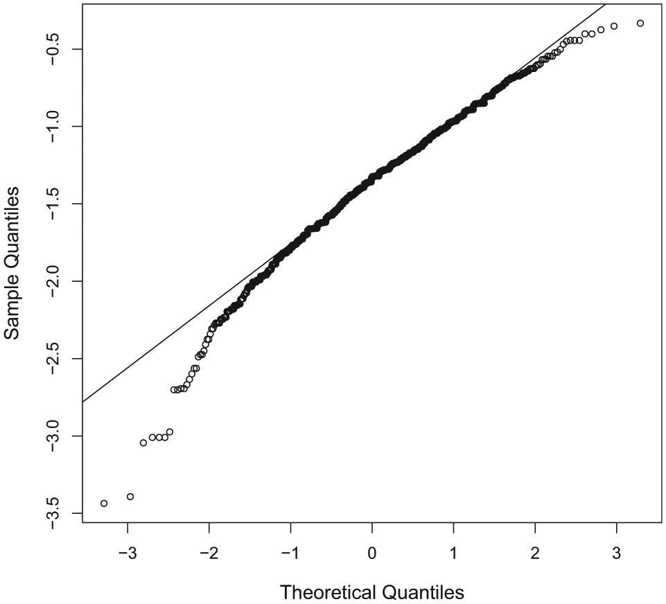
Normal QQ plot for samples of a study log odds ratio with P_T = 0:044, P_C = 0:15, and n_T = n_C = 200.

Precision and Computational Efficiency

For comparisons within each method, the Monte Carlo standard error scales in proportion to K^−1/2 (as expected), and the computation time scales approximately in proportion to K.

For the same level of precision, the 2-level Monte Carlo method requires 10⁴ (i.e., the inner loop size) times as many samples as does the Ades et al. ⁷ analytic method. This holds across all 3 scenarios. The 2-level method is roughly 5 orders of magnitude slower than the Ades et al. method for the same value of K, primarily due to the requirement for 10⁴ model evaluations at each outer-loop run.

For scenario 1, the standard errors obtained using the GAM method are approximately 20% larger than those of the analytic method, given the same number of model runs. Thus, to achieve the same precision, the number of runs would need to be increased by approximately 1.2² = 1.44 times (this was confirmed empirically; results not shown). For scenario 2, the standard errors obtained using the GAM method are approximately 4 times larger than those of the analytic method, given the same number of model runs. Thus, to achieve the same precision, the number of runs would need to be increased by approximately 16 times. For scenario 3, the standard errors obtained using the GAM method are approximately 60% larger than those of the analytic method, given the same number of model runs. Here, to achieve the same precision, the number of runs would need to be increased by approximately 2.6 times.

The precision of the GAM estimate, as well as being related to the sample size, is related to the uncertainty in the model parameters that are not updated by the data. This uncertainty propagates through to the model output (the net benefit) in the PSA sample and causes the variability in the net benefit that is modeled by the error term in the regression. In the case of scenario 2, the GAM estimate requires relatively more samples (for some given precision) than does the GAM estimate for scenario 1 or 3. This suggests that in scenario 2, the uncertainty in the parameters not updated by data (i.e., P_SE and log(OR)) is large. This is confirmed by the relatively high partial EVPI values for P_SE and log(OR).

In terms of computational speed, the GAM method is roughly an order of magnitude slower than the analytic method but roughly 4 orders faster than the 2-level method.

Discussion

Our key idea is that instead of estimating, for each decision option, the posterior expected net benefits via a computationally burdensome repeated (inner-loop) Monte Carlo step, we estimate the functional relationship between the posterior expected net benefit and the simulated data via a nonparametric regression.

Strengths and Limitations

The value of the nonparametric regression method over the 2-level Monte Carlo approach is 2-fold: it is straightforward to implement, requiring less detailed mathematical thinking on the part of the analyst for any particular application, and is several orders of magnitude faster for any given precision. Due to the method’s ease of use and the fact that it only requires the PSA sample and not the model itself, we would suggest that the regression method is applicable in even the simplest of modeling contexts.

In common with other established methods for computing EVSI, we must be able to generate sample data sets, conditional on samples from the prior distribution of the model parameters. For complex study designs, this may not be straightforward. For our method, we must also be able to summarize the sampled data in either a scalar, or low-dimensional, summary statistic. Again, for complex study designs, this may not always be easy.

How This Fits with Existing Literature

One option for computing EVSI is to assume that the incremental net benefit is Normally distributed with parameters that are known functions of study sample size. Under this assumption, EVSI can be calculated using fast analytical methods. This “parametric” approach is most appropriate in settings in which cost-effectiveness analysis is undertaken alongside a single 2-arm randomized controlled trial (RCT). In this setting, the mean incremental net benefit is derived directly from individual-level costs and effects, and the central limit theorem can be used to justify the assumption of Normality. The method has been explored in theoretical investigations^9–13 and applied in real clinical decision problems. ³⁰ However, the approach is not straightforward for decision problems with more than 2 options and may not be appropriate when a more complex decision-analytic model has been used to estimate incremental net benefit. A nonlinear cost-effectiveness model with non-Normal input parameters may generate notably non-Normal incremental net benefits. It may be difficult to predict the relationship between the size of a proposed study that informs some particular subset of parameters and the net benefits of a range of competing decision options. Deriving the parameters of the Normal distribution(s) that the parametric approach requires may therefore be difficult.

The nonparametric regression approach that we propose has some similarities to the model emulation method proposed in Oakley, ³¹ and in one sense, the GAM model can be viewed as an emulator for the posterior expectation of the net benefit, conditional on the data. The important difference between the 2 approaches is that in Oakley, the net benefit function itself is emulated. Emulating the net benefit function allows for the rapid evaluation of a slow economic model, but it does not address the problem of how to sample from a difficult posterior distribution of the parameters conditional on the data. Our method also has some similarities to the spline-based approach for computing partial EVPI that has been proposed by Madan et al. ²¹ Here, a spline is used to approximate the conditional expectation of some predefined subfunction of the net benefit function, given some sampled value of a parameter of interest. Although the method by Madan et al is shown to perform well, it requires algebraic manipulation of the net benefit function to identify the appropriate subfunctions for the spline approximation. This may be difficult in complex models.

Implications for Practice and for Research

At present, commissioners and funders of research are not using EVSI methods as part of their day-to-day decision-making processes (although there are exceptions to this^30,32,33). However, it is becoming more common for early economic evaluation models to be requested by research funders to establish the potential benefits of proposed new interventions. One barrier to implementation of EVSI at this stage has been the complexity of calculation, and we hope that our method can help to remove this barrier. We do recognize, though, that there are other important barriers to the widespread use of EVSI, including a lack of understanding of value of information methods, a mistrust of mathematical models, and a requirement for trialists to work within a frequentist hypothesis test-based framework.

Throughout the article, we have assumed that the decision maker’s utility is equal to net benefit and that the decision problem is to maximize net benefit over a set of discrete treatment options. This is the typical decision problem faced by government agencies such as the National Institute for Health and Care Excellence (NICE), but the type of decision problem faced by the pharmaceutical industry is somewhat different. Here, utility is profit, and under value-based pricing, the decision problem is to choose price to maximize profit, subject to the constraint that additional health benefits do not cost more than the funder’s willingness to pay. EVSI from an industry perspective has been explored by Willan ³⁴ and by Willan and Eckermann, ³⁵ as well as more recently within a value-based pricing context by Breeze and Brennan. ³⁶ Our nonparametric regression method for computing EVSI will apply equally well in this context.

Further research could extend to testing the nonparametric regression method in other cost-effectiveness models, including Markov cohort models and more complex patient-level models. An important feature of our method is that all variation in the net benefit function that is not due to the data is taken up by the error term in the regression analysis and “averaged out.” Thus, any variation in the net benefit that arises due to poor convergence of a patient-level model is also averaged out in the regression. ²⁴ This means that, to calculate EVSI for a patient-level model (in which patients do not interact), only a single patient needs to be “run” through the model at each evaluation of the PSA. We look forward to more research in this area.