An Efficient Method for Computing Single-Parameter Partial Expected Value of Perfect Information

Abstract

The value of learning an uncertain input in a decision model can be quantified by its partial expected value of perfect information (EVPI). This is commonly estimated via a 2-level nested Monte Carlo procedure in which the parameter of interest is sampled in an outer loop, and then conditional on this sampled value, the remaining parameters are sampled in an inner loop. This 2-level method can be difficult to implement if the joint distribution of the inner-loop parameters conditional on the parameter of interest is not easy to sample from. We present a simple alternative 1-level method for calculating partial EVPI for a single parameter that avoids the need to sample directly from the potentially problematic conditional distributions. We derive the sampling distribution of our estimator and show in a case study that it is both statistically and computationally more efficient than the 2-level method.

The value of learning an input to a decision-analytic model can be quantified by its partial expected value of perfect information (partial EVPI). ^{1 –4} The partial expected value of information for some model input, X_i , is the expected difference between the value of the optimal decision based on perfect information about X_i and the value of the decision made only with prior information. To express this formally, we first introduce some notation.

We assume that we are faced with D decision options, indexed d = 1, . . ., D, and have built a model y_d = f (d, x) that aims to predict the net benefit of decision option d given a vector of input parameter values x. We denote the true unknown values of the inputs X = {X ₁,. . .,X_p }, and the uncertain net benefit under decision option d as Y_d . We denote the input parameter for which we wish to calculate the partial EVPI as X_i and the remaining input parameters as ${\mathbf{X}}_{-i}=\{X_1,\dots ,{\mathbf{X}}_{i-1},X_{i+1},\dots ,X_p\}$ . We denote the expectation over the full joint distribution of X as E_X , over the marginal distribution of X_i as $E_{X_i}$ , and over the conditional distribution of ${\mathbf{X}}_{-i}|X_i$ as $E_{{\mathbf{X}}_{-i}|X_i}$ .

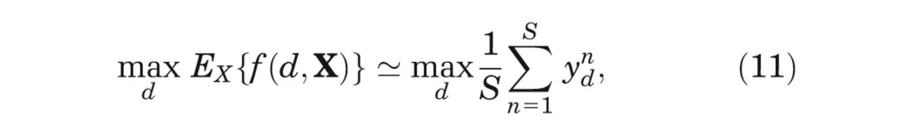
The expected value of our optimal decision, made only with current information, is

$$\underset{d}{max}{E}_X\{f(d,\mathbf{X})\}.$$

If we knew the value of some input of interest, X_i , then the optimal decision would be that with the greatest net benefit, after averaging over the conditional distribution of the remaining unknown inputs, ${\mathbf{X}}_{-i}|X_i$ . The expected net benefit would be

$$\underset{d}{max}{E}_{{\mathbf{X}}_{-i}|X_i}\{f(d,X_i,{\mathbf{X}}_{-i})\}.$$

But, since X_i is unknown, we must average over our current information about X_i , giving

$$E_{X_i}\left[\underset{d}{max}{E}_{{\mathbf{X}}_{-i}|X_i}\{f(d,X_i,{\mathbf{X}}_{-i})\}\right].$$

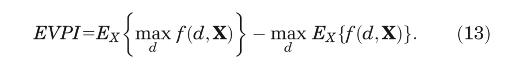
The partial EVPI for input X_i is the difference between equation (3), the expected value of the decision made with perfect information about X_i , and equation (1), the expected value of the current optimal decision option, ^3,4

$$EVPI(X_i)=E_{X_i}\left[\underset{d}{\max }{E}_{{\mathbf{X}}_{-i}|X_i}\left\{f(d,X_i,{\mathbf{X}}_{-i})\right\}\right]-\underset{d}{\max }{E}_X\{f(d,\mathbf{X})\}.$$

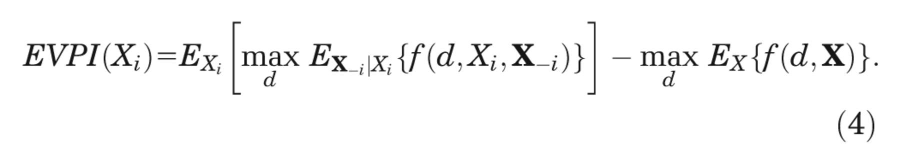
We are commonly in a situation in which we cannot evaluate any of the 3 expectations in equation (4) analytically. Important exceptions are cases in which models are either of linear form (e.g., $Y_1={\beta }_1{X}_1+{\beta }_2{X}_2$ ) or multilinear (sum-product) form (e.g., $Y_1={\beta }_1{X}_1{X}_2+{\beta }_2{X}_3{X}_4$ ) (where β₁ and β₂ are constants). In the linear case, the expectation in equation (1) and the inner expectation in equation (3) both have an analytic solution, and in the multilinear case, these expectations have an analytic solution if inputs are independent. In the case of correlated inputs, analytic solutions to these 2 expectations will sometimes exist, such as the case in which the inputs have a multivariate Normal distribution. The outer expectation in equation (3) is more problematic due to the maximization step, and analytic solutions rarely exist.

In the absence of analytic solutions to the expectations in equation (3), the usual approach is to use a nested 2-level Monte Carlo method. This requires us to sample a value of the input parameter of interest in an outer loop and then to sample values from the joint conditional distribution of the remaining parameters and run the model in an inner loop. ^5,6 Sufficient numbers of runs of both the outer and inner loops are required to ensure that the partial EVPI is estimated with sufficient precision and with an acceptable level of bias. ⁷

We recognize 2 important practical limitations to the standard 2-level Monte Carlo approach to calculating partial EVPI. First, the nested 2-level nature of the algorithm with a model run at each inner-loop step can be highly computationally demanding for all but very small loop sizes if the model is expensive to run. Second, we require a method of sampling from the joint distribution of the inputs (excluding the parameter of interest) conditional on the input parameter of interest. If the input parameter of interest is independent of the remaining parameters, then we can simply sample from the unconditional joint distribution of the remaining parameters. However, if inputs are not independent, we may need to resort to Markov chain Monte Carlo (MCMC) methods if there is no analytic solution to the joint conditional distribution. Including an additional MCMC step in the algorithm is likely to increase the computational burden considerably, as well as requiring additional programming.

In this article, we present a simple 1-level “ordered input” algorithm for calculating single-parameter partial EVPI, which requires only a single set of the sampled inputs and corresponding outputs to calculate partial EVPI values for all input parameters. The method is applicable in any modeling scenario in which there is no analytic solution to the expectations in equation (4). The method avoids the nested double loop and is therefore computationally less demanding than the standard 2-level method, and it also avoids the need to sample directly from the conditional distributions of the inputs when inputs are correlated. We describe methods for quantifying the upward bias and precision of the estimator. We illustrate the method in a case study with 2 scenarios: a multilinear model in which inputs are correlated, but with known analytic solutions for all conditional distributions, and the same model in which inputs are correlated but where sampling from the conditional distributions requires MCMC.

Methods

In this section, we describe an algorithm for computing the partial EVPI for a single input parameter of interest, X_i . Code for implementing the algorithm in R ⁸ is shown in Appendix A and is available for download at http://www.shef.ac.uk/scharr/sections/ph/staff/profiles/mark.

Briefly, the idea is as follows. We assume we have a set of samples from the joint distribution of the model input parameters and a corresponding set of model outputs (i.e., net benefits). The net benefits (for each decision option) are ordered with respect to the input of interest and then partitioned into subsets of equal size. Within each subset, we calculate the mean of the net benefits for each decision option and take the maximum across the decision options. The average of these maxima is taken as an approximation to the first term in equation (4). The second term in equation (4) is computed using standard Monte Carlo sampling—that is, for each decision option, we calculate the mean of the net benefits corresponding to the whole set of input samples and then take the maximum of these means.

In the following subsections, we introduce notation and describe the algorithm in detail in a series of stages.

Stage 1

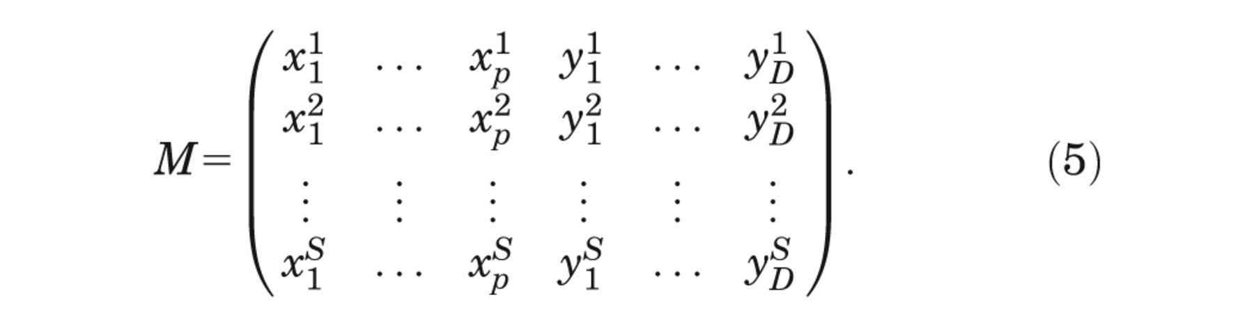
We define the Monte Carlo sample of model inputs and corresponding model outputs as $\{(x^s,y_d^s),s=1,\dots ,S,d=1,\dots ,D\}$ , where the x ^s are drawn from the joint distribution of the inputs, p(X), and $y_d^s=f(d,x^s)$ is the evaluation of the model output at x ^s for decision option d. Note the use of superscripts to index the randomly drawn sample sets. We let M be the matrix of inputs and corresponding outputs

$$M=\left(\begin{array}{cccccc}{x}_1^1& \dots & x_p^1& y_1^1& \dots & y_D^1\\ x_1^2& \dots & x_p^2& y_1^2& \dots & y_D^2\\ ⋮& ⋮& ⋮& ⋮& ⋮& ⋮\\ x_1^S& \dots & x_p^S& y_1^S& \dots & y_D^S\end{array}\right).$$

Stage 2

For parameter of interest i, we extract the x_i and y ₁,. . . ,y_D columns and reorder with respect to x_i , giving

$$M^{*}=\left(\begin{array}{cccc}{x}_i^{(1)}& y_1^{(1)}& \dots & y_D^{(1)}\\ x_i^{(2)}& y_1^{(2)}& \dots & y_D^{(2)}\\ ⋮& ⋮& ⋮& ⋮\\ x_i^{(S)}& y_1^{(S)}& \dots & y_D^{(S)}\end{array}\right),$$

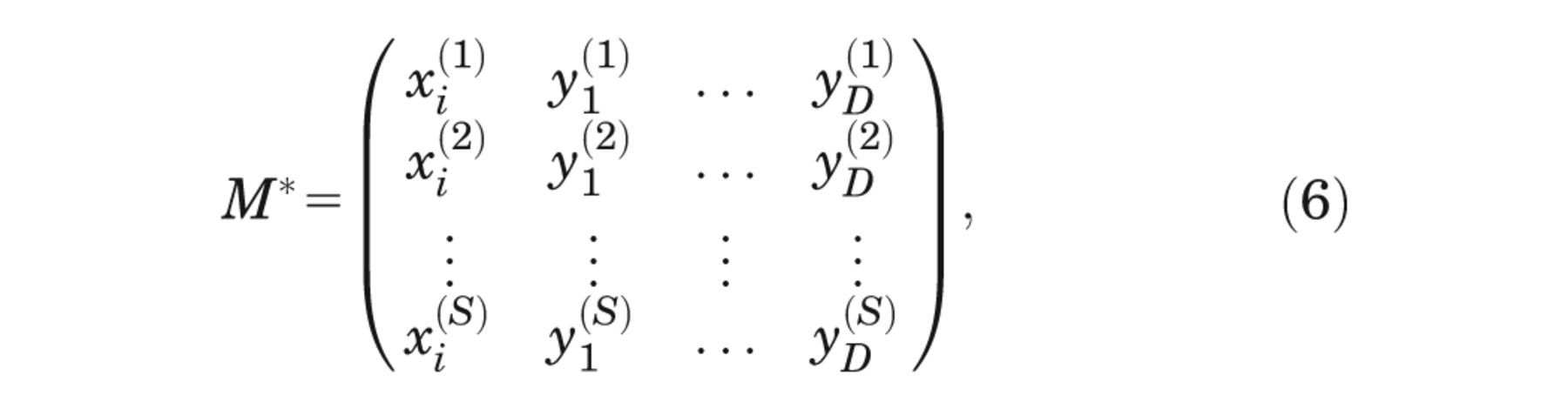
where $x_i^{(1)}\le x_i^{(2)}\le \dots \le x_i^{(S)}$ . Note the use of bracketed superscripts to denote the sample set ordered with respect to the input of interest.

Stage 3

We partition the resulting matrix into k = 1,. . .,K submatrices $M^{*(k)}$ of J rows each,

$$M^{*(k)}=\left(\begin{array}{cccc}{x}_i^{(1,k)}& y_1^{(1,k)}& \dots & y_D^{(1,k)}\\ x_i^{(2,k)}& y_1^{(2,k)}& \dots & y_D^{(2,k)}\\ ⋮& ⋮& ⋮& ⋮\\ x_i^{(J,k)}& y_1^{(J,k)}& \dots & y_D^{(J,k)}\end{array}\right),$$

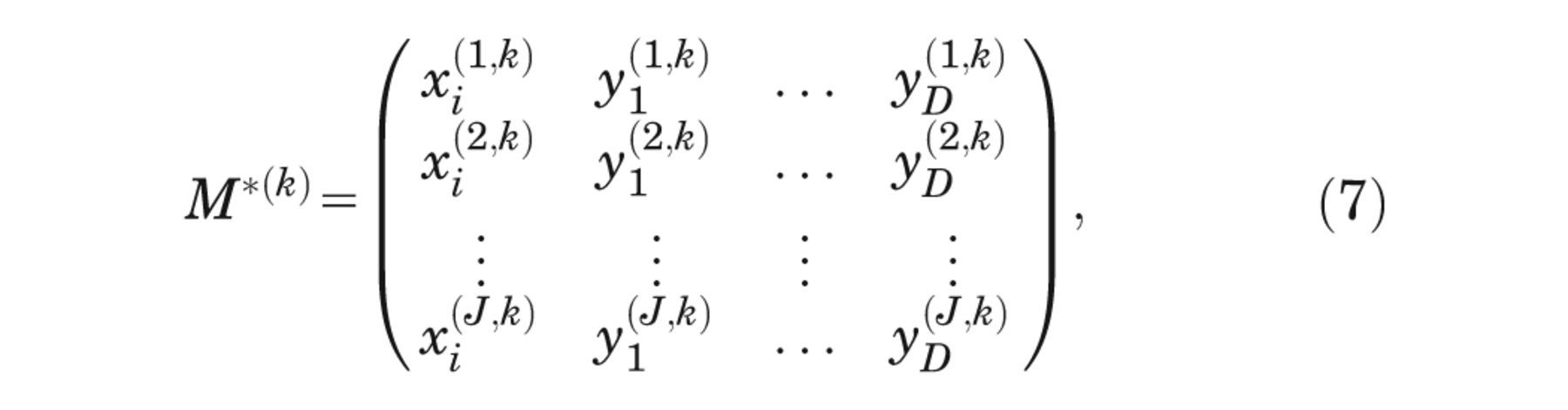
retaining the ordering with respect to x_i , and where the row indexed (j, k) in equation (7) is the row indexed (j + (k − 1)J) in equation (6). Note that J × K must equal the total sample size S.

Stage 4

For each $M^{*(k)}$ , we estimate (for each decision option) the conditional expectation ${\mu }_d^{(k)}=E_{{\mathbf{X}}_{-i}|{\mathbf{X}}_i=x_i^{*(k)}}\{f(d,X_i,{\mathbf{X}}_{-i})\}$ by averaging over j = 1, . . . , J, that is,

$$\begin{array}{c}{\hat{\mu }}_d^{(k)}=\frac{1}{J}\sum _{j=1}^J{y}_d^{(j,k)},\end{array}$$

where $x_i^{*(k)}=\sum _{j=1}^J{x}_i^{(j,k)}/J$ .

The justification for this rests on recognizing that if J is small compared with S, then the ordered values of the input of interest $\{x_i^{(1,k)},\dots ,x_i^{(J,k)}\}$ will all be close to their mean value, $x_i^{*(k)}$ , and the corresponding values of the remaining inputs $\{x_{-i}^{(1,k)},\dots ,x_{-i}^{(J,k)}\}$ will be (approximately) a sample from the distribution of ${\mathbf{X}}_{-i}|X_i=x_i^{*(k)}$ . See Appendix B for a more formal justification.

The maximum $m^{(k)}=\underset{d}{max}{E}_{{\mathbf{X}}_{-i}|X_i=x_i^{*(k)}}\{f(d,X_i,{\mathbf{X}}_{-i})\}$ is then estimated by

$$\begin{array}{c}{\hat{m}}^{(k)}=\underset{d}{max}{\hat{\mu }}_d^{(k)},\end{array}$$

and finally we estimate the first term on the right-hand side of equation (4) by averaging over k = 1, . . . ,K, that is,

$$\overline{\hat{m}}=\frac{1}{K}\sum _{k=1}^K{\hat{m}}^{(k)}.$$

Stage 5

We estimate the second term on the right-hand side of equation (4) using simple Monte Carlo sampling, that is,

$$\underset{d}{max}{E}_X\{f(d,\mathbf{X})\}\approx \underset{d}{max}\frac{1}{S}\sum _{n=1}^S{y}_d^n,$$

where the order of the xⁿ is irrelevant.

Stages 2 to 4 are repeated for each parameter of interest, noting that only a single set of model runs (stage 1) is required.

Choosing Values For J And K

We assume that we have a fixed number of model evaluations S and wish to choose values for J and K subject to the constraint J × K = S.

First, we note that for small values of J, the EVPI estimator is upwardly biased due to the maximization in equation (9). ⁷ Indeed, for J = 1 (and K = S), our ordered input estimator for the first term on the right-hand side of equation (4) reduces to

$$\frac{1}{S}\sum _{s=1}^S\underset{d}{max}(y_d^s),$$

which is the Monte Carlo estimator for the first term in the expression for the overall EVPI,

$$\mathrm{EVPI}=E_X\{\underset{d}{max}f(d,\mathbf{X})\}-\underset{d}{max}{E}_X\{f(d,\mathbf{X})\}.$$

Second, we note that for very large values of J, and hence small values of K, the EVPI estimator is downwardly biased and converges to zero when J = S. In this case, our ordered input estimator for the first term on the right-hand side of equation (4) reduces to

$$\underset{d}{max}\frac{1}{S}\sum _{s=1}^S{y}_d^s,$$

which is the Monte Carlo estimator for the second term on the right-hand side of Equation 4.

The precision of the partial EVPI estimate only depends on S and not on J and K (see Appendix C for the derivation of an expression for the variance of the estimator). We therefore only need to consider the minimization of bias in our choice of J and K when S is fixed. Because the upward bias due to small J converges to zero as J increases, a sensible choice of J is that which is just large enough such that the estimated bias $\hat{b}$ is smaller than some constant c. Any choice of J larger than this will risk introducing a downward bias that becomes apparent at small values of K.

We estimate the upward bias in the following manner, using the method proposed by Oakley and others. ⁷ First, we write the vector of Monte Carlo estimators for the conditional expected net benefits from equation (8) as ${\hat{\mu }}^{(k)}={({\hat{\mu }}_1^{(k)},\dots ,{\hat{\mu }}_D^{(k)})}^{\prime }$ . If we can determine the sampling distribution of this vector of estimators, then we can quantify the upward bias in $\overline{\hat{m}}$ and hence the upward bias in the partial EVPI.

Unless J is very small, ${\hat{\mu }}^{(k)}$ will follow a multivariate Normal distribution with D dimensions. Thus, we have

$${\hat{\mu }}^{(k)}~N_D({\mu }^{(k)},\frac{1}{J}{\mathbf{V}}^{(k)}),$$

where ${\mathbf{\mu }}^{(k)}={({\mu }_1^{(k)},\dots ,{\mu }_D^{(k)})}^{\prime }$ , and where each element p,q of ${\mathbf{V}}^{(k)}$ is estimated by

$${\hat{V}}_{p,q}^{(k)}=\text{cov}({\hat{\mu }}_p^{(k)},{\hat{\mu }}_q^{(k)}).$$

To estimate the bias in $\overline{\hat{m}}$ , we first draw, for each k = 1, . . . , K, a set of N samples from a multivariate Normal distribution with mean vector ${\hat{\mu }}^{(k)}$ and variance matrix $\frac{1}{J}{\hat{V}}_{p,q}^{(k)}$ . We choose N to be large, say 1000. Let us denote these samples ${\tilde{\mu }}_n^{(k)}=({\tilde{\mu }}_{1,n}^{(k)},\dots ,{\tilde{\mu }}_{D,n}^{(k)})$ for n = 1, . . . , N and k = 1, . . . , K. The bias in ${\hat{m}}^{(k)}$ is estimated by

$${\hat{b}}^{(k)}=\frac{1}{N}\sum _{n=1}^{N}max\{{\tilde{\mu }}_{1,n}^{(k)},\dots ,{\tilde{\mu }}_{D,n}^{(k)}\}-max\{{\hat{\mu }}_1^{(k)},\dots ,{\hat{\mu }}_D^{(k)}\},$$

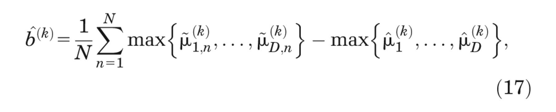
and the expected bias in $\overline{\hat{m}}$ as

$$\hat{b}=\frac{1}{K}\sum _{k=1}^K{\hat{b}}^{(k)}.$$

R code for computing the bias estimate is available for download at http://www.shef.ac.uk/scharr/sections/ph/staff/profiles/mark.

The left panel of Figure 1 shows $\hat{b}$ , the expected upward bias in the partial EVPI for various values of J (on the log₁₀ scale) for input X ₆ in the first scenario of the case study outlined later in the article. The total number of model evaluations, S, is 1,000,000, and K = S/J. Note the convergence to zero as J increases. The arrow is placed at J = 1000, the smallest value of J for which the bias is less than £1.

Figure 1

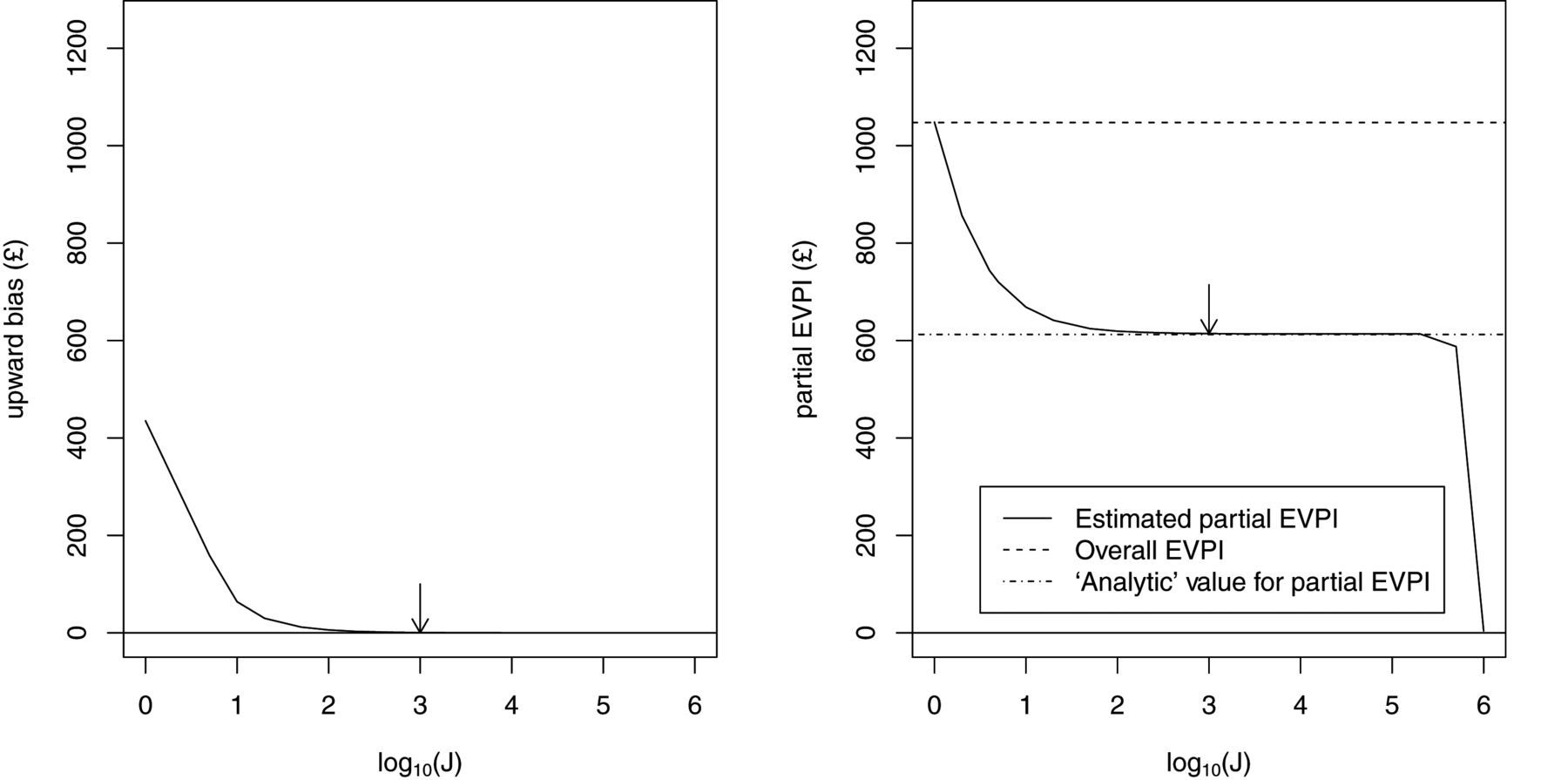
Left panel: upwards bias in partial expected value of perfect information (EVPI) estimator against log₁₀ (J). Right panel: estimated partial EVPI at values of J ranging from 1 to 10⁶ where the total number of model evaluations, S, is 10⁶ . The arrows show the smallest value of J for which the bias is less than £1 (J = 1000 in this case).

The right panel shows values for the estimated partial EVPI against J (on the log₁₀ scale). In scenario 1 of the case study, the inner expectation of equation (4) has an analytic solution, and we were therefore able to compute a value of the partial EVPI values for all parameters to high precision using a simple 1-level Monte Carlo sampling scheme. This “analytic” value is shown in the figure, as is the overall EVPI for all parameters. The total number of model evaluations S is again 1,000,000, with K = S/J. Note the upward and downward biases at extreme values of J but also the large region of stability between J = 100 (K = 10, 000) and K = 100, 000 (K = 10). The arrow is placed at J = 1000, the smallest value of J for which the bias is less than £1. At this point, the estimated partial EVPI is £612.63 compared with the analytic value of £612.38.

Case Study

The case study is based on a hypothetical decision tree model previously used for illustrative purposes in Brennan and others, ⁵ Oakley and others, ⁷ and Kharroubi and others. ⁹ The model predicts monetary net benefit, Y_d , under 2 decision options (d = 1, 2) and can be written in sum product form as

$$Y_1=\lambda (X_5{X}_6{X}_7+X_8{X}_9{X}_{10})-(X_1+X_2{X}_3{X}_4),$$

$$Y_2=\lambda (X_{14}{X}_{15}{X}_{16}+X_{17}{X}_{18}{X}_{19})-(X_{11}+X_{12}{X}_{13}{X}_4),$$

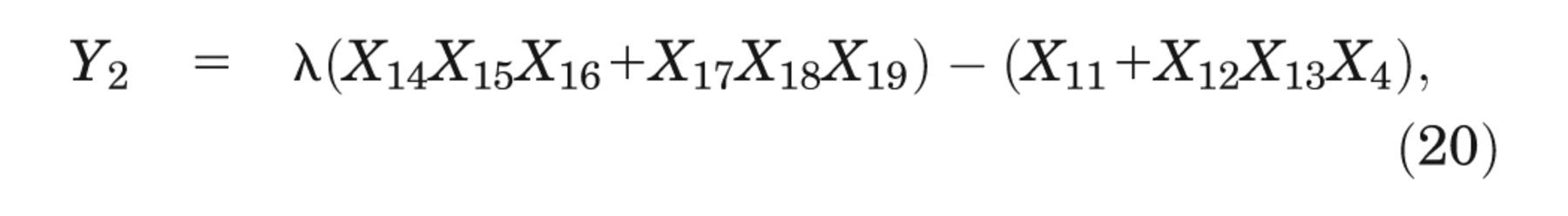
where $\mathbf{X}=\{X_1,\dots ,X_{19}\}$ are the 19 uncertain input parameters listed in Table 1, and the willingness to pay for 1 unit of health output in quality-adjusted life years (QALYs) is λ = £10,000/QALY.

Table 1

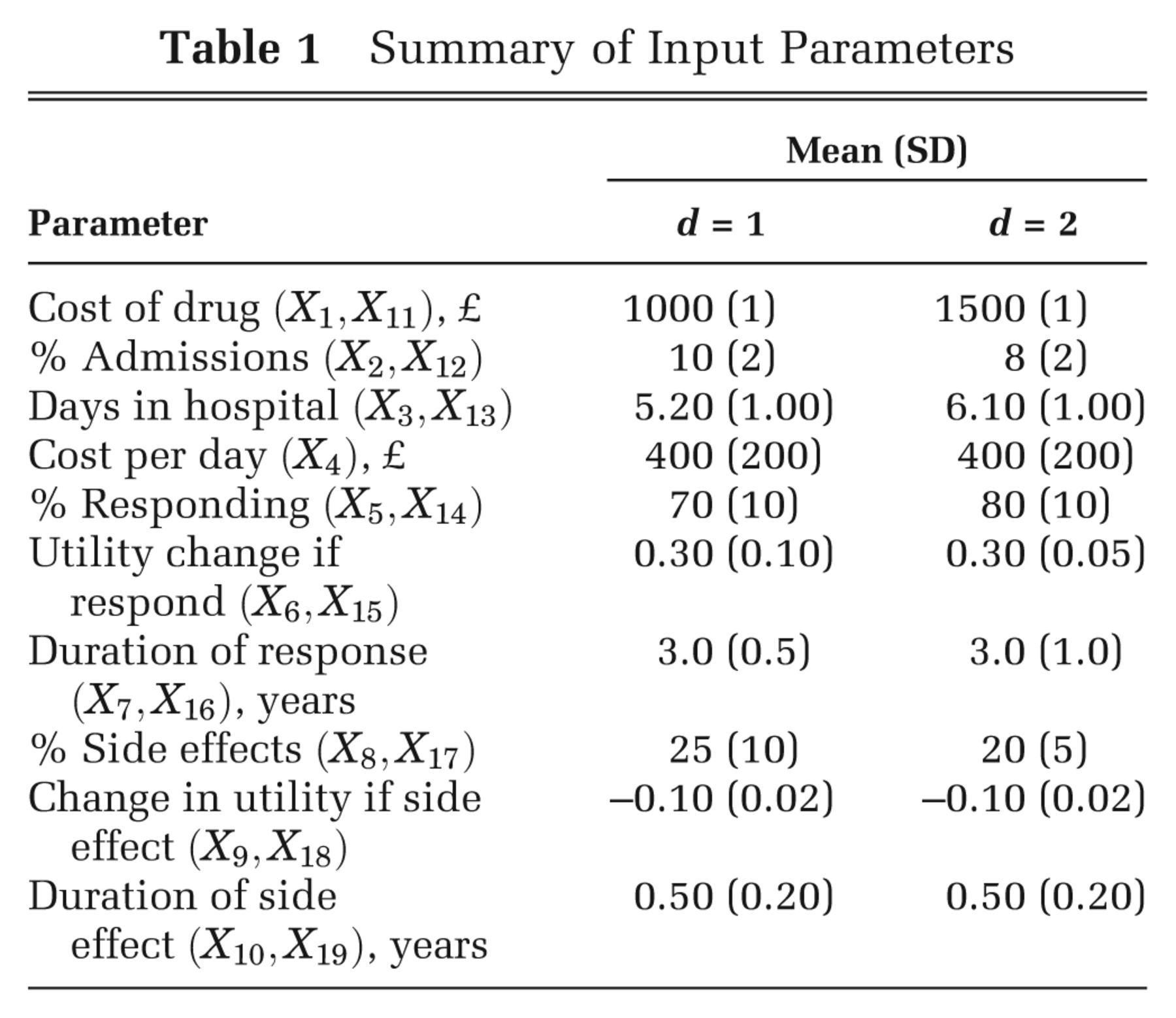
Summary of Input Parameters

	Mean (SD)
Parameter	d = 1	d = 2
Cost of drug (X 1, X 11), £	1000 (1)	1500 (1)
% Admissions (X 2, X 12)	10 (2)	8 (2)
Days in hospital (X 3, X 13)	5.20 (1.00)	6.10 (1.00)
Cost per day (X 4), £	400 (200)	400 (200)
% Responding (X 5, X 14)	70 (10)	80 (10)
Utility change if respond (X 6, X 15)	0.30 (0.10)	0.30 (0.05)
Duration of response (X 7, X 16), years	3.0 (0.5)	3.0 (1.0)
% Side effects (X 8, X 17)	25 (10)	20 (5)
Change in utility if side effect (X 9, X 18)	−0.10 (0.02)	−0.10 (0.02)
Duration of side effect (X 10, X 19), years	0.50 (0.20)	0.50 (0.20)

Scenario 1: Correlated Inputs with Known Conditional Distributions

In scenario 1, we assume that a subset of the inputs are correlated but with a joint distribution such that we can sample from the conditional distributions of the correlated inputs without the need for MCMC. We assume that the inputs are jointly Normally distributed, with X ₅, X ₇, X ₁₄, and X ₁₆ all pairwise correlated with a correlation coefficient of 0.6 and with all other inputs independent. In a simple sum product form model, the assumption of multivariate Normality allows us to compute the inner conditional expectation analytically, as well as allowing us to sample directly from the conditional distribution ${\mathbf{X}}_{-i}|X_i$ in the standard nested 2-level method, but this will not necessarily be the case in models with additional nonlinearity.

We calculated partial EVPI using 3 methods. First, we calculated the partial EVPI for each parameter using a single-loop Monte Carlo approximation for the outer expectation in the first term of the right-hand side of equation (4) with 10⁶ samples from the distribution of the parameter of interest, as well as an analytic solution to the inner conditional expectation. Next, we calculated the partial EVPI values using the standard 2-level Monte Carlo approach with 1000 inner-loop samples and 1000 outer-loop samples (i.e., 1000 × 1000 = 10⁶ model evaluations in total). Finally, we computed the partial EVPI values using the ordered sample method with the same number of model evaluations, S = 10⁶, and values of J = K = 1000.

Standard errors and bias estimates for the 2-level Monte Carlo partial EVPI estimates were obtained using the methods presented in Oakley and others. ⁷ The standard errors for the ordered input method partial EVPI estimates were obtained using the method presented in Appendix C. The bias estimates for the ordered input method partial EVPI estimates were obtained using the method presented in the Methods section above. We measured the total computation time for obtaining EVPI values for all 19 parameters.

Results for Scenario 1

Calculating the expected net benefits for decision options 1 and 2 analytically results in values of £5057.00 and £5584.80, respectively, indicating that decision option 2 is optimal. Running the model with 10⁶ Monte Carlo samples from the joint distribution of the input parameters results in option 2 having greater net benefit than option 1 in only 54% of samples, suggesting that the input uncertainty is resulting in considerable decision uncertainty. The overall EVPI is £1046.10.

The partial EVPI values for parameters X ₁ to X ₄, X ₈ to X ₁₃, and X ₁₇ to X ₁₉ were all less than £0.01 and therefore considered unimportant in terms of driving the decision uncertainty. Results for the remaining parameters are shown in Table 2. The standard errors of the partial EVPI values estimated via the ordered input method are considerably smaller than those estimated via the 2-level method, whereas the estimated bias for each parameter is similar. The ordered input method is approximately 4 times faster than the standard 2-level Monte Carlo method in this case.

Table 2

Partial Expected Value of Perfect Information (EVPI) Values for Scenario 1

	Partial EVPI (SE; Estimated Bias), £
Parameter	Analytic Conditional Expectation	Two-Level Monte Carlo	Ordered Input Method
X 5	22.50	9.52 (65.20; 1.85)	25.29 (3.26; 1.62)
X 6	612.38	614.76 (33.02; 0.46)	612.63 (3.15; 0.50)
X 7	11.56	77.65 (66.38; 1.31)	14.86 (3.28; 1.61)
X 14	230.94	312.39 (69.59; 1.55)	233.63 (3.19; 1.42)
X 15	271.52	315.02 (29.52; 1.45)	273.00 (3.30; 1.17)
X 16	458.97	502.91 (77.98; 0.85)	462.42 (3.12; 0.65)
Computation time a		4.2	1

a

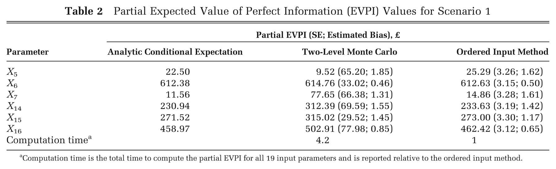
Computation time is the total time to compute the partial EVPI for all 19 input parameters and is reported relative to the ordered input method.

Scenario 2: Correlated Inputs with Conditional Distribution Sampling Requiring MCMC

In scenario 2, we assume that a subset of the inputs are correlated but with a joint distribution such that we can only sample from the conditional distributions of the correlated inputs using MCMC. We assume, as in scenario 1, that X ₅, X ₇, X ₁₄, and X ₁₆ are pairwise correlated, but with a more complicated dependency structure based on an unobserved bivariate Normal latent variable $\mathbf{Z}=(Z_1,Z_2)$ that has expectation zero, variance 1, and correlation 0.6. Conditional on this latent variable, which represents some measure of effectiveness, the proportions of responders (X ₅ and X ₁₄) are assumed beta distributed and the durations of response (X ₇ and X ₁₆) assumed gamma distributed. The hyperparameters of the beta and gamma distributions are defined in terms of Z such that X ₅, X ₇, X ₁₄, and X ₁₆ have the means and standard deviations in Table 1.

We calculated partial EVPI for each parameter using the standard 2-level Monte Carlo approach with 1000 inner-loop samples and 1000 outer-loop samples (i.e., 1000 × 1000 = 10⁶ model evaluations in total) using OpenBUGS ¹⁰ to sample from the conditional distribution of ${\mathbf{X}}_{-i}|X_i$ . Finally, we computed the partial EVPI values using the ordered sample method with the same number of model evaluations, S = 10⁶, and values of J = K = 1000.

Results for Scenario 2

Running the model with 10⁶ samples from the joint distribution of the input parameters resulted in expected net benefits of £5043.12 and £5549.93 for decision options 1 and 2, respectively, indicating that decision option 2 is optimal, but again with considerable decision uncertainty. Based on this sample, the probability that decision 2 is best is 54%, and the overall EVPI is £1240.33.

Partial EVPI results are shown in Table 3. Values for parameters X ₁ to X ₄, X ₈ to X ₁₃, and X ₁₇ to X ₁₉ were again all less than £0.01 and are not shown. Standards errors for the partial EVPI values estimated via the ordered input method are again smaller than those estimated via the 2-level method. The estimated bias is marginally smaller for the ordered input method. The ordered input method is approximately 800 times faster than the 2-level Monte Carlo/MCMC method in this case.

Table 3

Partial Expected Value of Perfect Information (EVPI) Values for Scenario 2

	Partial EVPI (SE; Bias), £
Parameter	Two-Level Monte Carlo with MCMC Inner Loop	Ordered Input Method
X 5	102.55 (34.48; 3.82)	34.65 (3.26; 0.82)
X 6	610.82 (38.02; 0.93)	618.80 (3.10; 0.78)
X 7	132.16 (36.10; 4.57)	56.25 (3.25; 0.81)
X 14	334.13 (51.94; 1.43)	368.87 (3.18; 0.77)
X 15	223.09 (25.73; 2.04)	275.78 (3.25; 0.82)
X 16	554.20 (64.00; 0.89)	663.25 (3.13; 0.80)
Computation time a	810	1

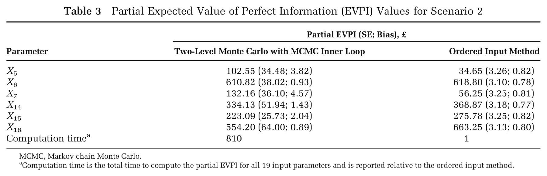
MCMC, Markov chain Monte Carlo.

a

Computation time is the total time to compute the partial EVPI for all 19 input parameters and is reported relative to the ordered input method.

How Many 2-Level Monte Carlo Inner- and Outer-Loop Samples Are Required to Achieve a Bias and Precision Similar to the Ordered Input Method?

We compared the bias and precision of the partial EVPI estimated via the ordered method with that estimated via the 2-level method with a range of inner- and outer-loop sizes. Our comparator was the partial EVPI for input parameter X ₆ for scenario 1 computed using the ordered 1-level method with a total sample size of 10⁶ and J = K = 1000. Using this method, the upward bias was estimated to be £0.50, and the standard error of the estimate was £3.15 (Table 2). Table 4 shows the bias and standard error for the 2-level Monte Carlo method for different inner- and outer-loop sizes, which were estimated using the method proposed by Oakley and others. ⁷ The reported computation times are relative to the time taken for the ordered input method with a sample size of 10⁶ and J = K = 1000.

Table 4

Standard Error and Bias for Parameter X ₆ in Scenario 1, Computed via the 2-level Monte Carlo Method for a Range of Inner- and Outer-Loop Sizes

	SE (Estimated Bias), £
	[Relative Computation Time a ]
	Outer Loop
Inner Loop	10	100	1000	10,000	100,000
10	437.55 (56.93)	138.41(59.27)	43.74 (58.38)	13.84 (57.70)	4.38 (58.73)
	[0.0015]	[0.012]	[0.12]	[1.24]	[12.97]
100	341.82 (5.47)	108.11 (5.82)	34.18 (5.46)	10.81 (5.56)	3.42 (5.61)
	[0.0024]	[0.020]	[0.19]	[1.96]	[20.59]
1000	330.24 (0.52)	104.43 (0.55)	33.02 (0.46)	10.44 (0.67)	3.30 (0.47)
	[0.010]	[0.091]	[0.93]	[9.38]	[99.91]
10,000	329.05 (0.08)	104.05 (0.06)	32.91 (0.02)	10.41 (0.07)	3.29 (0.01)
	[0.095]	[0.84]	[8.08]	[80.92]	[801.53]
100,000	328.93 (0.01)	104.02 (0.01)	32.89 (0.02)	10.40 (0.02)	3.29 (0.01)
	[0.79]	[8.29]	[82.18]	[819.93]	[8139.48]

a

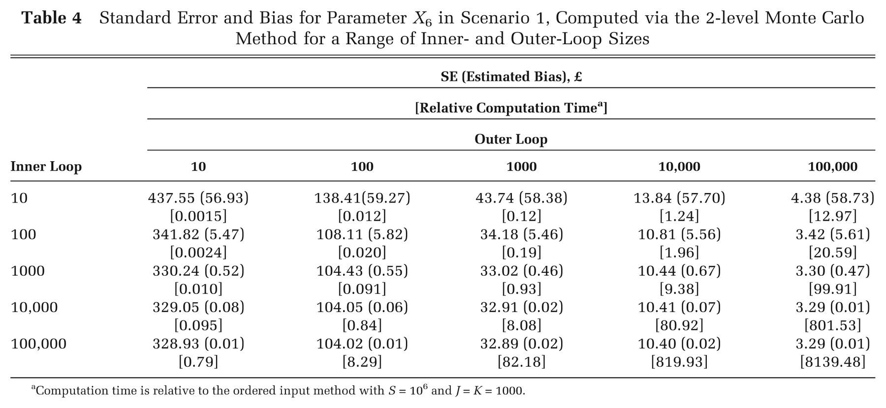
Computation time is relative to the ordered input method with S = 10⁶ and J = K = 1000.

To achieve a similar precision and bias via the 2-level Monte Carlo method, the outer loop must be of the order of 100,000 and the inner loop of the order of 1000. This therefore requires 10⁸ model evaluations and is approximately 100 times slower to compute than the ordered input method.

Discussion

We have presented a method for calculating the partial expected value of perfect information that is simple to implement, is rapid to compute, and does not require an assumption of independence between inputs. The saving in computational time is particularly marked if the alternative is to use a nested 2-level EVPI approach in which the conditional expectations are estimated using MCMC. The method is straightforward to apply in a spreadsheet application, even with little programming knowledge.

Our approach requires only a single set of model evaluations to calculate partial EVPI for all inputs, allowing a complete separation of the EVPI calculation step from the model evaluation step. This separation may be particularly useful when the model has been evaluated using specialist software (e.g., for discrete event or agent-based simulation) that does not allow easy implementation of the EVPI step or when those who wish to compute the EVPI do not “own” (and therefore cannot directly evaluate) the model. The method does require that, if any inputs are correlated, the inputs are sampled from their joint distribution, rather than from their separate marginal distributions. However, this is unlikely to be an important limitation. When inputs are correlated, sampling from their joint distribution is usual practice, for example, when sampling Dirichlet distributed transition probabilities or multivariate Normal distributed regression parameters.

As presented, the method calculates the partial EVPI for single inputs one at a time. We may, however, wish to calculate the value of learning groups of inputs simultaneously. There are good reasons for this. First, for certain forms of model, we may find that learning single inputs alone has little value, but learning a group of inputs has high value due to the interactions between those inputs within the model. It is important to note that interactions result from nonadditive effects within the model and can occur even if inputs are uncorrelated. Second, a certain subset of model inputs may be derived from a single study, and therefore learning one input in this set (by conducting the “perfect” study) implies learning them all. If we are considering the value of a study in reducing uncertainty about inputs, we will consider the value of all the information that arises from the study, not just the information that informs a single input. The value of our method may then be in drilling down to specific inputs or small groups of inputs within some larger group of inputs that is judged to be policy relevant. If inputs can be partitioned into broad policy-relevant groups (i.e., those that might be considered together when a decision is made to commission further research), and if these groups can be treated as uncorrelated, then calculating the EVPI for each group of inputs using 2-level Monte Carlo methods is straightforward. At this point, the ordered approximation method could be used to compute the value of single inputs (or small groups of inputs) if this was felt necessary.

Although it is possible to extend our approach to groups of inputs, we quickly come up against the “curse of dimensionality.” This is because the method relies on partitioning the input space into a large number of “small” sets such that in each set, the parameter of interest lies close to some value. This works well where there is a single parameter of interest, but if we wish to calculate the EVPI for a group of parameters, the samples quickly become much more sparsely located in the higher dimensional space. Given a single parameter of interest, imagine that we obtain adequate precision if we partition the input space into K = 1000 sets of J = 1000 samples each. With 2 parameters of interest, we would need to order and partition the space in 2 dimensions, meaning that to retain the same marginal probabilistic “size” for each set, we now require $K^2=1,000,000$ sets of J = 1000 samples each. For groups of inputs, the standard 2-level approach may be more efficient or, if this is impractical, an alternative such as emulation. ^11,12

We show in Appendix A that the approximation method relies on the smoothness of the function $g(X_i,x_i^{*},{\mathbf{X}}_{-i})=f(X_i,{\mathbf{X}}_{-i})\frac{p({\mathbf{X}}_{-i}|X_i)}{p({\mathbf{X}}_{-i}|X_i=x_i^{*})}$ . For this to be so, both the model function $f(X_i,{\mathbf{X}}_{-i})$ and the conditional probability density function $p({\mathbf{X}}_{-i}|X_i)$ must be smooth with respect to X_i . We would expect that this is usually the case. First, economic models tend to be smooth functions of their inputs, and this is usually verifiable given the relatively transparent relationship between the output of an economic model and its inputs. Second, given the types of distribution typically chosen to represent beliefs about the inputs of health economic models, it is also likely that the conditional density $p({\mathbf{X}}_{-i}|X_i)$ will be smooth with respect to X_i . If there are concerns that either $f(X_i,{\mathbf{X}}_{-i})$ or $p({\mathbf{X}}_{-i}|X_i)$ is not smooth with respect to X_i , then additional exploration would be warranted before our method is employed.

In conclusion, the ordered sample method for calculating partial EVPI is simple enough to be easily implemented in a range of software applications commonly used in cost-effectiveness modeling, reduces computation time considerably when compared with the standard 2-level Monte Carlo approach, and avoids the need for MCMC in nonlinear models with awkward input parameter dependency structures.