
Abstract
The partial expected value of perfect information (EVPI) quantifies the expected benefit of learning the values of uncertain parameters in a decision model. Partial EVPI is commonly estimated via a 2-level Monte Carlo procedure in which parameters of interest are sampled in an outer loop, and then conditional on these, the remaining parameters are sampled in an inner loop. This is computationally demanding and may be difficult if correlation between input parameters results in conditional distributions that are hard to sample from. We describe a novel nonparametric regression-based method for estimating partial EVPI that requires only the probabilistic sensitivity analysis sample (i.e., the set of samples drawn from the joint distribution of the parameters and the corresponding net benefits). The method is applicable in a model of any complexity and with any specification of input parameter distribution. We describe the implementation of the method via 2 nonparametric regression modeling approaches, the Generalized Additive Model and the Gaussian process. We demonstrate in 2 case studies the superior efficiency of the regression method over the 2-level Monte Carlo method. R code is made available to implement the method.
Keywords
Health economic decision analytic models are used to estimate the expected net benefits of competing decision options. The true values of the input parameters of such models are rarely known with certainty, and it is often useful to quantify the value to the decision maker of reducing uncertainty about the model input parameters. The value of learning an input parameter (or a group of input parameters) can be quantified by its partial expected value of perfect information (partial EVPI).1–4 The partial EVPI value for an input parameter reveals the sensitivity of the decision to our uncertainty about that input parameter, and as such can be used to inform the design and prioritization of future research.
The partial EVPI for a single parameter (or group of parameters) of interest is typically calculated via a 2-level nested Monte Carlo approach. This requires us to sample values of the input parameter(s) of interest in an outer loop and then to sample values from the joint conditional distribution of the remaining parameters and run the model in an inner loop.5,6 We recognize 3 important limitations to this method. First, the 2-level method is computationally demanding for all but very simple models because of the nested loop scheme. Second, the approach requires that the model is run as part of the EVPI calculation process, which may be difficult in certain software applications. Last, a potential problem arises in cases in which correlations exist between parameters. If the parameters of interest are correlated with the remaining parameters, then for the 2-level Monte Carlo method to work, there must be some method of sampling from the distribution of the remaining parameters, conditional on the values of the parameters of interest that have been sampled in the outer loop. If the required conditional distributions are difficult to sample from, say requiring Markov chain Monte Carlo (MCMC), then the computational burden will be substantially further increased.
Our experience is that although probabilistic sensitivity analyses (PSA) have become the norm in many economic evaluations for health technology assessment across the world, it is much less common for partial EVPIs to be estimated. In our view, the reasons for this are partly technical (in terms of the extra demands on the statistical and programming skills of the analyst), partly computational (the additional model development and model running time to implement 2 nested loops rerunning the model on each iteration), and partly structural (in that decision makers and research funding bodies have not always demanded these analyses).
The following scenario is typical of the kinds of problems we have encountered. A probabilistic sensitivity analysis sample (i.e., a set of sampled input parameters with their corresponding model outputs) has been generated for a patient-level simulation model. Each PSA run has required in the order of tens of thousands of patient-level runs of the simulation model to achieve convergence, with considerable computational cost. The analyst now wishes to estimate the partial EVPI value for a subset of input parameters (e.g., those that relate to clinical efficacy). Parameters within this subset of interest may be correlated with other input parameters. To achieve the partial EVPI calculation via the 2-level partial EVPI scheme might then have a computational cost of 1000 outer loops times 1000 inner loops times 10 000 runs of the patient-level simulation model (i.e.,
Recently, computationally efficient methods for calculating partial EVPI have been published,7,8 but these work only when we require the partial EVPI for each model parameter separately. This restriction to single parameters is potentially problematic because we often expect research to update our knowledge about groups of parameters (for example, a set of relative risks or a group of related costs) rather than just single parameters.
In this article, we present a nonparametric regression-based method for calculating partial EVPI that overcomes the 3 limitations above and can be used to evaluate the partial EVPI of any subset of model parameters without rerunning the model. The article is structured as follows. In the second section, we introduce the nonparametric regression method and describe its general application. In the third section, we demonstrate the method in 2 case studies. In both of our case studies, we assume we have only a single PSA sample but wish to calculate the partial EVPI values of several sets of parameters of interest. The first case study is based on a model that is simple in structure but in which there are correlations between inputs. The second case study is a more complex Markov model. Both models have been used before for illustrative purposes.5,7,9,10 In the fourth section, we conclude with a discussion of the implications and limitations of the approach.
Method
Partial EVPI
The partial expected value of information is the expected difference between the value of the optimal decision based on perfect information about those inputs and the value of the decision made only with prior information. To express this, we introduce some notation.
We assume that we are faced with
The true values of the input parameters are assumed to be unknown. We denote the true but unknown parameter values as upper case
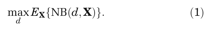
The expected value of our optimal decision, made only with current information, is
If we knew the value of the inputs of interest,
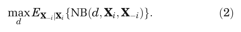
But, because
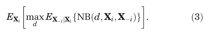
The partial EVPI for inputs
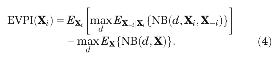
We are commonly in a situation in which we cannot evaluate any of the 3 expectations in Equation 4 analytically. Important exceptions are cases in which models are either of linear form (e.g.,
A PSA takes
The first term in Equation 4 requires more work, and unless there are analytic solutions to the expectations, the usual approach is to use a nested 2-level Monte Carlo method with
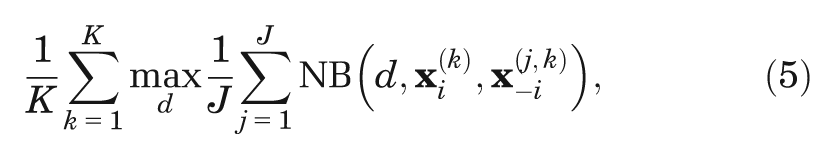
where
Sufficient numbers of runs of both the outer and inner loops are required to ensure that the partial EVPI is estimated with sufficient precision and with an acceptable level of upward bias that is induced by the maximization step. For models that are slow to run, this 2-level scheme can represent a considerable computational burden.
To address the problems of the 2-level method, we focus our attention on the estimation of the inner expectation. To avoid the need for the inner loop simulation, we reframe the estimation of this conditional expectation as a regression problem.
Principles of Estimating Partial EVPI Using Regression
Our target is to estimate the conditional expectation
First, we recognize that we can express the model output for model run
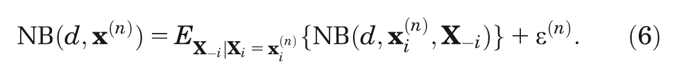
To see why the error term must have zero mean, we rearrange and take expectations,
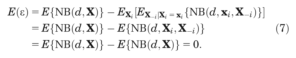
The second move is to realize that the expectation
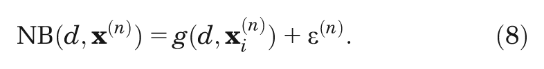
The third key idea is that we can treat the
As an illustration, Figure 1 shows the results from a hypothetical PSA in which we plot the net benefit function,
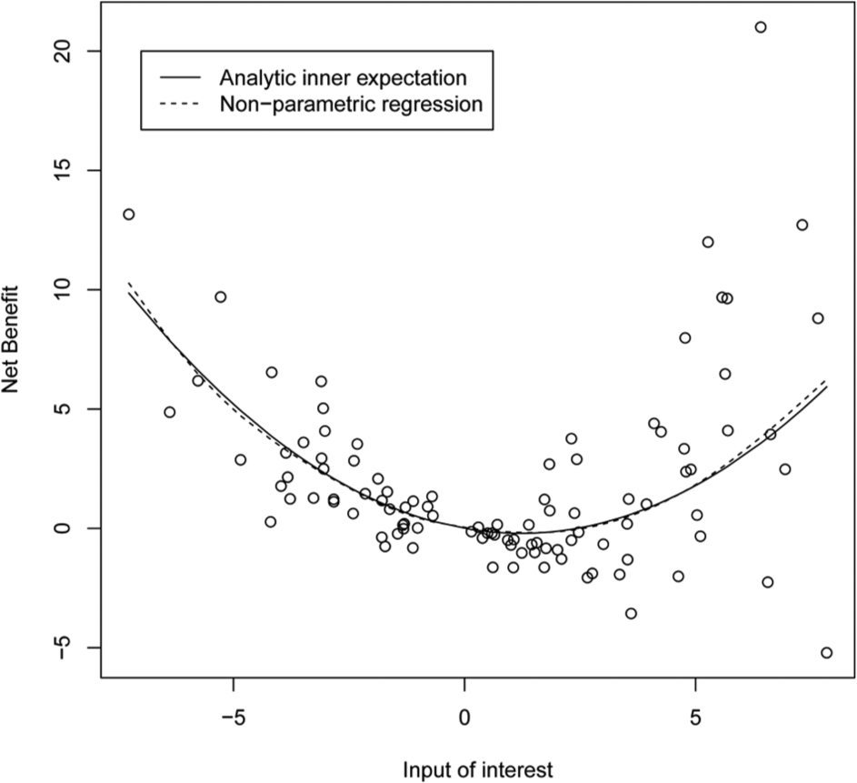
Net benefit against single input parameter of interest for hypothetical model with 3 parameters.
Once we have obtained the regression function estimate,
Note that we use
We also note at this point that EVPI (calculated by any method) is invariant to the reexpression of net benefits as incremental net benefits, relative to some chosen baseline option (which is therefore defined as having an absolute net benefit of zero). This reduces the number of regression problems from
In the next sections, we give an overview of 2 particular nonparametric regression methods that are suitable in this context, Gaussian process regression and regression based on a Generalized Additive Model (GAM).
GAM Regression
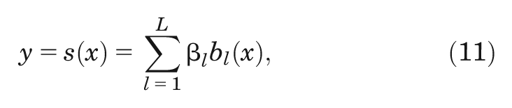
When we adopt a GAM, we represent the unknown function
where each smoothing function
The usual choice for the smoothing functions is some form of spline, a common choice being the cubic spline. A cubic spline represents an arbitrary smooth function as a series of short cubic polynomials joined piecewise, as shown in Figure 2.
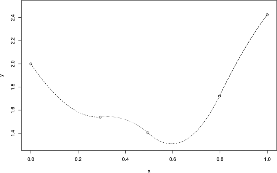
A cubic spline, showing the piecewise construction from 4 sections of cubic polynomial, each with different coefficients.
The cubic spline shown in Figure 2 can also be expressed as the weighted sum of a series of polynomial basis functions,
for some basis dimension
By expressing our unknown function (Equation 10) in the same way, we get
Estimation of the model coefficients is typically via penalized maximum likelihood, in which the penalties are designed to suppress overly wiggly estimates that would result in overfitting. The choice of basis dimension for each spline is usually not important as long as it is sufficiently large to avoid constraining the spline to be overly inflexible (we found any any dimension greater than 3 to be sufficient). In practice, the software in which GAM is implemented makes the choice of basis dimension for each spline automatically.
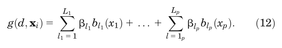
Although the simple additive model in Equation 10 performs well in many situations, it will not adequately capture interactions between the input parameters of interest that may be a feature of the health economic model. To model interactions, we must include multivariate smoothing functions in our GAM model specification. So, for example, if we expect there to be interactions between inputs
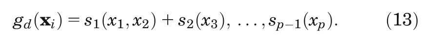
The multivariate smoothing function
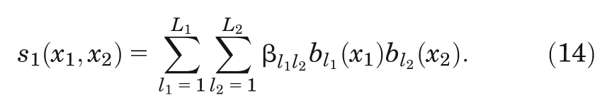
Modeling a large number of potential interactions does therefore have a cost. Given
After estimating the GAM model parameters and hence obtaining
Box 1 Example R Code for Estimating Partial Expected Value of Perfect Information via Generalized Additive Model Regression
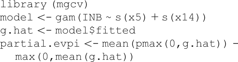
A method for estimating the standard error of the GAM-based approximation of the partial EVPI is given in Appendix A. R functions for computing the partial EVPI via GAM and its standard error are available at http://www.shef.ac.uk/scharr/sections/ph/staff/profiles/mark.
Gaussian Process Regression
The Gaussian process is a highly flexible representation of an unknown function, in our case
It is very important to note that by representing the unknown function
Until now, the use of the Gaussian process in health economics has been rare and restricted to the modeling of the net benefit function in the context of a computationally expensive model.16–18 For a practical introduction to building Gaussian process models, see the Managing Uncertainty in Complex Models toolkit at mucm.aston.ac.uk/MUCM/MUCMToolkit/.
Gaussian Process Regression Model Specification
Recall that our PSA sample consists of
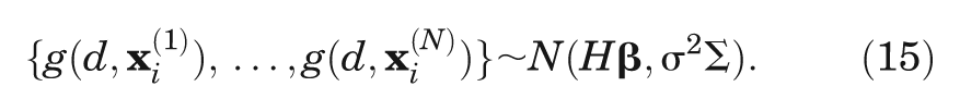
The mean of the distribution Hβ is a vector of length
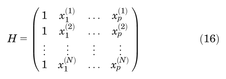
of size
We require that the correlation matrix
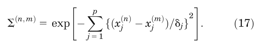
The superscripts
Note that the form of the correlation function ensures that diagonal entries in the matrix
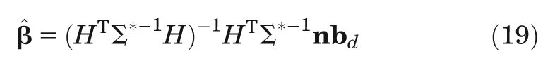
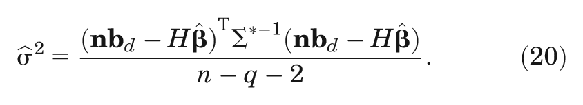
Finally, we require a method for learning about

where
Estimation of Hyperparameters
,
,
, and
The first step is to estimate the correlation lengths
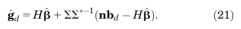
and the posterior mean of
Estimation of
Once we have determined
The components of
Implementation Issues and Regression Diagnostics
We recommended above that net benefits are expressed as incremental net benefits, relative to a chosen baseline option. This not only reduces the number of regression problems from
For both Gaussian process and GAM models, examination of the residuals is useful for assessing the robustness of assumptions. A plot of residuals (i.e.,
Case Studies
Case Study 1: A Simple Decision Tree Model with Correlated Inputs
Case study 1 is based on a hypothetical decision tree model previously used for illustrative purposes.5,7,9,10 The model predicts net benefit,

where
Summary of Means and Standard Deviations for Case Study Model Parameters
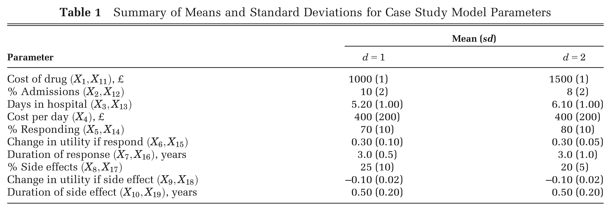
We assume that our uncertainty about the inputs can be represented by a multivariate Normal distribution, with
We define 3 parameter sets of interest: set 1 comprising effectiveness parameters
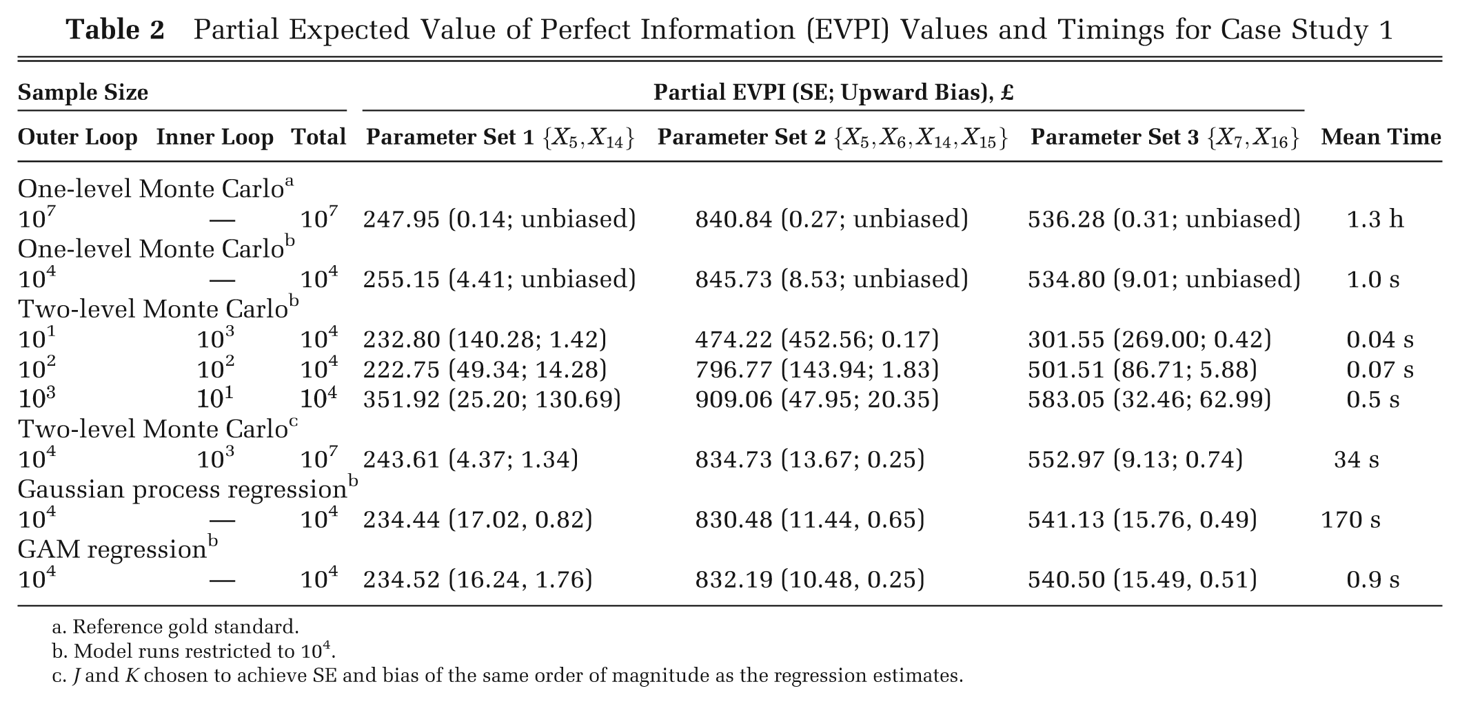
Although the case study model is computationally cheap to evaluate, we assume that we are in a position of being able to evaluate the model only 10 000 times. Given this limitation, we calculated partial EVPI using 3 methods. First, we calculated the partial EVPI for each parameter set using a single-loop Monte Carlo approximation for the outer expectation in the first term of the right-hand side of Equation 4 with 10 000 samples from the distribution of the parameters of interest, an analytic solution to the inner conditional expectation, and hence 10 000 model runs. Next, we calculated the partial EVPI values using the standard 2-level Monte Carlo approach with 3 different sets of
Partial Expected Value of Perfect Information (EVPI) Values and Timings for Case Study 1
Reference gold standard.
Model runs restricted to 104.
J and K chosen to achieve SE and bias of the same order of magnitude as the regression estimates.
We compared values with a gold standard measure of partial EVPI calculated using the analytic solution to the inner conditional expectation, and 107 outer loop samples. Standard errors for the 2-level Monte Carlo partial EVPI estimates were obtained using the method given in Appendix A. Estimates of partial EVPI using the 2-level Monte Carlo method are upwardly biased for small values of
For each method, we report the mean time taken to compute the partial EVPI for the 3 parameter sets of interest.
Results for Case Study 1
Regression diagnostic plots for the Gaussian process and GAM models are shown in Figure 3. A random subset of 500 points is shown on each plot. First of note is, for each parameter set, the similarity in the pattern of residuals between the Gaussian process model and the GAM model (reflecting the similarity in estimates of
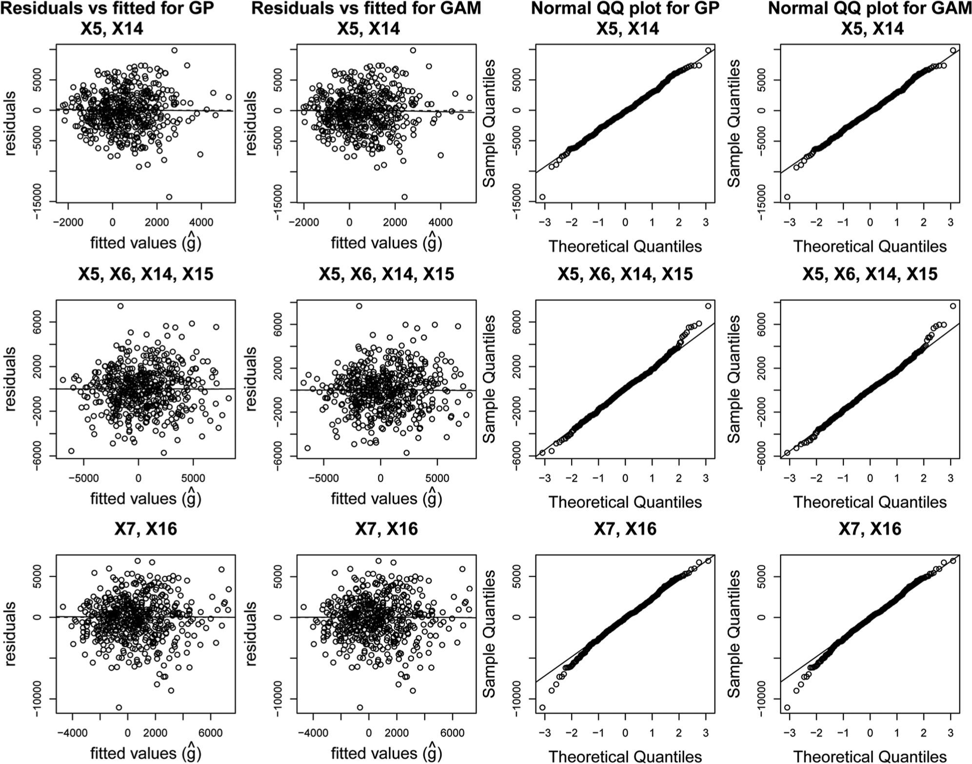
Regression diagnostic plots for case study 1.
Figure 4 shows the values of
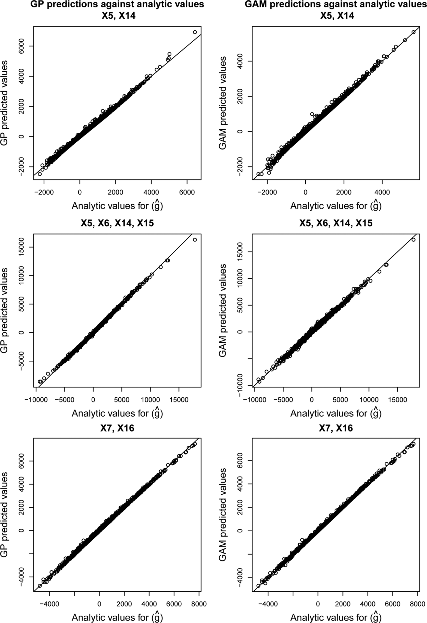
Gaussian process and Generalized Additive Model regression predictions versus analytic values for case study 1.
Table 2 shows the estimated partial EVPI values for the 3 sets of parameters of interest. The overall EVPI for all 19 parameters is £1047. The top line shows the gold standard estimates, obtained by generating 107 samples from the joint distribution of the inputs of interest and then analytically calculating the expected net benefits for each decision option, conditional on these sampled values. The standard errors of the gold standard estimates are small. When we restrict ourselves to only 10 000 model evaluations, but again use the analytic solution to the conditional expectation, the standard errors are unsurprisingly larger. The estimates are still unbiased. In contrast, estimates obtained via the 2-level Monte Carlo approach are biased due to the maximization over quantities that are subject to sampling variability. 9 When restricted to 10 000 model evaluations, there is a clear tradeoff between bias and variance when using the 2-level method, with small values of the inner loop resulting in considerable upward bias.
In comparison, the regression-based estimates all have lower variance than any of the 2-level Monte Carlo estimates when model runs are restricted to 10 000. The upward bias due to the maximization in the first term of Equation 9 is small in each case and comparable with that obtained by the 2-level Monte Carlo method with 1000 inner loop samples. To achieve a similar level of bias and variance to that obtained using the regression method with 104 PSA samples, the 2-level Monte Carlo would require approximately 107 model runs.
The computational cost of obtaining the gold standard estimate is greatest, because of the large sample size. The 2-level Monte Carlo method is fast in this example because of the simplicity of the model but will typically be slower and will increase as the computational complexity of the model increases. In contrast, the speeds of the Gaussian process and GAM methods are independent of the computational complexity of the model because the model itself is not evaluated during the regression fitting process. The GAM method takes less than 1 s with a PSA sample size of 104, whereas the Gaussian process method takes approximately 3 min.
Case Study 2: Three State Markov Model
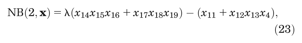
Case study 2 is an extension of the case study 1 model that incorporates a 20-time cycle Markov model for the response to each intervention. The parameters for mean duration of response (
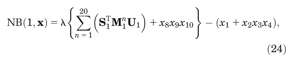
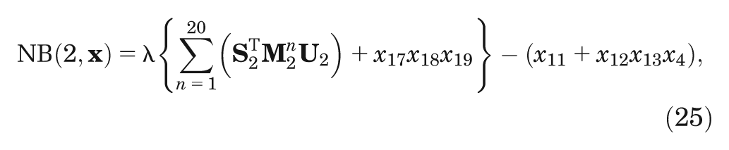
where the vectors
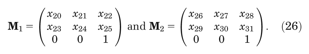
Uncertainty regarding the transition matrix parameters (
We again defined 3 parameter sets of interest: set 1 comprising effectiveness parameters
Results for Case Study 2
A similar pattern of results is seen for case study 2 as for case study 1. Regression diagnostic plots shown in Figure 5 are similar in character to the those obtained in the first case study, and again, no worrying departures from the model assumptions are indicated.
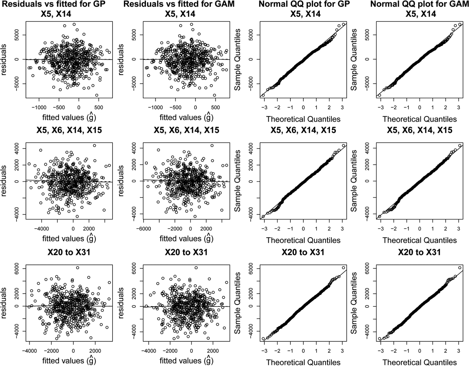
Regression diagnostic plots for case study 2.
Figure 6 shows the values of
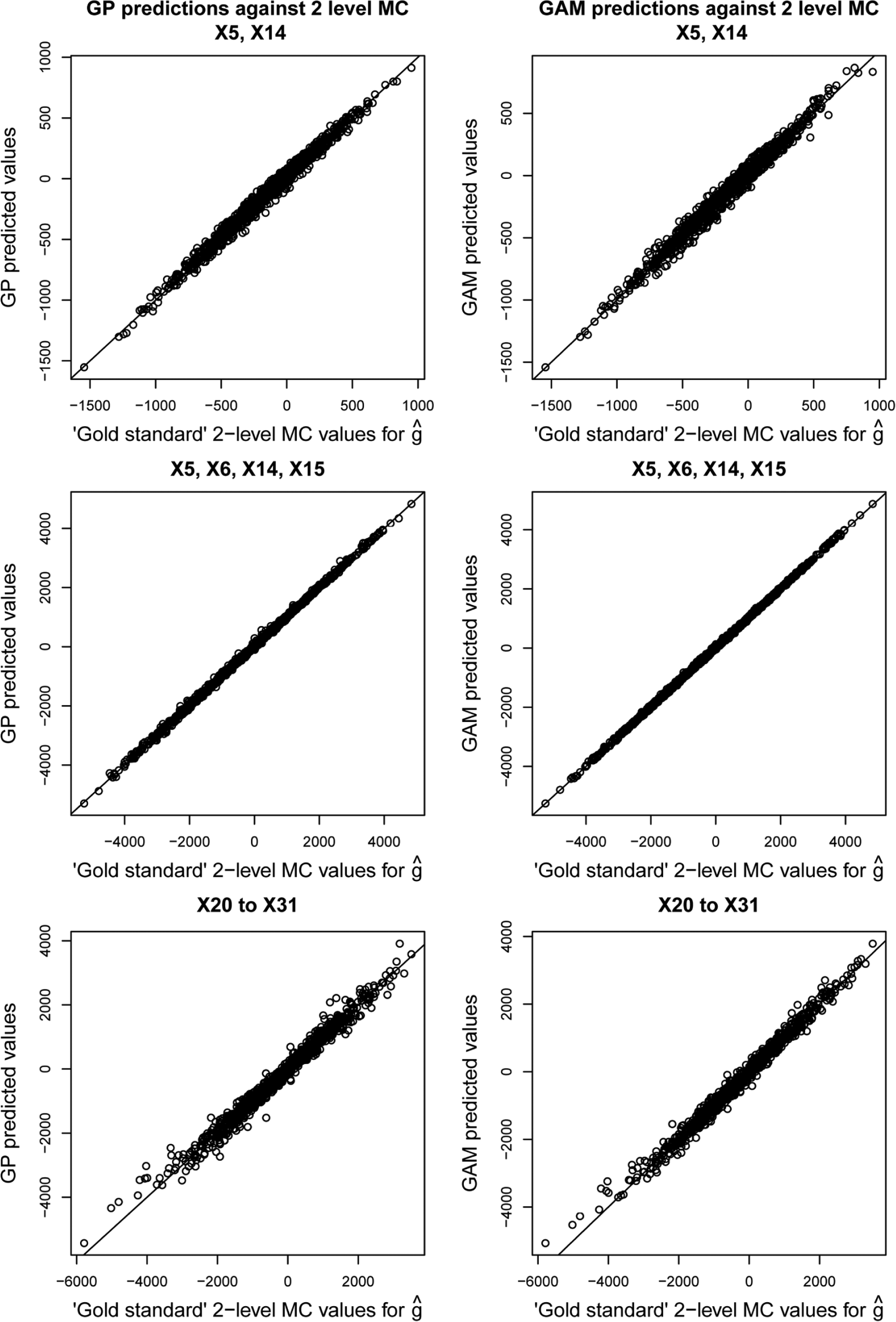
Gaussian process and Generalized Additive Model regression predictions versus those obtained via the gold standard 2-level Monte Carlo method for case study 2.
Table 3 shows the estimated partial EVPI values. The overall EVPI is £775. Standard errors for the gold standard 2-level Monte Carlo estimates with 108 model runs are small, as are the values of the upward bias. When the number of model evaluations is restricted to 104, the regression methods perform considerably better than the 2-level Monte Carlo method, resulting in estimates that have both minimal upward bias and substantially greater precision. To achieve a similar level of bias and variance to that obtained using the regression method with 104 PSA samples, the 2-level Monte Carlo would require approximately 107 model runs.
Partial Expected Value of Perfect Information (EVPI) Values and Timings for Case Study 2
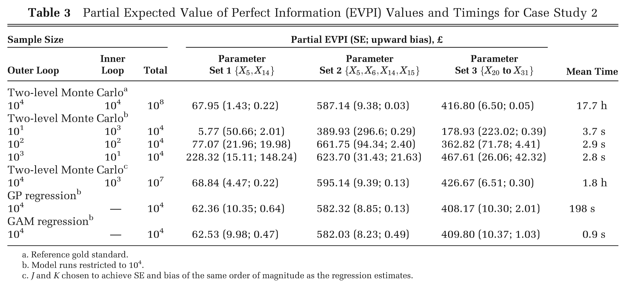
Reference gold standard.
Model runs restricted to 104.
J and K chosen to achieve SE and bias of the same order of magnitude as the regression estimates.
With a PSA sample size of 104, the GAM takes approximately 1 s and the Gaussian process takes approximately 3 min. In contrast, the 2-level Monte Carlo method with 107 model runs takes 1.8 h.
Discussion
Main Result and Implications
The regression-based approach we propose requires only the single set of model evaluations that is generated in a standard probabilistic sensitivity analysis to calculate partial EVPI for any set of inputs. It leads to a considerable gain in precision over the 2-level Monte Carlo method with the same number of model runs while retaining an acceptably small upward bias. The GAM method in particular is straightforward to implement in the freely available software R, thus allowing an analyst to compute partial EVPI for any subset of input parameters quickly and with relative ease.
The regression method allows the complete separation of the EVPI calculation step from the model evaluation step, which may be particularly useful when the model has been built using specialist software (e.g., for discrete event simulation) that does not allow easy implementation of the EVPI step or where those who wish to compute the EVPI do not own (and therefore cannot directly evaluate) the model. The method has the particular advantage that, even in the case of correlated inputs, only the joint distribution of inputs is required. This is in contrast to the 2-level Monte Carlo approach in which we are required to sample values from
In terms of computational speed, the regression methods are fast. We see 2 particular scenarios in which this will be useful: when the analyst is faced with a slow patient-level simulation model and in the case in which the partial EVPI calculation would require computationally demanding MCMC sampling under the 2-level scheme.
For health economic decision analysts, the key implication of the nonparametric regression approach is that the computation of partial EVPI has become tractable for any decision problem. We hope that the computation of partial EVPI values now becomes standard practice, and we urge those who write guidance on good modeling practice to promote the routine reporting of EVPI values.
Limitations
There are some limitations of the regression approaches. In general, the GAM method will be more straightforward to implement because of the easy availability of software (e.g., the mgcv package in R). However, if the set of input parameters for which we wish to calculate partial EVPI is moderately large (greater than 6 or so), and if it is expected that those parameters will jointly interact (nonadditively) within the economic model, then it is likely that the number of GAM model parameters that need to be estimated will exceed the number of data points, causing the method to fail. In this case, we would recommend using the Gaussian process approach.
Although the Gaussian process method is relatively easy to implement in R using the functions available at http://www.shef.ac.uk/scharr/sections/ph/staff/profiles/mark, the estimation of the hyperparameters requires numerical optimization, which will be slow if the number of parameters of interest is large. This optimization is not a black box procedure, and as with other numerical methods such as MCMC, the onus is on the user to ensure that convergence is achieved. Second, the Gaussian process method incurs the computational cost of inverting the
Using the Method in Patient-Level Models
In our introduction, we presented a typical scenario in which obtaining partial EVPI via 2-level Monte Carlo was likely to be computationally prohibitive due to the requirement to sample many thousands of patients within each evaluation of the inner loop.
Partial EVPI via the regression method is calculated for a patient-level model in the same manner as it is for a cohort model (i.e., by regressing the PSA sample net benefits on the parameters of interest). We briefly recap here the computation of a PSA for a patient-level model. This is a 2-level process whereby samples are drawn from the PSA level (i.e., population level) parameters in an outer loop, and then, conditional on these samples, individual patients are sampled in an inner loop. The purpose of sampling individual patients is to average over heterogeneity (and/or uncertainty) at the patient level for each sample of population-level input parameters. Convergence is achieved when the patient-level sample size is large enough that, given some arbitrary sample from the PSA (population)–level parameters, the estimated net benefit is stable. Nonconvergence will introduce additional noise in the estimation of the net benefit for each sample from the PSAlevel parameters.
Now, recall that in our approach, we treat all variability in the net benefit that is not due to the parameters of interest as noise (Equation 8). Any residual variability due to nonconvergence of the patient-level simulation will be treated as noise in the regression and averaged out. Because the regression estimation occurs before the maximization step, the residual first-order uncertainty will not cause an upward bias in the partial EVPI estimate.
Other Uses of the Gaussian Process in Health Economic Decision Modeling
In our method, we modeled the target conditional net benefit as an unknown smooth function of the parameters of interest. The observed net benefits in the PSA sample were treated as noisy data from which to learn about the unknown function. This use of a nonparametric regression method to approximate the (conditional) output of a health economic decision model is subtly different from the use of the Gaussian process in previous work by Stevenson and others, 16 Tappenden and others, 17 and Rojnik and Naversnik. 18 In these previous applications, the Gaussian process was used to model the net benefit itself as an unknown function of all the unknown input parameters, rather than to model the conditional net benefit as a function of the parameters of interest only. The primary purpose for using the Gaussian process was to construct a meta-model or emulator for the health economic decision model to allow a slow model to be replaced by a fast surrogate. Although this approach reduces computation time, the calculation of partial EVPI will typically still require a nested 2-level Monte Carlo approach. More importantly, this use of the Gaussian process does not address the problem of sampling from potentially difficult conditional distributions if input parameters are correlated.
Further Research
Although partial EVPI is useful in highlighting the sensitivity of the decision to any particular subset of input parameters, it represents only an upper bound on the expected value of undertaking research to reduce decision uncertainty. More useful is the expected value of sample information (EVSI), which represents the expected value of undertaking a particular data collection exercise. 11 We are currently working on extending the regression method described above to the computation of EVSI.
Conclusion
In conclusion, the regression-based approach to computing partial EVPI is likely to be of considerable benefit over the traditional 2-level Monte Carlo approach, except perhaps in models that are computationally very cheap to evaluate and in which there are no correlations in the inputs. With the increasing use of patient-level micro-simulation models, we envisage that obtaining partial EVPI via the traditional 2-level Monte Carlo approach will be considered just too time-consuming (in fact, experience suggests that the 2-level Monte Carlo procedure is considered too difficult for even moderately simple cohort models). In contrast, the regression methods we have presented provide a mechanism for rapidly estimating partial EVPI for any set of parameters in a model of any complexity.
Footnotes
This report is independent research supported by the National Institute for Health Research (Mark Strong, postdoctoral fellowship PDF-2012-05-258). The views expressed in this publication are those of the authors and not necessarily those of the National Health Service, the National Institute for Health Research, or the Department of Health.
References
Supplementary Material
Please find the following supplemental material available below.
For Open Access articles published under a Creative Commons License, all supplemental material carries the same license as the article it is associated with.
For non-Open Access articles published, all supplemental material carries a non-exclusive license, and permission requests for re-use of supplemental material or any part of supplemental material shall be sent directly to the copyright owner as specified in the copyright notice associated with the article.