Sage Journals: Discover world-class research

Abstract

Quantitative measurement of cerebrospinal fluid (CSF) flow and volume and longitudinal monitoring of CSF dynamics provide insights into the compensatory characteristics of post-stroke CSF. In this study, we compared the MRI pseudo-diffusion index (D*) of live and sacrificed rat brains to confirm the effect of ventricular CSF flow on diffusion signals. We observed the relationship between the CSF peak velocities and D* through Monte Carlo (MC) simulations to further understand the source of D* contrast. We also determined the dominant CSF flow using D* in three directions. Finally, we investigated the dynamic evolutions of ventricular CSF flow and volume in a stroke rat model (n = 8) from preoperative to up to 45 days after surgery and determined the correlation between ventricular CSF volume and flow. MC simulations showed a strong positive correlation between the CSF peak velocity and D* (r = 0.99). The dominant CSF flow variations in the 3D ventricle could be measured using the maximum D* map. A longitudinal positive correlation between ventricular CSF volume and D* was observed in the lateral (r = 0.74) and ventral-third (r = 0.81) ventricles, respectively. The directional D* measurements provide quantitative CSF volume and flow information, which would provide useful insights into ischemic stroke with diffusion MRI.

Keywords

Cerebrospinal fluid volume cerebrospinal fluid flow diffusion MRI subacute stage ischemic stroke

Introduction

A blockage in the brain artery can cause an ischemic stroke, leading to a cascade of responses. Reduced cerebral blood flow leads to blood-brain barrier dysfunction,¹ inflammation,² cerebral edema,^3,4 and cerebrovascular remodeling.^5,6 Recently, alterations in the cerebrospinal fluid (CSF) associated with ischemic stroke have been highlighted.^7–11 CSF surrounds and protects the brain from external shock and circulates in the ventricles, subarachnoid space, and perivascular spaces, communicating with interstitial fluid to remove metabolic waste products. Several studies have shown that changes in CSF volume and flow occur after a stroke. Acute (<24 hours) and subacute (∼5 days) changes in CSF volume^7–10 have been suggested as quantitative biomarkers of edema formation. Moreover, volumetric CSF analysis has been suggested for reliably assessing cerebral edema severity⁷ and facilitating accurate final infarct volume estimation.¹⁰ Regarding CSF flow, the reduction in glymphatic perfusions, such as para-arterial or para-venular flux, was observed in ischemic stroke mice 3 hours after surgery using magnetic resonance imaging (MRI) with a contrast agent.¹¹ Another study utilizing MRI and two-photon microscopy⁹ has proposed that rapid CSF inflow, triggered by ischemic spreading depolarization, along the perivascular space is a major cause of early edema after the obstruction of blood flow. Since the development of edema during the first week after stroke is dynamic,¹² these preceding studies mainly focused only on a short duration of less than 5 days after the stroke. However, subsequent longitudinal monitoring of CSF dynamics, such as CSF volume and flow changes, has been highlighted for exploring and understanding the compensatory mechanisms and functions of CSF after ischemic stroke as the alterations of the adjacent ventricle area known to occur in the subacute and chronic stages.¹³ On the other hand, simultaneous longitudinal monitoring of CSF volume and flow is rare, especially during the development of ischemic strokes in the subacute and chronic stages.

As a conventional way to measure CSF flow information, phase-contrast MRI (PC-MRI)^14–16 is often utilized for the characterization of CSF flow. However, flow measurement using 3D PC-MRI is time-consuming, and optimal respiration and heart triggering must be considered in obtaining the average flow velocity of an imaging voxel. It is also difficult to acquire detailed CSF flow characteristics, such as flow distribution, and the selection of slice orientation and location which should be perpendicular to the flow for PC-MRI¹⁴. All of the above factors pose significant burdens on monitoring flow information of ischemic brains in preclinical and clinical MRI.

As an alternative method to relieve the limitations of PC-MRI, diffusion MRI can be utilized to obtain CSF volume and flow information simultaneously within a reasonable scan time for strokes. The fast diffusion component, which reflects fluid flow, can be measured by acquiring low b values with a double-exponential decay fit curve.¹⁷ Several studies^18–20 have reported that diffusion measurements at low b values are sensitive to bulk flow, such as CSF. Additionally, as the diffusion gradient directions can be varied arbitrarily, the principal direction of the CSF flow can also be obtained.¹⁸ Regarding ventricular CSF volume measurement, T₂-weighted images are often used to quantify the CSF volume in the ventricle with voxel-based morphometry (VBM)^21,22 or manual volumetry.²³ However, cerebral infarction in ischemic strokes, which is hyperintense on T₂-weighted images, may easily interfere with the accurate quantification of ventricular volume.²⁴ Considering the reduction of diffusion in cerebral infarction,²⁴ the combination of an increase in the T₂ value and the reduction in the apparent diffusion coefficient (ADC) value may contribute to the disambiguation of CSF volume. Thus, diffusion MRI may provide a robust quantitative platform for longitudinally monitoring sophisticated CSF characteristics, such as the relationship between CSF volume and flow, which can help understand compensatory CSF function and pathological processes in ischemic stroke.

In this study, the effect of CSF flow on the diffusion signals of the ventricle at low b values was directly verified in live and sacrificed rat brains. Second, the change in the pseudo-diffusion constant (D*) according to the change in the CSF peak velocity was validated using a Monte Carlo (MC) simulation. Third, a principal directional D* map of the entire 3D ventricular structure was generated, and the changes in D* and ventricular CSF volume for up to 45 days after stroke onset were longitudinally investigated. Finally, the correlation between D* and CSF volume in the lateral and ventral-third ventricles was longitudinally monitored in an ischemic stroke model (n = 8) to highlight the ability to identify and measure CSF characteristics during the development of ischemic strokes.

Materials and methods

Animal preparation

Animal experiments were performed in accordance with the Animal Protection Act of Korea under the guidelines and regulations approved by the Institutional Animal Care and Use Committee of the Ulsan National Institute of Science and Technology. All experiments were reported in compliance with the ARRIVE guidelines (Animal Research: Reporting In Vivo Experiments).²⁵ The experiments were performed using male Wistar rats weighing 300–360 g at 9-11 weeks of age. Rats were initially anesthetized in an induction chamber with 3.5% isoflurane in 70% N₂O and 30% O₂ and maintained 1.5-2% isoflurane during 1 hour of transient middle cerebral artery occlusion (tMCAO) surgery and MR experiments. Respiration and heart rate were monitored during acquisition with a respiration pillow sensor (Small Animal Instruments Inc., NY, USA) and a foot sensor (MouseOx Plus, PA, USA) and maintained at 40-50 brpm and 350-390 bpm, respectively. To confirm the relationship between CSF flow and the MR diffusion signals at low b values, MR diffusion experiments were performed before and after sacrificing one rat. The longitudinal studies were performed before (0H) and after tMCAO surgery for up to 45 days (4H (hyperacute); D1, D3 (acute); D7, D16 (subacute); D25, D36, and D45 (chronic stage), n = 5), 7 days (n = 2), and 16 days (n = 1) in the rats with ischemic stroke. H and D represent the hours and days after surgery. Rats in the sham control group (for up to 16 days after surgery, n = 2) were operated with a similar method without the MCA occlusion to determine the effect of the operation, aging and repeated isoflurane anesthesia.

MRI acquisition

The MRI data were obtained using a 7 T MR scanner (Paravision 6, Bruker BioSpin, Billerica, MA, USA) with a 72-mm volume coil (transmit) and rat surface coil (receiver). The spin-echo echo-planar imaging (EPI) sequence was used to obtain the diffusion signal. The sequence parameters were as follows: repetition time (TR) = 3000 ms, echo time (TE) = 32.1 ms, field of view (FOV) = 20 × 20 mm², matrix size = 96 × 96, number of averages (NA) = 20, bandwidth (BW) = 2 × 10⁵ Hz, number of slices (NS) = 38, slice thickness (ST) = 0.5 mm, number of segments = 2, number of b values = 20 or 11 for comparing the diffusion signals of the tissue and ventricle in normal brains or obtaining the diffusion signal in longitudinal stroke brains with three orthogonal diffusion gradient directions (x, y, and z), respectively (effective b values = 5.9, 19.7, 31.2, 42.4, 53.4, 64.3, 75.1, 85.9, 96.5, 107.2, 117.8, 138.9, 160.0, 180.9, 196.6, 222.7, 326.5, 532.4, 788.4, 941.5 or 6.8, 32.3, 54.6, 76.4, 97.8, 119.1, 140.3, 161.4, 182.4, 534.4, 1045.9 s/mm²), and scan time = 66 minutes.

T₂-weighted images were acquired with rapid acquisition with relaxation enhancement (RARE)²⁶ to identify the ventricle and the infarction region in the brain tissue in detail. The sequence parameters were as follows: TR = 7000 ms, TE = 50 ms, FOV = 20 × 20 mm², matrix size = 192 × 192, NA = 2, NS = 38, ST = 0.5 mm, and RARE factor = 8.

T₂ maps were acquired, and used to obtain a more accurate ventricular region of interest (ROI) in conjunction with the ADC map using a multi-slice multi-echo (MSME) sequence, with the following parameters: TR = 7000 ms, number of TE = 20 (8–160 ms, equal interval), FOV = 20 × 20 mm², matrix size = 96 × 96, NS = 38, and ST = 0.5 mm.

Simulations

The MC simulation was performed to verify the correlation between the peak CSF velocity and D* from diffusion MRI using MATLAB R2019b (MathWorks, Natick, MA, USA). As the CSF velocity based on PC-MRI is often measured in an aqueduct in rodents where CSF flows in one direction due to the cylinder structure, the MC simulation was performed using in vivo rat experimental data from the aqueduct region. Each temporal CSF flow pattern with different peak velocities from 0.08 cm/s to 0.52 cm/s was generated based on PC-MRI of the rat aqueduct region in a previously reported study.²⁷

The simulation pipeline is shown in Supplementary Figure 1. First, a flow distribution was generated by using the flow distribution model in the aqueduct region with the assumption to be laminar.^28,29 The mean velocity of the laminar flow profile was set to be equal to the randomly sampled CSF velocity from the temporal CSF flow pattern. To approximate the in vivo experimental conditions, the CSF velocity was continuously updated with incremental time (dt) along the temporal CSF flow pattern. In the aqueduct region, the CSF dominantly flowed into the fourth ventricle along the z direction; therefore, the spins were set to flow only along the z direction in the simulation, and the CSF volume fraction was set to 100%. The ADC value (2,165 µm²/s) in the simulation was set based on the measured value in the aqueduct of a normal rat brain in an in vivo experiment. Subsequently, to calculate the phase difference between the first and last positions of the spins after the spin movement, 10⁶ spins were initially assigned to the origin (x, y, z = 0). The spin movement consists of two components: flow and diffusion. While each spin flowed at a different velocity along the laminar flow profile, it diffused randomly, following a normal distribution with a standard deviation of ${(2 \cdot ADC \cdot d t)}^{1 / 2}$ . In this simulation, $d t$ , gradient duration ( $δ$ ), and the time interval between the beginning of the two diffusion gradients ( $Δ$ ) were set to 0.1, 2, and 12 ms, respectively. The spin phases were calculated according to the RF pulses and diffusion gradients, and the average magnitude of all the spin phases was converted to signal intensity.³⁰ The diffusion signals with b values ranging from 0 to 1,148 s/mm² were obtained by calculating the average magnitude of the spin phases. As NA was 20 in the in vivo experiment, the simulation was repeated 20 times with randomized CSF velocities for each time, and the results were averaged. Single-exponential decay curve fitting was performed with the MR signal to acquire the corresponding theoretical D*. The simulations were repeated ten times by varying the CSF peak velocities, and Pearson’s correlation coefficient for the average D* and the CSF peak velocity was estimated.

Data analysis

Generation of the ventricular ROI

Before generating of the ventricular ROI, motion correction procedures for diffusion data were performed using Matlab. The details for the generation of the ventricular ROIs are described in Supplementary Figure 2. The ventricular ROI of each slice was obtained using the T₂ and ADC maps. Each ADC value along three diffusion gradient directions was obtained from a single-exponential equation ( $S_{b} = S_{0} e^{- bADC}$ ) at a given whole b value, and the average ADC value of three directions was used. First, the ventricular ROIs were obtained using a thresholded T₂ map (T₂ > 0.65 s).³¹ However, because the mask of the thresholded T₂ map contains both ventricular and edematous regions with high T₂ values, the ADC map was used to exclude the edematous regions. The high ADC mask (ADC > 0.8 × 10⁻³ mm²/s) was multiplied by the thresholded T₂ map mask to obtain the ventricular ROI. Afterward, the obtained ventricle masks were manually separated into the lateral and ventral-third ventricular ROIs. Ventricular ROIs for all rats in the tMCAO and sham group were obtained for each time point with the same procedure described above.

Generation of the maximum D* direction and maximum D* maps

The diffusion signal intensity of each ventricular ROI was fitted with a single-exponential equation ( $S_{b} = S_{0} e^{- b D^{*}}$ ) at low b values (<200 s/mm²) to obtain D* along three diffusion gradient directions. D* for each of the three diffusion gradient directions was calculated, and the direction of the main D* was determined by choosing the direction with maximum D* along three directions and labeled with the respective colors (x: red, y: blue, and z: green). The maximum D* direction map was shown in axial and sagittal views to visualize the dominant CSF flow direction in the ventricles. To generate the maximum D* map for the visualization of the extent of CSF velocities along the maximum D* direction, the corresponding D* for the selected direction was assigned for each voxel. A 3D maximum D* map was generated with a color-scaled D* along the corresponding maximum direction for each voxel. D* were normalized to an empirical value (0.004) that could provide a contrast between normal and stroke brains, and normalized D* were assigned to the RGB channels along each dominant direction for visualization. Red, green, and blue represent the x, z, and y directions, respectively.

Longitudinal follow-ups of the ventricular CSF volume and flow for the tMCAO model

The dynamic evolution of the median of D* in ventricular ROI and ventricular CSF volumes were longitudinally monitored for the lateral ventricle and ventral-third ventricle; the monitoring started before and ended 45 days after the surgery. Each ventricular CSF volume was calculated as the number of voxels in the ventricular ROI multiplied by the voxel volume 0.208 × 0.208 × 0.5 mm³. To investigate the relationship between the ventricular CSF volume and D*, Pearson’s coefficient was calculated for the correlations of the lateral ventricle and the ventral-third ventricle along the x, y, and z direction, respectively.

Results

The effect of CSF flow on diffusion signals

To investigate the effect of CSF flow on the diffusion signals, the ventral-third ventricle (red line) and the brain tissue (yellow, manually drawn) regions were drawn as shown in Figure 1(a), and the corresponding diffusion signals along the x, y, and z directions are shown in red, blue, and green colors, respectively. First, the diffusion signals fitted with the double-exponential model in the ventricular CSF (ventral-third ventricle) and tissue regions are plotted with solid and dotted lines in Figure 1(b), respectively. The diffusion signal in the ventricular CSF region decayed faster than that in the tissue region. The diffusion signal in the ventricular CSF region for each of the three directions has distinct double-exponentiality, which indicates that the diffusion signal contains flow components (D* term). The signal along the y direction decreased the most rapidly where the CSF in the ventral-third ventricle mainly flowed along the y direction. Second, the diffusion signals before and after sacrifice are plotted in the ventricular CSF region (ventral-third ventricle) with solid and dotted lines in Figure 1(c), respectively. The diffusion signal attenuation rates for the x, y, and z directions were distinguished for live animals, but they were significantly decreased and indistinguishable for the sacrificed animal, which indicates that the diffusion signal in the ventricle at low b values contains directional CSF flow information.

Figure 1.

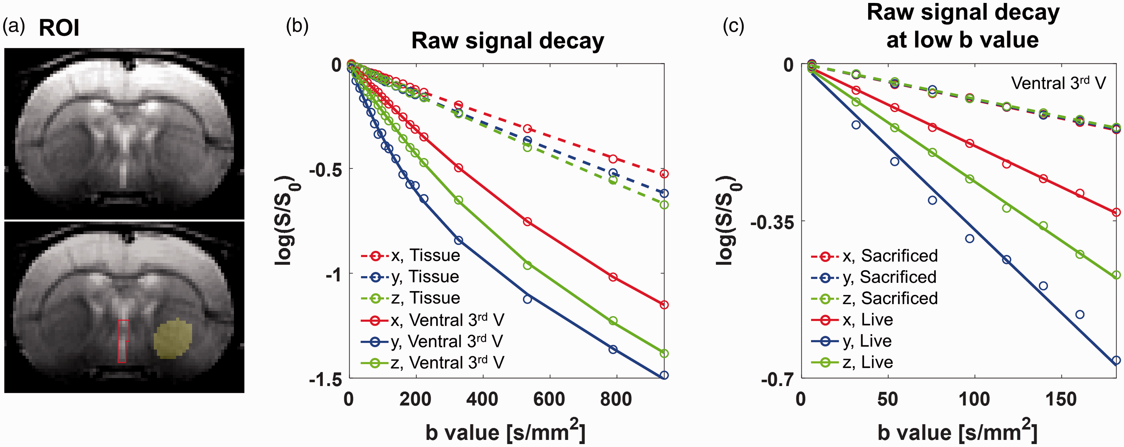
(a) ROIs with a red line and yellow-colored circle show the ventral-third ventricle and tissue regions, respectively, in a T₂-weighted image. (b) Average signal intensity (dots) and double-exponential fitted curves with respect to b values are plotted for the tissues (dotted line) and ventral-third ventricle (solid line) along different diffusion gradient directions (x: red, y: blue, and z: green). (c) Average signal intensity (dots) and single-exponential fitted curves for the ventral-third ventricle with only low b values(< 200 s/mm²) are plotted for the sacrificed (dotted line) and live (solid line) rats along three diffusion gradient directions.

Correlation between the CSF peak velocity and D* using MC simulation

To determine the correlation between the CSF velocity and D*, the CSF peak velocity was set differently from 0.08 cm/s to 0.52 cm/s by multiplying the temporal CSF flow by a constant ratio as shown in Figure 2(a). Each temporal CSF flow pattern is plotted using different colors. It is also assumed that the laminar flow was maintained. D* corresponding to each CSF peak velocity plot was obtained using MC simulations. In Figure 2(b), the averaged D* obtained over ten repetitively randomized simulations is indicated by dots of the same color corresponding to each CSF peak velocity, and the corresponding standard errors are plotted as gray error bars. A positive linear correlation was observed between the CSF peak velocity and D* (r = 0.99).

Figure 2.

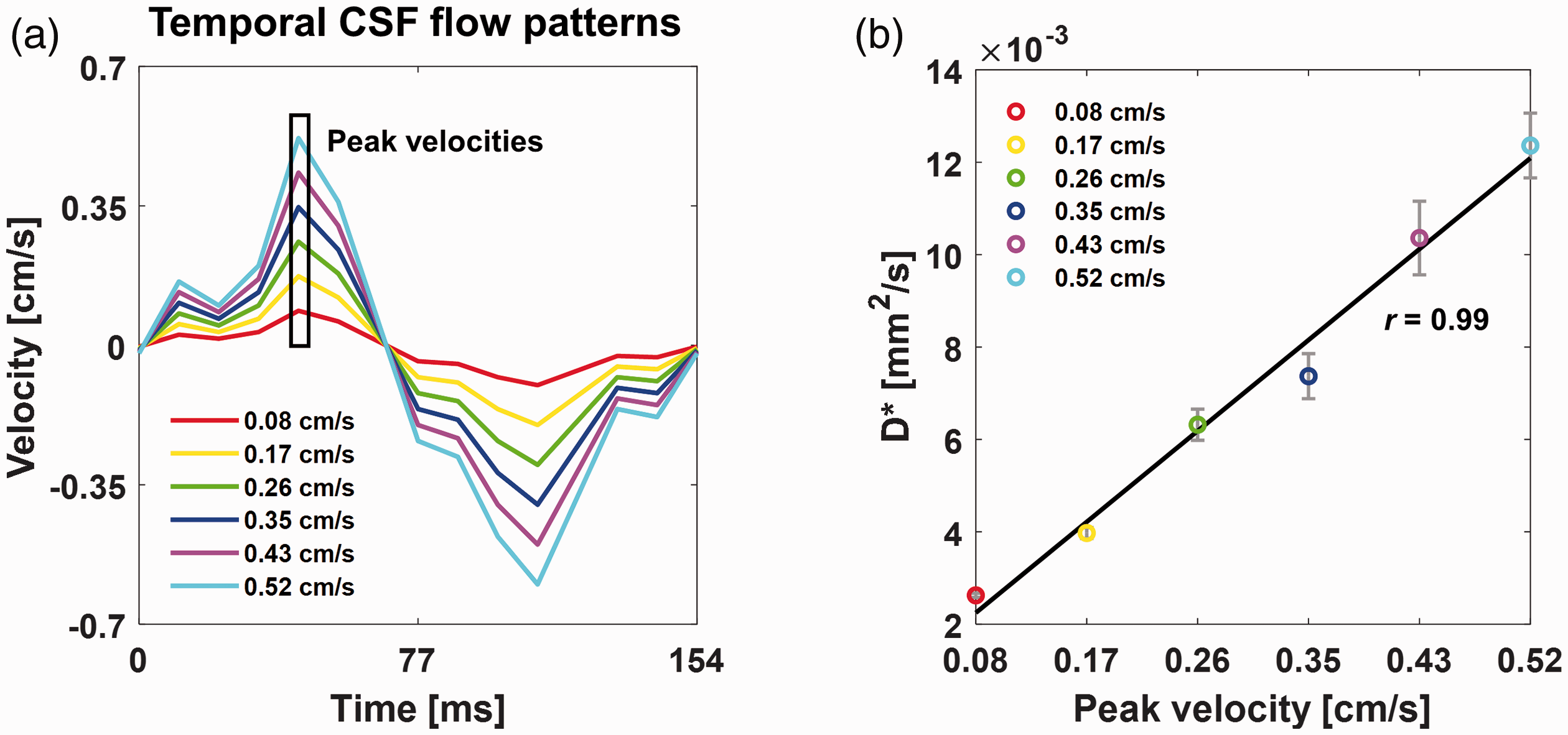
(a) The temporal CSF flow patterns were used as inputs for the corresponding Monte Carlo simulation with peak velocities ranging from 0.08 cm/s to 0.52 cm/s. (b) Plots showing the correlation between the peak velocity and averaged D* (r = 0.99) are shown. Simulations were performed 10 times with varying CSF peak velocities. The standard errors are plotted as gray error bars.

CSF flow direction detection with diffusion signal

In general, CSF has a high signal intensity in T₂-weighted images (Figure 3(a)) because its T₂ is larger compared to the tissue region, and the ventricular CSF region can be well-delineated with orange lines in a normal rat brain. In Figure 3(b), the maximum D* direction map for each voxel within the ventricular region is shown as a dot, based on the direction with the largest D*. Red, blue, and green dots represent the x (left-right), y (dorsal-ventral), and z (cranial-caudal) directions, respectively. After classifying all voxels within the entire 3D ventricular structure into three dominant flow directions, the averaged diffusion signal for each direction in the entire ventricle is plotted for the red, blue, and green dots, respectively, and they were fitted with a single-exponential decay model for low b values (Figure 3(c)). As shown in Figure 3(c), the diffusion signals along the x, y, and z directions showed the fastest decay for red, blue, green dots from the maximum D* direction map in the ventricle. These results indicate that the dominant CSF flow direction in the entire ventricle can be consistently represented with a maximum D* direction map.

Figure 3.

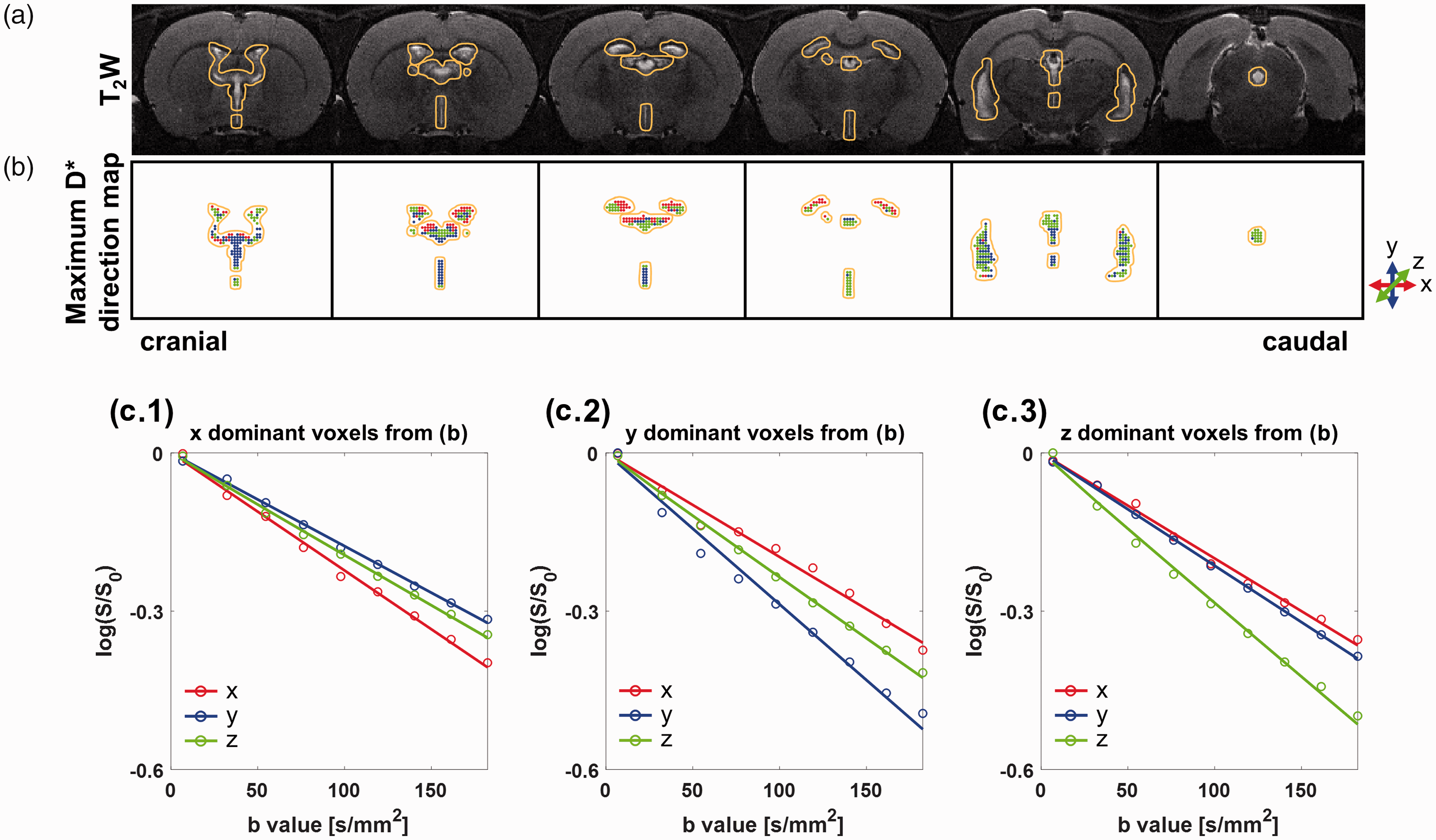
(a) Ventricle regions are indicated by orange lines on a T₂-weighted image for each slice. (b) The maximum D* direction maps with colored dots (x: red, y: blue, and z: green) indicating the direction of the largest D* for each voxel are shown. The exterior of the ventricular ROI is indicated by the identical orange outline as in (a). Average signal intensity (dots) and single-exponential fitted curves with respect to b values (< $200 s / m m^{2}$ ) are plotted for all voxels in the entire ventricle specified as dominant along each direction (x (c.1), y (c.2), and z (c.3)) in (b).

The schematic structure of the entire ventricular system of the brain is illustrated in Figure 4(a). The above and below figures represent the ventricular structures in axial and sagittal views. Black, sky-blue, yellow, and pink open boxes cover the lateral ventricle, dorsal-third ventricle, ventral-third ventricle, and aqueduct, respectively. Figure 4(b) shows the maximum D* direction maps obtained from a normal rat. The colored arrows in Figure 4(a) represent the known principal direction of the CSF flow for each ventricular region. As shown in the case of the lateral ventricle within the black open box in Figure 4(b), the group of red dots from the maximum D* direction map in the upper region corresponds well to the known principal CSF direction (red arrow) in Figure 4(a). The regions on the left side within the black open box show groups of blue and green dots, which were also well-matched with the known principal CSF directions. The principal directions for the maximum D* in the third ventricular region, which consists of two arches encircling the middle region, are y and z, which corresponded well with the known CSF flow directions. Furthermore, the main direction of the pink open box in Figure 4(b) is parallel to the narrow aqueduct structure. The principal direction from the maximum D* map is aligned with the structural shape of the ventricle. Next, a 3D maximum D* map was generated with a color-scaled D* along the corresponding maximum direction for each voxel (Figure 4(c)). As indicated by the accompanying color-scale bars, the aqueduct region with a pink open box had a brighter color than the nearby regions, which indicates that CSF flow in the pink box is faster along the z direction than in any other region.

Figure 4.

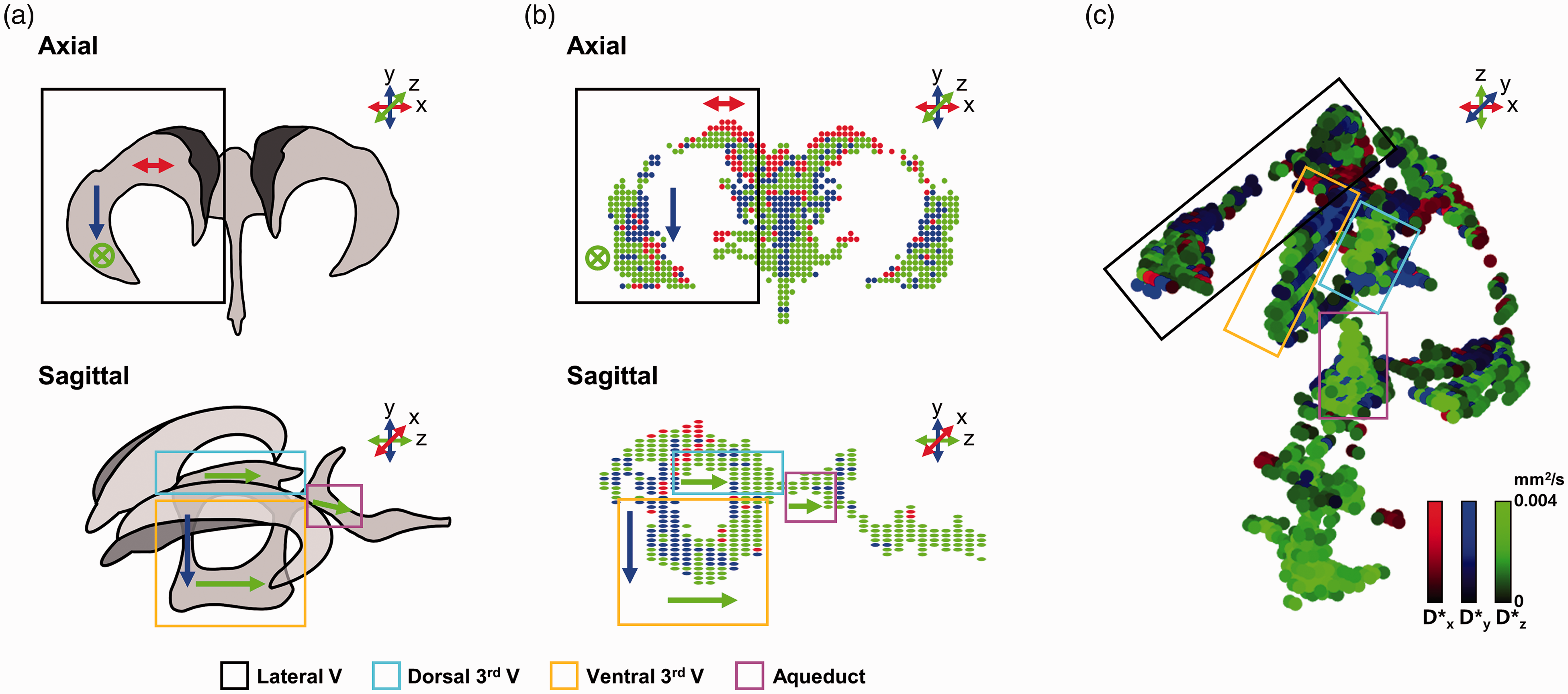
(a) Schematic of the ventricle in axial (top) and sagittal (bottom) views are illustrated. (b) The maximum D* direction map in the axial (top) and sagittal (bottom) views were generated. The arrows in the ventricle in (a) and (b) represent the known and expected dominant CSF flow directions, respectively. (c) A 3D maximum D* map represents both the direction of the largest D* by color and D* (0 to 0.004 mm²/s) by brightness within each voxel. Each ventricular region is covered with a colored box (black: lateral ventricle, sky-blue: dorsal-third ventricle, yellow: ventral-third ventricle, and pink: aqueduct).

Longitudinal study of an ischemic stroke model; changes in ventricular CSF volume and D*

Figure 5 shows the dynamic evolution of ventricles from before surgery to 45 days after surgery in a representative ischemic stroke model. And individual changes in ventricular CSF volume and D* were presented for a total of 5 rats for up to 45 days before and after tMCAO surgery in the Supplementary Figure 3. T₂-weighted images and corresponding ADC maps after surgery are shown in Figure 5(a) and (b), respectively. The edema region was observed using ADC maps, and ventricular CSF was observed using the T₂-weighted images. In this representative model, the ADC values in the ipsilateral region were significantly lower than those in the contralateral region 4 hours after surgery, and they recovered slightly on day 1 after surgery, but the damaged region was spread to a wider area on day 1. The ADC values in the ipsilateral region seemed to be pseudo-normalized 3 days after surgery. Nonetheless, the ADC values in part of the ipsilateral region were even higher than those in the contralateral region, presumably due to the progress of vasogenic edema after 7 days of surgery.³² These ADC and edema volume variations are well represented in all five subjects of the tMCAO model, as shown in Supplementary Figure 5. Accordingly, the ventricular CSF volumes containing the lateral ventricle and ventral-third ventricle in this slice have considerably changed. The maximum D* direction maps for the selected ventricular ROI with the black square are shown in Figure 5(c). The reduced CSF volume in the ventral-third ventricle on day 1 and the swollen CSF volumes in the lateral and ventral-third ventricles on day 16 were observed. Figure 5(d) shows the magnified maximum D* maps of the central ventricular region, including the ventral-third ventricle, dorsal-third ventricle, and aqueduct. The sky-blue, yellow, and pink open circles indicate the dorsal-third ventricle, the front part of the ventral-third ventricle, and the front part of the aqueduct, respectively. D* of the three ventricular areas gradually decreased and increased again from day 7.

Figure 5.

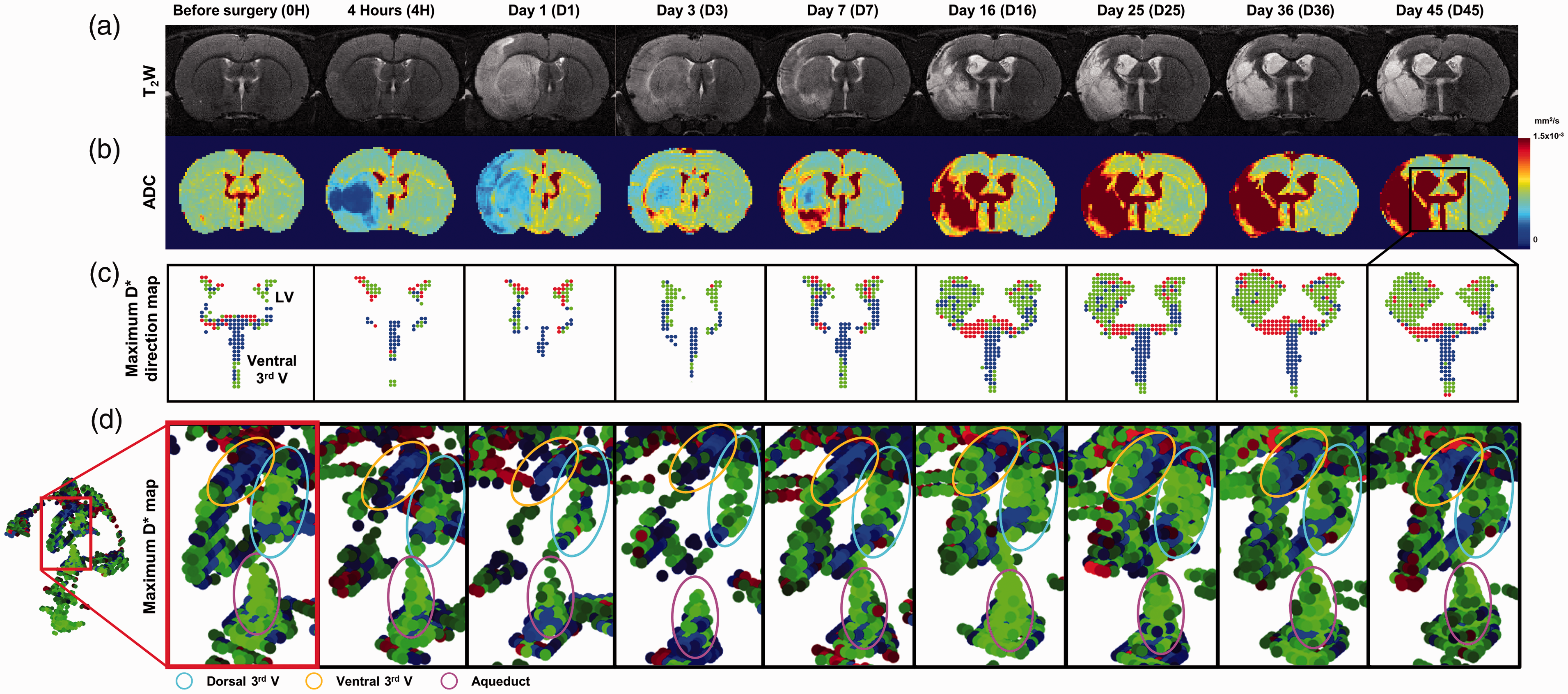
T₂-weighted images (a) and ADC maps (b) before and after surgery (up to day 45) are shown. (c) The maximum D* direction maps for each time point within the ventricle ROI were generated. (d) Magnified maximum D* direction map containing the dorsal-third ventricle (sky-blue circle), ventral-third ventricle (yellow circle), and the aqueduct (pink circle) of the 3D ventricular structure shows the main CSF flow direction and D* variations.

Correlation between ventricular CSF volume and D*

To investigate the correlation between ventricular CSF volume and D*, the lateral and ventral-third ventricular regions were selected as shown in Figure 6(a). The ventricular CSF volume and D* were longitudinally monitored in the tMCAO model (before and after surgery up to 45 days) and in the sham control group (before and after surgery up to 16 days, n = 2) as shown in the Figure 6(b) and Supplementary Figure 4(a) and (b), respectively. The longitudinal changes in ventricular CSF volume and D* in each direction of the representative model shown in Figure 5 are shown in Figure 6(b). The ventricular CSF volumes are plotted with a black line and open circles. D* values in the x, y, and z directions are plotted with red, blue, and green colored lines and open circles, respectively. For the lateral ventricle shown in Figure 6(b.1), the ventricular CSF volume and D* significantly increased from the seventh day after surgery. However, for the ventral-third ventricle shown in Figure 6(b.2), the ventricular CSF volume and D* decreased until day 1 and bounced back after day 1. The correlations between the ventricular CSF volume and D* of the lateral and ventral-third ventricles for 8 rats along the x, y, and z direction are plotted in Figure 6(c.1) and (c.2), respectively. For both the lateral and ventral-third ventricles, strong positive correlations between the ventricular CSF volume and D* were observed for all directions (r = 0.72 (x), 0.72 (y), 0.74 (z) and 0.81 (x), 0.80 (y), 0.81 (z), respectively).

Figure 6.

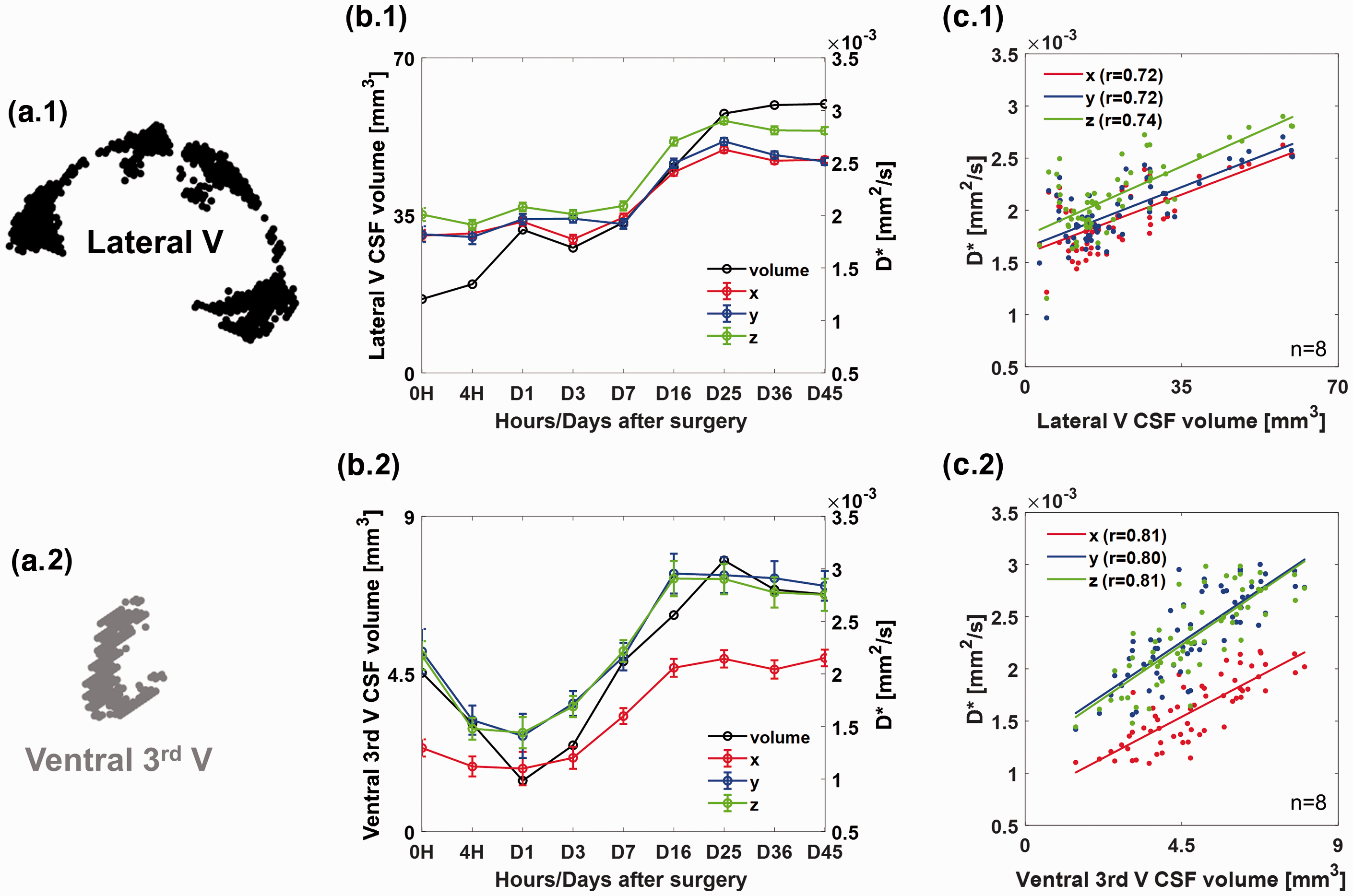
The lateral (black) (a.1) and ventral-third (gray) (a.2) ventricles were manually segmented. The changes in ventricular CSF volume, median D* and standard errors according to the diffusion gradient directions for the lateral (b.1) and ventral-third (b.2) ventricles from before surgery and up to day 45 after surgery are shown. Correlation plots for ventricular CSF volume and D* along the x (red), y (blue), and z (green) direction for the lateral and ventral-third ventricles are shown in (c.1) and (c.2), respectively. Pearson’s correlation coefficients (r) are 0.72 (x), 0.72 (y) and 0.74 (z) for lateral ventricle and 0.81 (x), 0.80 (y), and 0.81 (z) for ventral-third ventricle.

Discussion

The CSF diffusion signal showed a clear double-exponentiality attributed to the rapid reduction in the signal at low b values. As in the previous flow phantom study,³³ which confirmed the effect of the phase mismatch derived from the flow distribution on the amplitude reduction of the diffusion weight sequence, the effect of CSF flow on the signals low b values can be observed by comparing the CSF signals of the brains of live and sacrificed rats. Since the sacrificed brain had no flow of intravital fluids, including CSF, the signals of the ventricle of the sacrificed brain decayed more slowly than those of the live brain, and there was no signal difference according to the diffusion gradient direction. On the other hand, the difference in the signal decay rate at low b values along the direction of the diffusion gradient was distinct in the live brain. These results showed the directional dependence of fluid movement on D* within the ventricle, which is consistent with the report of a previous validation study.¹⁸ When the diffusion gradient direction, which is consistent with the anatomical ventricular orientation, was applied, D* was significantly higher than for other directions. The direction with the highest D* within the voxel was designated as the main CSF flow direction, and the main CSF flow direction in the segmented ventricle corresponded well with the conventional CSF flow direction detected in the cilia-based^34,35 and gadolinium-based invasive studies.³⁶

Additionally, the MC simulation results provided better insights into the cause of D* contrast at low b values. As previously reported^17,37 that D* is dependent on capillary blood flow, the simulation results showed that D* obtained from single-exponential decay fitting at low b values was directly related to the CSF flow velocity in the ventricles. According to these results, several ventricular regions of the ischemic stroke model (Figure 5(d)) showed changes in D* in the same region over time, which can be related to the changes in CSF velocity. Similar to our experimental observations, the studies^9,11 showed changes in the CSF tracer influx in the ipsilateral hemisphere after ischemic stroke, but the results were limited to the perivascular space only for a short period. Although there are still few observations of the 3D CSF flow changes in the entire ventricle after ischemic stroke, D* obtained using diffusion MRI is an important quantitative biomarker; it robustly provides CSF flow information with a few additions of low b values for diffusion MRI acquisition and post-processing.

To the best of our knowledge, the longitudinal evolutions of both CSF volume and flow (via D*) in each ventricle from the acute to chronic stage in ischemic stroke brains have been rarely reported. Distinct changes in ventricular CSF volume and flow were observed continuously during subacute (1 week to 3 weeks) and chronic (more than 3 weeks) stages. The longitudinal monitoring of both ventricular CSF volume and flow would be crucial for understanding and elucidating the compensatory CSF mechanisms for circulation dysfunction due to vascular occlusion.

It is particularly important to note that D* and the CSF volume for lateral and ventral-third ventricles have positive and linear correlations in ischemic stroke models. Previous studies^38–40 on other diseases, such as hydrocephalus and mucopolysaccharidoses, also reported that CSF flow was associated with and affected ventricular size. For ischemic stroke, the blockage of the MCA may cause a change in CSF flow,^9,11 resulting in a change in intraventricular pressure. These changes in pressure may cause compensatory changes in the ventricular volume.⁴¹ Alternatively, tissue integrity from edema can change the pressure balance between the brain tissue and ventricle within the skull, which may induce the dilation and contraction of the ventricle. The brain edema is classified into cytotoxic and vasogenic edema. In a stage of cytotoxic edema, the extracellular ion balance is disrupted, causing the cells to swell, which lowers the ADC in that region.^42–44 These changes caused by cytotoxic edema eventually affect the pressure balance between the tissue and ventricle. The swollen cells can compress the ventricle by elevating intracranial pressure,^45,46 which may reduce the ventricular volume, such as the contraction of ventral-third ventricle between 4 hours and 3 days after surgery in this study. For the vasogenic edema, the extracellular space is swollen due to the breakdown of the blood-brain barrier (BBB).^44,46 At this stage, the ventricles may dilate due to disruption of the CSF circulation caused by a damaged nerve system.⁴⁷ Alternatively, the CSF pressure in the ventricular structures may decrease to increase the clearance of edema, resulting in ventricle enlargement.⁴⁸ As in previous studies, our further study confirmed the effect of edema on ventricular volume through changes in ADC and edema volume (Supplementary Figure 5). Cytotoxic and vasogenic edema ROIs were obtained using the combination of thresholded T₂ and ADC maps. The ventral-third ventricle volume was shrunk the most when the cytotoxic edema volume was largest, and the ventral-third ventricle volume increased as the vasogenic edema volume increased. Thus, we observed that the ventral-third ventricle can be significantly affected by the type and volume of edema. However, it is difficult to completely isolate the volume change due to the effects of stroke because the enlargement of the lateral ventricle may be affected by aging, as shown in the Supplementary Figure 4. Such changes in ventricular volume may also invoke associated CSF flow changes. In addition, the response of the choroid plexus (CP) that produces and secretes CSF after ischemic stroke may be attributed to changes in ventricular CSF volume and flow. Several studies^49–52 have reported that if CP is not directly affected, it can detect and respond to brain injury, probably due to the reduction of blood flow in CP or changes in CSF composition. There are few studies on possible CSF production changes after stroke, and the protective or compensatory mechanisms associated with CP are still unclear. However, it has been speculated that changes in the CSF production rate along with changes such as growth factor production⁵⁰ and cell proliferation rate⁵² may cause changes in overall CSF characteristics, which may affect ventricular CSF volume and flow. Alternatively, CP in the lateral and third ventricles can be directly damaged by stroke, and malfunction or morphological changes in CP can influence changes in the CSF dynamics. However, since various causes may influence the characteristics of CSF or changes in ventricular volume, further studies are needed to determine the relationships between various factors such as CSF flow, intraventricular or intracranial pressure, and ventricular CSF volume in each ventricle in ischemic stroke brains.

This study has several limitations. First, the number of diffusion gradient directions was limited to three to reduce the MR scan time. However, three orthogonal diffusion gradient directions were observed to be sufficient to estimate the projection of the principal CSF flow direction, and increasing the number of diffusion gradient directions can provide more sophisticated flow information for ventricular structures as well as the circle of Willis, perivascular space and cistern regions which CSF flows. Second, the effective number and distribution of low b values were not optimized. The optimization of the number and distribution of the b values for observing the CSF characteristics should be investigated to shorten the scan time and immediate translation to the clinic. Third, there was no direct comparison of independent CSF velocity and D* in the in vivo experiment. A comparative study of CSF velocity (possibly from 3D PC-MRI) and D* may further characterize CSF flow, such as distributions. Fourth, the separated CSF volume, especially the narrow third ventricle can be slightly over/under-estimated due to the partial volume effect. Accurate ventricular volume acquisition requires partial volume correction or VBM using images of varying contrast and higher spatial resolution.

In summary, our study demonstrated that directional CSF flow has a distinct effect on diffusion signals, and the voxel-wise maximum D* map within the entire 3D ventricle can be successfully visualized to simultaneously investigate changes in ventricular CSF volume and flow in normal and tMCAO rat models from the acute to chronic stages. The simulation results showed a strong relationship between the CSF peak velocity and D* obtained from the diffusion signals, indicating that D* can serve as a quantitative indicator of the flow and the pathological state of the brain. Finally, D* and CSF volume changes were linearly correlated in the ischemic stroke model, which may provide insights into the compensatory CSF behaviors during the pathologic process of ischemic stroke.

Supplemental Material

sj-pdf-1-jcb-10.1177_0271678X211060741 - Supplemental material for D* from diffusion MRI reveals a correspondence between ventricular cerebrospinal fluid volume and flow in the ischemic rodent model

Supplemental material, sj-pdf-1-jcb-10.1177_0271678X211060741 for D* from diffusion MRI reveals a correspondence between ventricular cerebrospinal fluid volume and flow in the ischemic rodent model by MinJung Jang, SoHyun Han and HyungJoon Cho in Journal of Cerebral Blood Flow & Metabolism

Footnotes

Funding

The author(s) disclosed receipt of the following financial support for the research, authorship, and/or publication of this article: This work was partially supported by the National Research Foundation of Korea grants from the Korean government (Nos: 2018R1A6A1A03025810 and 2018M3C7A1056887). This study was partially supported by a grant of the Korea Healthcare Technology R&D Project through the Korea Health Industry Development Institute (KHIDI), funded by the Ministry of Health & Welfare, Republic of Korea (grant No: HI14C1135). This research was also partially supported by the ‘2021 Joint Research Project of Institutes of Science and Technology’.

Declaration of conflicting interests

The author(s) declared no potential conflicts of interest with respect to the research, authorship, and/or publication of this article.

Authors’ contributions

MJJ, SHH, and HJC designed the experiments. MJJ and SHH collected and analyzed the data. MJJ, SHH, and HJC wrote the paper together.

Supplemental material

Supplemental material for this article is available online.

References

Jiang

Andjelkovic

Zhu

, et al. Blood-brain barrier dysfunction and recovery after ischemic stroke. Prog Neurobiol 2018; 163–164: 144–171.

Campbell

De Silva

Macleod

, et al. Ischaemic stroke. Nat Rev Dis Primers 2019; 5: 1–22.

Dostovic

Smajlovic

, et al. Brain edema after ischaemic stroke. Med Arch 2016; 70: 339–341.

Thorén

Azevedo

Dawson

, et al. Predictors for cerebral edema in acute ischemic stroke treated with intravenous thrombolysis. Stroke 2017; 48: 2464–2471.

Liu

Wang

Akamatsu

, et al. Vascular remodeling after ischemic stroke: mechanisms and therapeutic potentials. Prog Neurobiol 2014; 115: 138–156.

Kang

Jin

Lee

, et al. MRI visualization of whole brain macro-and microvascular remodeling in a rat model of ischemic stroke: a pilot study. Sci Rep 2020; 10: 1–12.

Dhar

Yuan

Kulik

, et al. CSF volumetric analysis for quantification of cerebral edema after hemispheric infarction. Neurocrit Care 2016; 24: 420–427.

Dhar

Chen

Hamzehloo

, et al. Reduction in cerebrospinal fluid volume as an early quantitative biomarker of cerebral edema after ischemic stroke. Stroke 2020; 51: 462–467.

Mestre

Sweeney

, et al. Cerebrospinal fluid influx drives acute ischemic tissue swelling. Science 2020; 367

10.

Tipirneni-Sajja

Christensen

Straka

, et al. Prediction of final infarct volume on subacute MRI by quantifying cerebral edema in ischemic stroke. J Cereb Blood Flow Metab 2017; 37: 3077–3084.

11.

Gaberel

Gakuba

Goulay

, et al. Impaired glymphatic perfusion after strokes revealed by contrast-enhanced MRI: a new target for fibrinolysis? Stroke 2014; 45: 3092–3096.

12.

Lansberg

O'Brien

Tong

, et al. Evolution of cerebral infarct volume assessed by diffusion-weighted magnetic resonance imaging. Arch Neurol 2001; 58: 613–617.

13.

Kanekar

Zacharia

Roller

Imaging of stroke: part 2, pathophysiology at the molecular and cellular levels and corresponding imaging changes. AJR Am J Roentgenol 2012; 198: 63–74.

14.

Korbecki

Zimny

Podgórski

, et al. Imaging of cerebrospinal fluid flow: fundamentals, techniques, and clinical applications of phase-contrast magnetic resonance imaging. Pol J Radiol 2019; 84: e240–e250.

15.

König

Stucht

Baecke

, et al. Phase‐contrast MRI detection of ventricular shunt CSF flow: proof of principle. J Neuroimaging 2020; 30: 746–753.

16.

Stadlbauer

Salomonowitz

Brenneis

, et al. Magnetic resonance velocity mapping of 3D cerebrospinal fluid flow dynamics in hydrocephalus: preliminary results. Eur Radiol 2012; 22: 232–242.

17.

Le Bihan

What can we see with IVIM MRI?

NeuroImage 2019; 187: 56–67.

18.

Harrison

Siow

Akilo

, et al. Non-invasive imaging of CSF-mediated brain clearance pathways via assessment of perivascular fluid movement with diffusion tensor MRI. eLife 2018; 7: e34028.

19.

Wells

Thomas

Saga

, et al. MRI of cerebral micro-vascular flow patterns: a multi-direction diffusion-weighted ASL approach. J Cereb Blood Flow Metab 2017; 37: 2076–2083.

20.

Becker

Boss

Klarhoefer

, et al. Investigation of the pulsatility of cerebrospinal fluid using cardiac-gated intravoxel incoherent motion imaging. NeuroImage 2018; 169: 126–133.

21.

Streitbürger

Möller

Tittgemeyer

, et al. Investigating structural brain changes of dehydration using voxel-based morphometry. PLoS One 2012; 7: e44195.

22.

Bader

Cyrille

Jadwiga

, et al. Estimation of the lateral ventricles volumes from a 2D image and its relationship with cerebrospinal fluid flow. BioMed Res Int 2013; 2013: 215989.

23.

Przyborowska

Adamiak

Zhalniarovich

Quantification of cerebral lateral ventricular volume in cats by low-and high-field MRI. J Feline Med Surg 2017; 19: 1080–1086.

24.

Lin

Liebeskind

DS.

Imaging of ischemic stroke. Continuum (Minneap Minn) 2016; 22: 1399–1423.

25.

Percie Du Sert

Hurst

Ahluwalia

, et al. The ARRIVE guidelines 2.0: updated guidelines for reporting animal research. J Cereb Blood Flow Metab 2020; 40: 1769–1777.

26.

Hennig

Nauerth

Friedburg

RARE imaging: a fast imaging method for clinical MR. Magn Reson Med 1986; 3: 823–833.

27.

Hazel

McCormack

Miller

, et al. Measurement of cerebrospinal fluid flow in the aqueduct of a rat model of hydrocephalus. Proc Intl Soc Mag Reson Med 2006; 14: 30.

28.

Naish

Baldwin

Patankar

, et al. Abnormalities of CSF flow patterns in the cerebral aqueduct in treatment‐resistant late‐life depression: a potential biomarker of microvascular angiopathy. Magn Reson Med 2006; 56: 509–516.

29.

Kurtcuoglu

Soellinger

Summers

, et al. Computational investigation of subject-specific cerebrospinal fluid flow in the third ventricle and aqueduct of sylvius. J Biomech 2007; 40: 1235–1245.

30.

Szafer

Zhong

Gore

JC.

Theoretical model for water diffusion in tissues. Magn Reson Med 1995; 33: 697–712.

31.

Deruelle

Kober

Perles-Barbacaru

, et al. A multicenter preclinical MRI study: Definition of rat brain relaxometry reference maps. Front Neuroinform 2020; 14: 22.

32.

Schlaug

Siewert

Benfield

, et al. Time course of the apparent diffusion coefficient (ADC) abnormality in human stroke. Neurology 1997; 49: 113–119.

33.

Cho

Ren

Sigmund

, et al. A single-scan method for measuring flow along an arbitrary direction. J Magn Reson 2007; 186: 11–16.

34.

Faubel

Westendorf

Bodenschatz

, et al. Cilia-based flow network in the brain ventricles. Science 2016; 353: 176–178.

35.

Eichele

Bodenschatz

Ditte

, et al. Cilia-driven flows in the brain third ventricle. Philos Trans R Soc Lond B Biol Sci 2020; 375: 20190154.

36.

Magdoom

Brown

Rey

, et al. MRI of whole rat brain perivascular network reveals role for ventricles in brain waste clearance. Sci Rep 2019; 9: 1–11.

37.

Mozumder

Beltrachini

Collier

, et al. Simultaneous magnetic resonance diffusion and pseudo‐diffusion tensor imaging. Magn Reson Med 2018; 79: 2367–2378.

38.

Dalla Corte

de Souza

Anés

, et al. Correlation of CSF flow using phase-contrast MRI with ventriculomegaly and CSF opening pressure in mucopolysaccharidoses. Fluids Barriers CNS 2017; 14: 1–12.

39.

Chiang

Takoudis

Lee

, et al. Relationship between ventricular morphology and aqueductal cerebrospinal fluid flow in healthy and communicating hydrocephalus. Invest Radiol 2009; 44: 192–199.

40.

Bradley

WG.

CSF flow in the brain in the context of normal pressure hydrocephalus. AJNR Am J Neuroradiol 2015; 36: 831–838.

41.

Greitz D. Radiological assessment of hydrocephalus: new theories and implications for therapy. Neurosurg Rev 2004; 27: 145–165.

42.

Kempski

Cerebral edema. Semin. Nephrol. Elsevier 2001; 21: 303–307.

43.

Mahajan

Bhagat

Cerebral oedema: Pathophysiological mechanisms and experimental therapies. J Neurosurg Anesthesiol 2016; 03: S22–S28.

44.

Keep

Andjelkovic

, et al. Cytotoxic and vasogenic brain edema. In: Caplan

Biller

Leary

(eds) Primer on cerebrovascular diseases. Amsterdam: Elsevier, 2017. pp.145–149.

45.

Rosenblum

WI.

Cytotoxic edema: monitoring its magnitude and contribution to brain swelling. J Neuropathol Exp Neurol 2007; 66: 771–778.

46.

Nehring

Tadi

Tenny

Cerebral edema. [updated 2021 jul 8]. In: StatPearls [internet]. Treasure Island (FL): StatPearls Publishing; 2021.

47.

Zhou

Lenahan

, et al. Glymphatic system in the central nervous system, a novel therapeutic direction against brain edema after stroke. Front Aging Neurosci 2021; 13: 478.

48.

Reulen

HJ.

Vasogenic brain oedema: new aspects in its formation, resolution and therapy. Br J Anaesth 1976; 48: 741–752.

49.

Johanson

Stopa

Baird

, et al. Traumatic brain injury and recovery mechanisms: peptide modulation of periventricular neurogenic regions by the choroid plexus–CSF nexus. J Neural Transm (Vienna) 2011; 118: 115–133.

50.

Podvin

Gonzalez

Miller

, et al. Esophageal cancer related gene-4 is a choroid plexus-derived injury response gene: evidence for a biphasic response in early and late brain injury. PLoS One 2011; 6: e24609.

51.

Chen

Chopp

Cell proliferation and differentiation from ependymal, subependymal and choroid plexus cells in response to stroke in rats. J Neurol Sci 2002; 193: 137–146.

52.

Xiang

Routhe

Wilkinson

, et al. The choroid plexus as a site of damage in hemorrhagic and ischemic stroke and its role in responding to injury. Fluids Barriers CNS 2017; 14: 8–13.

Supplementary Material

Please find the following supplemental material available below.

For Open Access articles published under a Creative Commons License, all supplemental material carries the same license as the article it is associated with.

For non-Open Access articles published, all supplemental material carries a non-exclusive license, and permission requests for re-use of supplemental material or any part of supplemental material shall be sent directly to the copyright owner as specified in the copyright notice associated with the article.

0.00 MB

1.05 MB