Sage Journals: Discover world-class research

Abstract

Machine Learning (ML) has been proposed for tissue fate prediction after acute ischemic stroke (AIS), with the aim to help treatment decision and patient management. We compared three different ML models to the clinical method based on diffusion-perfusion thresholding for the voxel-based prediction of final infarct, using a large MRI dataset obtained in a cohort of AIS patients prior to recanalization treatment. Baseline MRI (MRI₀), including diffusion-weighted sequence (DWI) and Tmax maps from perfusion-weighted sequence, and 24-hr follow-up MRI (MRI_24h) were retrospectively collected in consecutive 394 patients AIS patients (median age = 70 years; final infarct volume = 28mL). Manually segmented DWI_24h lesion was considered the final infarct. Gradient Boosting, Random Forests and U-Net were trained using DWI, apparent diffusion coefficient (ADC) and Tmax maps on MRI₀ as inputs to predict final infarct. Tissue outcome predictions were compared to final infarct using Dice score. Gradient Boosting had significantly better predictive performance (median [IQR] Dice Score as for median age, maybe you can replace the comma with an equal sign for consistency 0.53 [0.29–0.68]) than U-Net (0.48 [0.18–0.68]), Random Forests (0.51 [0.27–0.66]), and clinical thresholding method (0.45 [0.25–0.62]) (P < 0.001). In this benchmark of ML models for tissue outcome prediction in AIS, Gradient Boosting outperformed other ML models and clinical thresholding method and is thus promising for future decision-making.

Keywords

MRI biomarkers neuroradiology penumbra stroke

Introduction

In the last two decades, multiple attempts have been made to predict the fate of the ischemic tissue resulting from acute occlusion of an intracranial artery.¹ Specifically, magnetic resonance (MR) parameters derived from diffusion-weighted imaging (DWI) and perfusion-weighted imaging (PWI) have been shown to correlate well with the voxel-wise defined final infarct.² Thus, the ischemic core and the at-risk hypoperfused tissue are mapped using the apparent diffusion coefficient (ADC) <620 × 10⁻⁶ mm²/s threshold and the timepoint of the maximum of the residue function (Tmax) >6 seconds threshold, respectively.³ Thanks to commercially available automated software that use these thresholds, maps of the at-risk tissue can be quickly generated and are now widely used to select optimal candidates for reperfusion therapy.⁴ However, such uniform thresholding approach has several shortcomings. First, the above fixed thresholds remain debated and alternative thresholds have been proposed for both the ADC^5–7 and Tmax.^8–11 Second, these thresholds rely on rather simplistic physiological assumptions and do not encompass the broad information range obtainable from DWI and PWI that may hold further clues to tissue fate.¹² Last, spatial information is neglected, i.e., the clinical thresholding method essentially considers all voxels in the same way although gray and white matter have different sensitivity to prolonged hypoperfusion,¹³ and each voxel is analyzed independently of regional information. One of the challenges with voxel-based prediction is that underlying tissue characteristics likely have an influence on the ultimate fate of the ischemic tissue.¹⁴

Machine Learning (ML) is a class of computer algorithms that automatically learn to classify observations from data of a training set. Several ML framework have been proposed for tissue outcome prediction to find more flexible decision approaches than hard thresholding rules such as Random Forests classifiers,¹⁵,¹⁶ or Gradient Boosting model.¹⁷ These models combine image features in nonlinear ways to obtain more flexible decision boundaries. Another type of ML approach, termed Deep Learning, does not require a priori assumptions of what image features are important. Image features are automatically identified and encoded in the network of hidden layers.¹⁴ U-Net, a class of Deep Learning method, have been proposed for tissue outcome predictions.¹⁸,¹⁹ It enjoys the prestige of recent achievements in the Ischemic Stroke Lesion Segmentation 2017 challenges,²⁰ in which different Deep Learning architectures were compared for lesion outcome prediction, and which was won by a multiscale U-Net.

The main benefit expected from Deep Learning models for segmentation tasks, such as U-Nets, is their ability to consider global image context for image features extraction. By contrast, other ML models, such as Random Forests or Gradient Boosting classifiers, only incorporate previously defined information and commonly do not consider regional information for predicting the fate of a given voxel. To overcome this limitation, voxel patches surrounding each predicted voxel can be integrated as additional input dimensions.²¹ However, the voxel patch size is limited by the computational cost that will markedly increase with patch size. Besides the computational cost entailed, the comparison between these different predictive models is complicated because of the various ground truths used in previous studies (i.e., early¹⁹ or delayed¹,¹⁵,¹⁸ follow-up imaging), and the various metrics used for model evaluation (i.e., area under the curve [AUC],¹,¹⁵,¹⁸ infarct volume,¹⁵,¹⁸ Dice score¹⁵ or accuracy¹⁹).

Here, we aim to compare for the first time the accuracy of three ML approaches (namely Random Forests, Gradient Boosting and U-Net) to that of the clinical diffusion-perfusion thresholding paradigm for the prediction of final infarct based on a large pretreatment MR dataset of AIS patients. In order to compare the predictions of final infarct on a voxel basis, we used several of the most popular metrics, including Dice Score, AUC and Absolute Volume Error.

Material and methods

Patients selection

We carried out a retrospective single-center study on consecutive AIS patients who received reperfusion therapy between 2002 and 2019. Inclusion criteria were: i) baseline stroke MRI including DWI and PWI, obtained before reperfusion therapy (MRI₀); and ii) follow-up MRI scheduled around 24 hrs later including DWI (MRI_24h). As per French recommendations,²² MRI has been implemented in our institution since 2001 as first line diagnostic work-up in candidates to reperfusion, while follow-up MRI is systematically scheduled around 24 hrs after treatment.

Both MRI₀ and MRI_24h include DWI with identical acquisition parameters. All MRIs were acquired on a 1.5-Tesla unit (GE Healthcare, Madison, Wis), using gradient strength of 33 mT/m and an eight-channel head coil. For both MRI₀ and MRI_24h, echo-planar DWI sequences were acquired with 128 × 128 matrix, 24 cm field-of-view, 6-mm thick slices, with b = 0 s/mm² and b = 1000 s/mm² with gradients applied in 3 orthogonal directions, TE = 84 ms, TR = 6675ms, and parallel imaging with acceleration factor = 2, no partial Fourier. ADC maps were computed based on DWI acquisition. On MRI₀, PWI was acquired after injection of a contrast bolus of gadolinium-based contrast agent using an echo-planar T2* sequence with a 96 × 64 matrix, 24 cm field-of-view, 6-mm thick slices, 25 temporal phases, TE = 60 ms, TR = 2000 ms, flip angle = 90°, no acceleration factor.

Patient consent

In accordance with French legislation, patients were informed of their participation in the study, and offered the possibility to refrain from the use of their data. A commitment to compliance (Reference Methodology MR-004 no. 4708101219) was filed to the French national information science and liberties commission (CNIL), in full respect of the General Data Protection Regulation. As the present study only involved retrospective analysis of anonymized data collected as part of routine care, formal approval by an Ethics Committee was not required.

Dataset preprocessing and image analysis

All MRI data were anonymized and exported from the Picture Archiving and Communication System. DWI_24h sequences were registered onto DWI₀, and DWI₀ and PWI were registered onto a reference brain scan in MNI space using 12-parameters affine registration using FSL FLIRT,²³,²⁴ because affine MNI registration¹⁷ and symmetry features¹⁵ improve the quality of prediction by providing useful context on voxel location. Registration was conducted using global optimization²³ with trilinear interpolation, and correlation ratio as similarity metric. Registration results were overlayed onto the MNI mask and manually checked by an experienced neuroradiologist. Whenever needed, the registration procedure was repeated using mutual information metric. Regarding the registration of DWI_24h, a concatenation of the two computed registration matrices was used to prevent doubling the interpolation errors. A brain mask was computed using Otsu-based thresholding on DWI₀ in order to select in-brain voxels. Image intensity normalization was then applied for DWI₀ and DWI_24h on each volume by mean centering and standard deviation scaling, using the mean signal and standard deviation of in-brain voxels contralateral to the ischemic lesion. Perfusion maps were computed using Olea Sphere® (Olea Medical, La Ciotat, France) based on oSVD deconvolution method with an oscillation index threshold of 0.02375.²⁵ Arterial input function was automatically selected using an algorithm based on a clustering method classifying curves using their area under the curve, their roughness, and their first moment in order to distinguish arterial from tissue signal.²⁶

ML models inputs and ground truth

Model inputs included DWI, ADC and Tmax maps obtained from MRI₀ (Tmax-only models). We primarily focused on Tmax as the sole surrogate for perfusion imaging because it correlates with clinical²⁷ and tissue outcome,¹⁸ and is widely used in clinical trials.⁴ In order to test the added value of embedding other PWI maps, we also trained Extended-Perfusion models using Mean Transit Time (MTT), Cerebral Blood Flow (CBF) and Cerebral Blood Volume (CBV) as additional inputs. The ADC and PWI maps were not thresholded for ML model training. On MRI_24h, the final infarct was defined as the hyperintense lesion on DWI_24h, and was manually segmented and considered ground truth for our study.²⁸ Given the high reproducibility of stroke volume measurements on DWI,²⁹ segmentations were done by the same experienced neuro-radiologist, blinded to all clinical information.

Clinical thresholding model

As done in clinical care, core and tissue at risk were segmented from pretreatment DWI and PWI, respectively. An ADC threshold <620 × 10⁻⁶ mm²/s and Tmax > 6 sec were used to segment the core and the hypoperfused tissue-at-risk from MRI₀, respectively.⁴ Regions of interest were manually segmented using MANGO software version 4.0.1 using a combination of thresholding and manual drawing tool for suppression of artifacts.³⁰

The union of core and hypoperfused tissue-at-risk regions of interest on MRI₀, was considered as the predicted final infarct for the clinical thresholding model, as previously proposed by others.³¹ These segmentations were not used for ML models training (see below).

ML models

Three different supervised ML models were tested: Random Forests and Gradient Boosting (patch-based models), and U-Net (Deep-Learning model). The models were trained to predict final infarct based on model inputs. In order to avoid the arbitrariness of splitting the population into a train and test set,³² the training was cross-validated with 10 folds, a reasonable compromise between computation time and bias reduction. Cross-validation consisted in equally partitioning the patients in 10 folds. For each fold, the model was trained on 81% patients (training set), hyperparameters were adjusted on 9% of the patients (validation set) and metrics were evaluated on the 10% remaining patients (test set). The cross-validation splits were identical between models in order to ensure comparability.

The U-Net model was a fully convolutional network with 5 contracting blocks and 5 expanding blocks linked together by skip connections and ended with a sigmoid activation layer. It operated slice-by-slice with additional input from adjacent slices (2.5 dimensions). For each given slice, the U-Net provides a parametric output, which can be interpreted as a voxel-wise probability map of infarction on DWI_24h. The training process consisted in learning model weights by comparing the output of the model to the segmented brain infarct maps on DWI_24h. Loss was evaluated on the validation dataset, and the training was early stopped whenever validation loss increased in order to avoid model overfitting.³³ The architecture of the U-Net model is detailed in online-only Data Supplement and will be published as open source software on https://github.com/NeuroSainteAnne/StrokePrediction.

Patch-based models (Gradient Boosting and Random Forests) combined features from each MRI₀ voxel to predict the final infarct on MRI_24h. The following features were computed for each voxel and each input volume: i) normalized signal intensity issued from 5 × 5 × 3 patches on each input sequence (75 features for each input volume); ii) normalized signal intensity issued from contralateral voxel patches (75 features for each input volume) selected by flipping x-coordinates of ipsilateral patches; iii) voxel coordinates in MNI space. The total feature cardinality was 453. After applying a subsampling factor of 5% in-brain voxels in train dataset, Gradient Boosting and Random Forests were trained to predict DWI_24h segmentation based on these features. Details about models implementation are given in online-only Data Supplement.

Probability maps issued by U-Net, Gradient Boosting and Random Forests were collapsed into a binary outcome prediction map using a 0.5 threshold.

Study endpoints

The main metric used for model evaluation was the patient-level Dice score. The Dice score reflects the amount of overlap between the prediction (i.e., the tissue outcome predicted by ML or clinical thresholding models) and the ground-truth (i.e., the segmented final infarct); it ranges between 0 and 1, with higher figures representing more overlap. It provides information not only on the predicted volume accuracy but also on its location. Other metrics were evaluated to keep comparability with previous studies: 1/Area Under the Curve (AUC); 2/AUC weighted on hypoperfused areas according to Jonsdottir et al.¹ (AUC₀); and 3/Absolute Volume Estimation Error between predicted and ground-truth segmentation. Patient age, National Institutes of Health Stroke Scale (NIHSS) at admission, type of revascularization therapy (Intravenous Thrombolysis [IVT] and/or Mechanical Thrombectomy [MT]) were recorded. Training time for each model and inference time for each patient were recorded.

Reperfusion status

In the subgroup of patients who underwent MT, we analyzed the effect of adding reperfusion status onto model performance. Reperfusion status was evaluated on angiograms acquired immediately after MT using the modified Thrombolysis In Cerebral Infarction (mTICI) Score,³⁴ with mTICI 2 b-3 considered successful reperfusion.

For the clinical thresholding model, the final predicted infarct was defined as the combination of infarct core and hypoperfused volumes in patients with unsuccessful reperfusion, given that the lesion typically expands to the boundaries of the initial hypoperfused region. In patients with successful reperfusion, the final predicted infarct was defined as infarct core only, given that most of the initial hypoperfused region should be salvaged.³¹

For Gradient Boosting and Random Forests, reperfusion status as a binary variable was concatenated along with the other features. For U-Net, reperfusion status variable was tiled on a 256 × 256 map and concatenated along with the other inputs. Each model was trained in two different setups: with or without adding the Reperfusion status and the performance was assessed by 10-fold cross-validation.

Statistical analysis

The patient-level metrics were compared across models using a pairwise Wilcoxon test with p-value adjusted for multiple comparisons with Holm method. Given that large infarct volumes may bias prediction performance,³¹ we also plotted predicted and true infarct volumes using a Bland-Altman graph and analyzed predictions using two predefined final infarct volume cut-points (50 mL, 100 mL).³⁵,³⁶ Tmax-only models and Extended-Perfusion models were compared using pairwise Wilcoxon test. In the subgroup of patients who underwent MT, Dice scores issued from models with and without taking into account reperfusion status were compared with pairwise Wilcoxon test.

Patient-wise results are expressed as median and Interquartile Range (IQR) or mean ± standard deviation (SD) if needed for comparison with literature. Model overfitting was evaluated by comparing Dice score in the test and training sets. Statistical analyses were computed using R version 3.5.1 with ggplot2³⁷ and BlandAltmanLeh³⁸ packages.

Results

Population

During the study period, of 788 AIS patients who received reperfusion therapy and in whom both MRI₀ and MRI_24h were performed, 394 had complete datasets including DWI₀, PWI and DWI_24h. Patients and stroke characteristics at admission and ≈24 h are summarized in Table 1.

Table 1.

Clinical and radiological characteristics.

Variable	Patients (n = 394)
History and characteristics at admission
Age, years, median (IQR)	70 (58–80)
Male gender	240 (61)
History of hypertension	221 (56)
Current smoking or history of smoking	150 (38)
Stroke cause^a
– Cardio-embolic	169 (3)
– Atherothrombotic	48 (15)
– Other determined cause	13 (4)
– Undetermined	90 (28)
Known time of symptom onset	368 (93.4)
Initial NIHSS score, median (IQR)	13 (8–26)
Initial imaging and treatment
Stroke onset to admission MRI delay^b (mins), median (IQR)	115 (86–155)
Administered treatment
– IVT only	294 (75)
– MT only	46 (12)
– Bridging therapy (IVT + MT)	41 (10)
Stroke onset to-IVT^c (mins), median (IQR)	155 (120–200)
Stroke onset-to-MT^d (mins), median (IQR)	192 (150–260)
Successful reperfusion^d	51 (59)
DWI₀ volume, mL, median (IQR)	11 (4–35)
Hypoperfused volume (Tmax >6 sec), mL, median (IQR)	47 (12–108)
24-hours follow-up
MRI₀ to MRI_24hrs delay (hours), median (IQR)	24.3 (20.3–28.7)
Final infarct volume, mL, median (IQR)	28 (8–88)
– Final infarct volume <50 mL	253 (64)
– Final infarct volume ≥100 mL	83 (21)
24hrs NIHSS score, median (IQR)	8 (3–16)
Modified Rankin Scale score ≤ 2^e	190 (53)

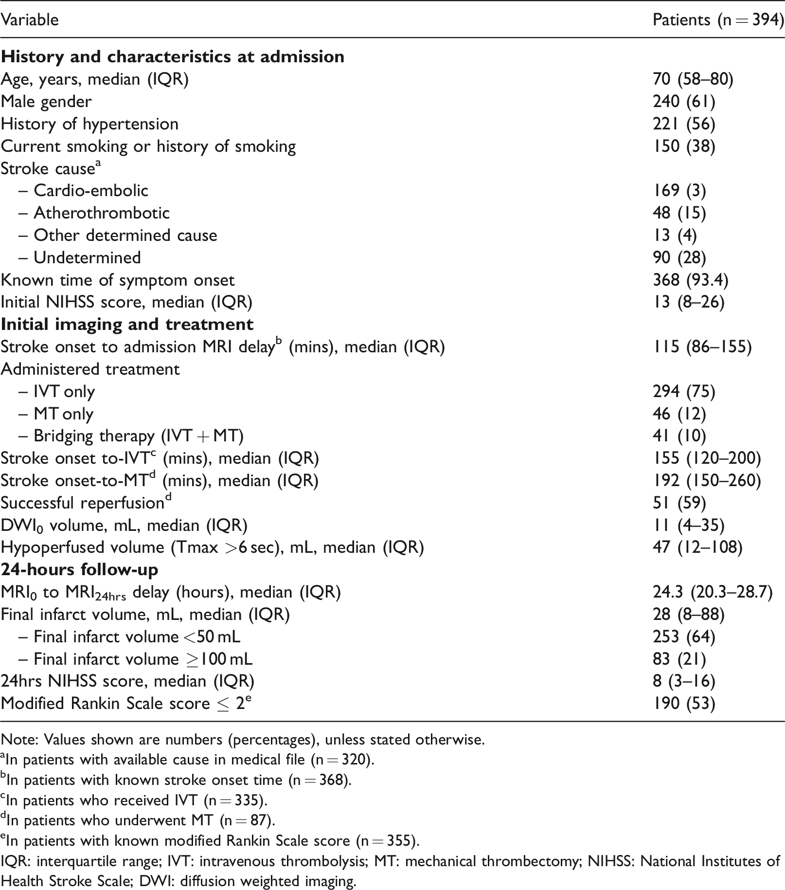
Note: Values shown are numbers (percentages), unless stated otherwise.

^aIn patients with available cause in medical file (n = 320).

^bIn patients with known stroke onset time (n = 368).

^cIn patients who received IVT (n = 335).

^dIn patients who underwent MT (n = 87).

^eIn patients with known modified Rankin Scale score (n = 355).

IQR: interquartile range; IVT: intravenous thrombolysis; MT: mechanical thrombectomy; NIHSS: National Institutes of Health Stroke Scale; DWI: diffusion weighted imaging.

Final infarct prediction performance

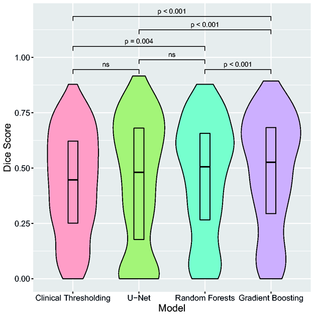
Gradient Boosting had significantly better Dice score as compared to all other models (P < 0.001), with a median score of 0.53 [IQR 0.29–0.68] (Table 2). Dice scores significantly differed among models, except between U-Net and Random Forests and between U-Net and clinical thresholding model (P = 0.13) (Figure 1). Using the AUC, AUC₀ and Mean Absolute Error, Gradient Boosting and U-Net performed equally well and outperformed Random Forests and clinical thresholding model (P < 0.001). There was no major overfitting for any of the studied models, as shown by the differences between Dice scores obtained in the training and test sets (Table 3). Dice scores were lower for volumes <50mL (0.44 [0.18–0.61] and 0.33 [0.03–0.58] for Gradient Boosting and U-Net, respectively; n = 253) than for volumes ≥100mL (0.70 [0.58–0.80] and 0.74 [0.60–0.80], respectively; n = 83). Adding other PWI maps as inputs did not modify model comparisons and none of the Extended-Perfusion models yielded significantly higher Dice scores than Tmax-only models (p > 0.1) (Table 3).

Table 2.

Final infarct prediction performance for each model.

Model	Dice score Median [IQR]	AUCMedian [IQR]	AUC₀Median [IQR]	Volume absolute error (mL) Mean±SD
Clinical thresholding	0.45 [0.25–0.62]	0.66 [0.61–0.72]	0.80 [0.7–0.86]	44.1 ± 56.0
U-Net	0.48 [0.18–0.68]	0.98 [0.95–0.99]	0.94 [0.88–0.97]	28.0 ± 37.8
Random forests	0.51 [0.27–0.66]	0.95 [0.90–0.98]	0.91 [0.85–0.95]	28.8 ± 42.2
Gradient boosting	0.53 [0.29–0.68]	0.98 [0.95–0.99]	0.94 [0.89–0.97]	27.7 ± 40.3

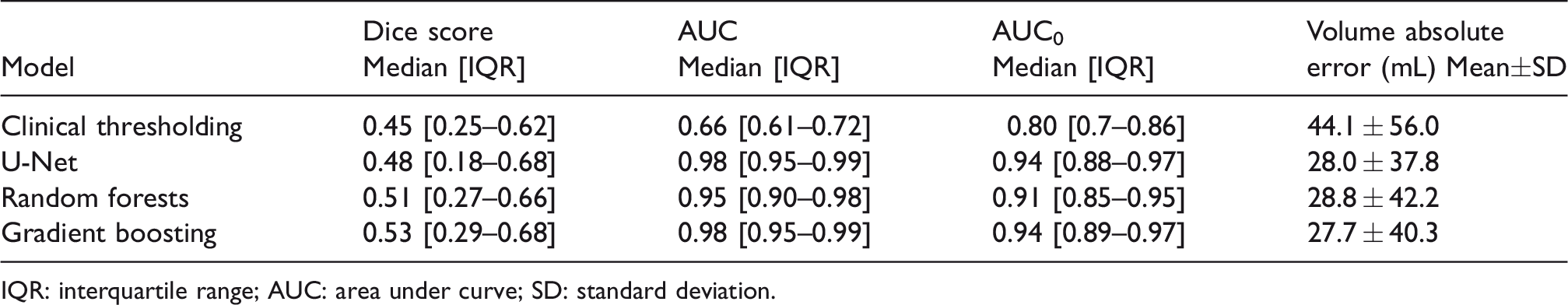
IQR: interquartile range; AUC: area under curve; SD: standard deviation.

Figure 1.

Final infarct volume prediction performance for each model.

Table 3.

Comparison of dice scores between training and test sets.

Models and inputs	Dice score in training setMedian [IQR]	Dice score in test setMedian [IQR]
Tmax-only models
U-Net	0.52 [0.24–0.69]	0.48 [0.18–0.68]
Random forests	0.58 [0.37–0.71]	0.51 [0.27–0.66]
Gradient boosting	0.57 [0.33–0.71]	0.53 [0.29–0.68]
Extended-perfusion models
U-Net	0.50 [0.19–0.69]	0.48 [0.17–0.68]
Random Forests	0.61 [0.42–0.73]	0.52 [0.28–0.67]
Gradient boosting	0.58 [0.37–0.71]	0.54 [0.31–0.68]

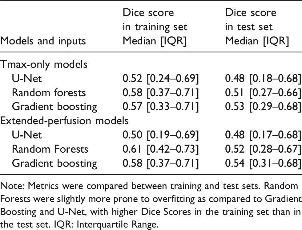
Note: Metrics were compared between training and test sets. Random Forests were slightly more prone to overfitting as compared to Gradient Boosting and U-Net, with higher Dice Scores in the training set than in the test set. IQR: Interquartile Range.

Reperfusion status

In the subgroup of patients treated with MT in which reperfusion data were available (n = 87), adding the reperfusion status as input significantly improved the performance of all models: Gradient Boosting (median Dice score 0.55 [IQR 0.28–0.64] vs. 0.47 [0.28–0.63], P = 0.008), Random Forests (0.48 [0.25–0.61] vs. 0.46 [0.23–0.61], P < 0.001), U-Net (0.46 [0.29-0.63] vs. 0.38 [0.12–0.55], P = 0.038), and clinical thresholding (0.49 [0.31–0.63] vs. 0.39 [0.22-0.59], P = 0.002).

Qualitative and quantitative assessment of final infarct volume

Illustrative examples of prediction maps are presented in Figure 2. By simple visual inspection, Random Forests and Gradient boosting yielded sharper and better contrasted but noisier prediction maps than U-Net. Bland-Altman analysis (illustrated only for Gradient Boosting and U-Net in Figure 3) demonstrated an underestimation of predicted volumes (mean difference: −18 mL [limits of agreement: −107-70mL] for Gradient Boosting and −14mL [−101-74mL] for U-Net), which was more prominent for larger volumes.

Figure 2.

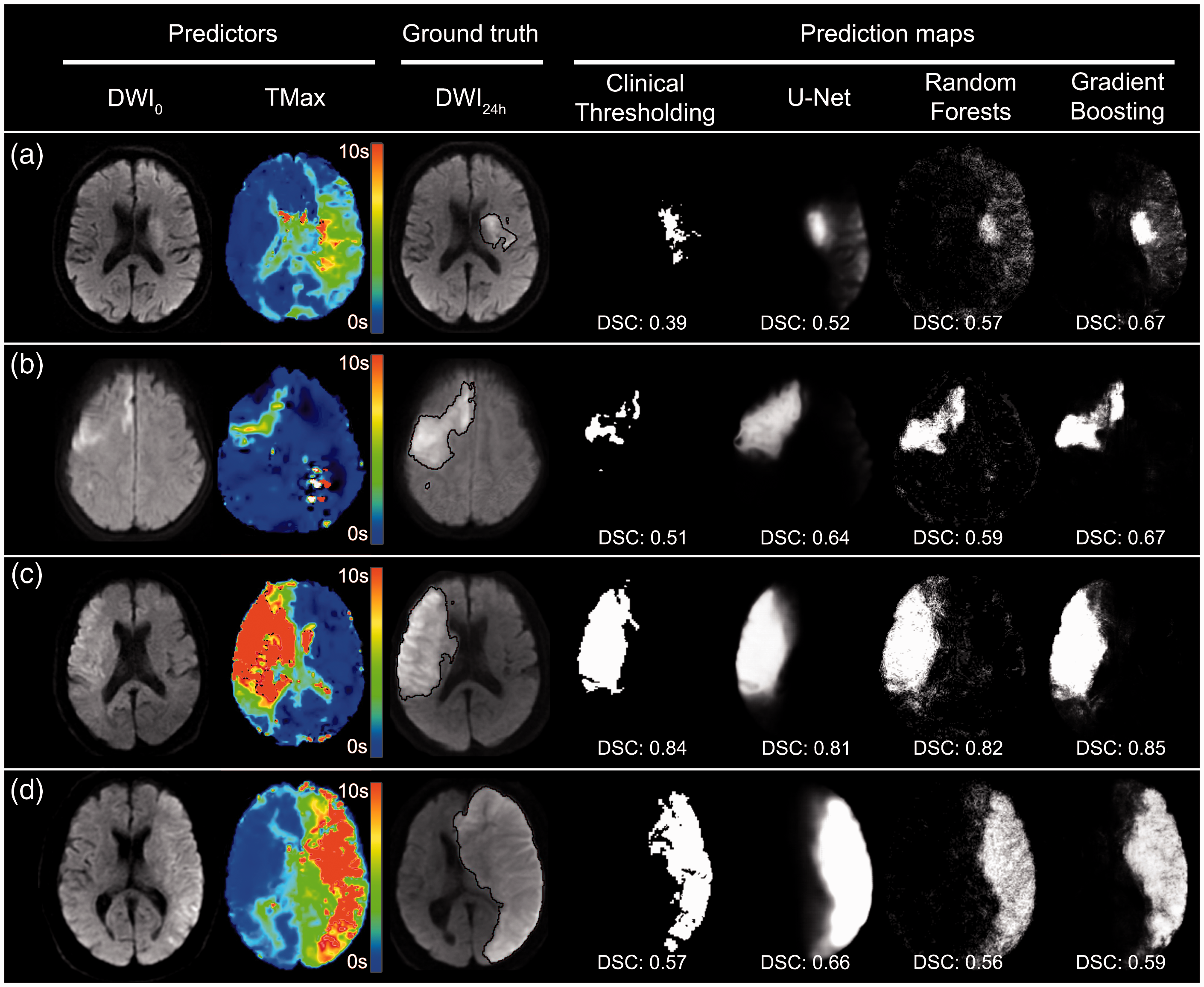
Examples of prediction maps with different models.

Figure 3.

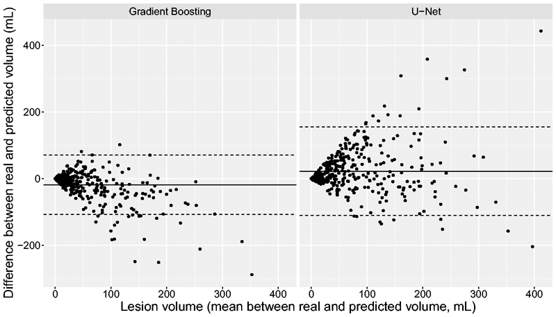
Bland-Altman plots for the Gradient Boosting and U-Net models.

Computation time

Training time was longer for U-Net (median duration per cross-validation fold: 160 minutes) than for Gradient Boosting (89 minutes) and Random Forests (19 minutes). Inference times for each patient were shorter for U-Net (median duration: 0.3 seconds) than for Gradient Boosting (21 seconds) and Random Forests (2 seconds).

Discussion

In this study, the three most popular ML segmentation models and the clinical thresholding method were compared for their performances in predicting final infarct, using a large single MRI dataset of AIS patients treated with reperfusion therapies. We found that Gradient Boosting model outperformed all other tested models including clinical thresholding method. Thus, Gradient Boosting produced better spatially defined and contrasted prediction maps, and accordingly would seem most suitable for clinical application. Of note, Gradient Boosting and U-Net yielded similar results with respect to absolute volume and AUC. Finally, all models tended to underestimate final infarct volume, especially for large infarcts.

Metrics analysis

Our results highlight the limitations of standard metrics for the evaluation of predictive models. The Dice score, which measures the overlap between predicted and ground-truth volumes, is theoretically the best metric to assess accuracy of both extent and spatial location of infarct prediction,³⁹ which are important determinants of stroke severity and long-term functional outcome.⁴⁰ Models with highest Dice score would thus best predict the fate of clinically relevant regions, although this metric in inherently unstable for small-size infarcts, as confirmed in our study.

Alternatively, AUC, although widely used, suffers from a large imbalance between (far more prevalent) healthy brain tissue and infarcted tissue. Hence, this metric carries limited information as all models reach very high AUC. The AUC₀, weighted on hypoperfused areas, is better adapted for small volumes and has the advantage of being threshold independent.¹ As for the AUC, it was markedly skewed to high values (between 0.89 and 0.98 across our models) and may as such afford lesser discrimination for model selection than Dice scores. Finally, Mean Absolute Error has the advantages of i) straightforward clinical significance given that infarct volume is known to correlate with clinical scores and outcome,⁴¹ and ii) invariance to spatial registration errors, but does not take into account spatial location errors.

Model comparisons

Overall, we obtained higher Dice scores than previously reported for both Random Forests¹⁵ or Gradient Boosting.¹⁷ This may be due to the fact that our models were trained and tested on large datasets with a wide range of infarct volumes, including larger ones (mean 60 mL ± 75 in our study vs 28 mL ± 79 in Grosser et al.,¹⁷ and median 28 mL in our study vs. 7.36 mL in McKinley et al.¹⁵). The overlap between predicted and real volume is indeed expected to increase with larger infarcts, irrespective of the model, as also shown here.

We found that Gradient Boosting outperformed Random Forests, in line with a recent study on 99 AIS patients.¹⁷ In this latter study, the difference in Dice scores between Gradient Boosting and Random Forests was comparable to ours (0.39 and 0.37 vs 0.53 and 0.51, respectively). This rather small gain in performance has to be put in balance with the additional computational cost, which in our study was 5 times longer with Gradient Boosting.

As compared with U-Net, Gradient Boosting had higher Dice score. This superiority might be due to differences in receptive fields between models. Patch-based models, such as Gradient boosting used here, have small receptive fields (patch: 5 × 5 voxels) as compared to U-Net (here, 32 × 32 voxels). Larger receptive fields should theoretically capture regional perfusion defects at a larger scale, and this may explain the better performance of U-Net for large infarct volumes. However, convolutional architectures use translation equivariance (i.e., the fact that the phenomenon of interest is equally likely to occur in all part of the image) as an inductive bias, which may be inadequate for AIS where lesions are not randomly localized but constrained by arterial territories. Moreover, U-Net prediction method did not outperform clinical thresholding model in our study. Although Deep Learning methods have been previously proposed in literature for tissue outcome prediction,¹⁸,¹⁹,³¹ it seems to outperform standard clinical thresholding methods in terms of Dice Score only in a patients with major reperfusion.³¹ It is however likely that the performance of Deep Learning methods, such as U-Net, being data-greedy, will continue to improve with access to very large amount of data whereas other ML approaches such as Gradient Boosting and Random Forests will tend to plateau despite access to the same amount of data.¹⁴ Future much larger multicentric datasets may thus be necessary to demonstrate the superiority of Deep Learning over other techniques. Beside its accuracy, the critical point for a clinically compatible software in AIS patients is the speed necessary to obtain prediction maps. Owing to their fast inference once trained, as shown in our study, Deep Learning models that do not require patch segmentation might better translate into clinically usable software.

The best performing models proposed in literature are presented in Table 4. Of note, all models outperformed linear models whenever compared.¹⁷,¹⁸,⁴²,⁴³ This was not unexpected since linear models combine linear transformations of voxel intensities and have limited expressive power. Accordingly, we chose to omit the comparison with linear models in our study.

Table 4.

Comparison with current literature.

Authors	Method^a	AUC	AUC₀	Dice Score	Mean volume absolute error (mL)	Number of patients (training/test set)
Scalzo et al.⁴²	Kernel spectral regression		0.91	–	–	25^b
Nielsen et al.¹⁸	Deep learning (SegNet)	–	0.88	–	–	187 (158/29)
McKinley et al.¹⁵	Random forests (FASTER)	–	–	0.34 (±0.22)	30 (±26)	100 (45/55)
Pinto et al.⁴⁷	Deep learning (U-Net + Gated recurrent unit)	–	–	0.35	–	75 (43/32)
Winder et al.⁴³	Random forests	–	–	0.45	–	90^b
Grosser et al.¹⁷	Gradient boosting		0.89	0.39	–	99^c
Yu et al.³¹	Deep learning (U–net)	0.92	–	0.53	–	182^d
Our study	Deep learning (U-Net)	0.98	0.94	0.48	28 (±38)	394^c
	Gradient boosting	0.98	0.94	0.53	27 (±40)	394^c

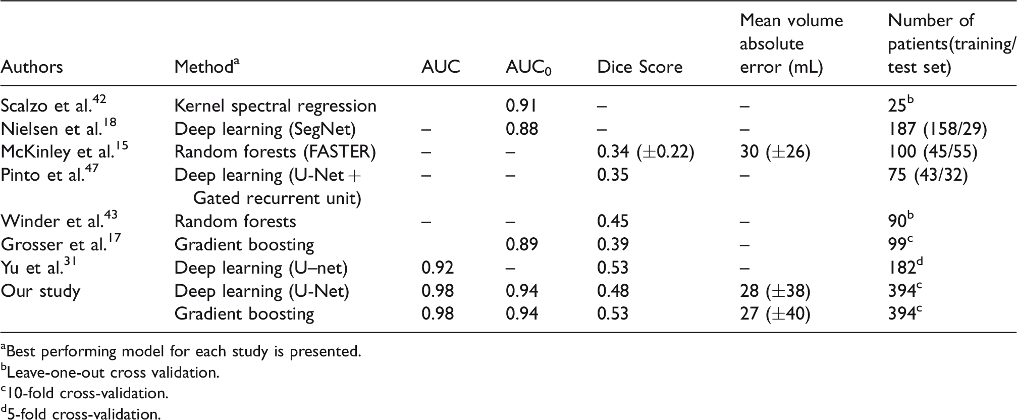
^aBest performing model for each study is presented.

^bLeave-one-out cross validation.

^c10-fold cross-validation.

^d5-fold cross-validation.

A recent large study reported better performance of a U-Net model than found in our study (Dice score: 0.53 vs 0.48, respectively).³¹ This could be explained by the use of a U-Net model with attention-gating units, which may improve U-Net performance. More likely, higher Dice score in this study are linked to larger final infarcts (median [IQR] 54 mL [16-117] vs. 28 mL [8-88] here) and more severe strokes that were imaged and treated later than in our study. Nielsen et al.¹⁸ have investigated another deep convolutional network (SegNet) for infarct prediction but obtained lower AUC₀ values (0.88 ± 0.12 vs. 0.94 for U-Net in our study). The ISLES 2016 and 2017 challenges compared many algorithms for final infarct prediction based on multimodal MRI in smaller populations (75 patients).²⁰ The best performing Deep Learning model yielded a lower Dice Score (0.32) than all the models tested in our study. However, these comparisons should be interpreted with caution given that population characteristics and sample size differ between studies. The raw metrics indeed appear highly dependent on the population studied, which emphasizes the importance of comparing concurrent models in the same sample. Although it is beyond the scope of the study to compare all existing models, we performed post-hoc supplementary analyses by comparing the performance of our U-Net model to the deep convolutional network proposed by Nielsen et al.¹⁸ on our data set. Performances were comparable, with similar median Dice scores (0.48 [0.19-0.66] for the network proposed by Nielsen et al vs. 0.48 [0.18-0.68] for our U-Net, P = 0.07). Other Deep Learning models, such as X-Net⁴⁴ or multi-path U-Net⁴⁵ have been proposed for acute AIS segmentation and may also be tested for prediction. Taking into account additional information regarding stroke texture might also be valuable.¹⁵ Furthermore, combining the results of different models with ensemble methods might boost the performances of individual models, as suggested in the ISLES 2017 challenge.²⁰

Patient heterogeneity and model interpretation

All ML models tested in this study underestimated true final infarct volume. This underestimation was more prominent for large infarcts, in line with a previous study of infarcts imaged in the subacute stage (3–7 days).³¹ Conversely, volume overestimations were observed in studies using ground truth infarct volume at later time points (1 month¹⁸ and 3 months¹⁵). These apparent discrepancies are likely explained by the natural evolution of necrotic lesions, which are characterized by peripheral vasogenic edema appearing ∼24hrs after stroke onset and peaking during the first week, followed by lesion shrinkage toward the chronic stage (1-3 months). Accordingly, volume underestimation observed in studies where ground truth is defined soon after treatment, including ours, likely reflects failure to capture vasogenic edema,³¹ while volume overestimation in studies with delayed ground truth reflects failure to capture lesion shrinkage.¹⁵,¹⁸

Reperfusion effect

Successful reperfusion is associated with limited infarct growth and better functional outcome.⁴⁶ As expected, integrating reperfusion status in our models improved their performance. This approach has been proposed in previous studies¹⁵,⁴⁷ using different frameworks. In the FASTER algorithm, McKinley et al. trained two separate models for reperfused and non-reperfused subjects.¹⁵ Pinto et al. integrated reperfusion status into their neural network using gated-recurrent unit.⁴⁷ We found a similar gain in performance (Dice score increment +0.07 here with Gradient boosting model vs. +0.05 in Pinto et al.⁴⁷) although we chose to concatenate reperfusion status with imaging data to ensure a similar architecture of all models for the sake of comparability. These results emphasize the potential clinical application of such prediction models. Indeed, for a given patient, creating differential prediction maps with and without reperfusion may have a direct application in treatment decision. Moreover, incorporation of other input parameters such as age, admission NIHSS, and glycaemia may improve prediction accuracy, although careful variable selection would be needed to limit model overfitting.

Limitations

Our study has limitations. First, we mainly focused on Tmax because of its known correlation with clinical outcome²⁷ and final infarct volume.⁴⁸ Moreover, it was the predominant contributing feature among other perfusion maps in a large ML study predicting tissue outcome in AIS.¹⁵ We however checked that Extended-Perfusion models did not outperform Tmax-only based models. One might consider other inputs, such as the CBF/Tmax ratio⁴⁹ which may be a marker of collateral status. An alternative approach entails the use of the source PWI images¹² instead of the parametric maps, which avoids the use of proprietary deconvolution software and integrates all information contained in the PWI dataset without the need for preliminary perfusion modeling. Second, our clinical thresholding model used predefined ADC and Tmax thresholds as done previously,³¹ although they are likely imperfect.^5–11 However, they represent the state-of-the-art for estimation of ischemic core and at-risk tissue, and are now used routinely in the clinical setting to select patient for MT beyond 6 hrs after stroke onset.⁴ Third, final infarct was defined on 24 hr follow-up MRI, an earlier time point than that used in previous studies.¹⁵,¹⁸ This approach was driven by consensus recommendations²⁸ and has the advantages of allowing more reliable segmentation thanks to the high natural contrast of infarcted tissue on DWI, of minimizing the risk of final infarct overestimation due to vasogenic edema that peaks around day 3-5²⁸ and of reducing the odds of both early stroke recurrence and drop-outs. Fourth, we limited our analysis to the effect of reperfusion status in the subgroup of patients who underwent MT, since documentable early reperfusion status was not available in patients treated with IVT only. Fifth, binary outcome prediction maps were generated using an arbitrary fixed threshold (0.5) applied on ML probability maps. However, Dice scores were not significantly improved using a threshold optimization method (see Online-Only Data Supplement, Supplemental Table 1). Sixth, we used a cross-validation scheme, which increases the statistical power but reduces the interpretability of trained models. In order to check the robustness of our findings, we conducted an additional analysis using a single train/validation/test split with a larger test set (25%). Results were similar in terms of Dice scores (see Online-Only Data Supplement, Supplemental Table 2) but statistical power was insufficient to conclude regarding differences between ML models (e.g. 0.54 for Gradient Boosting vs. 0.52 for U-Net, P = 0.06) (see Online-Only Data Supplement, Supplemental Figure 1). Finally, this was a single-center study, and all patients had a standardized stroke MR protocol. While this increases data homogeneity and hence model performance, the trained models may not perform equally well on a more heterogeneous multi-center dataset.

Conclusion

The present work reports a benchmark of ML models for tissue outcome prediction in acute stroke using a large dataset. All models outperformed the thresholding PWI-DWI methods used in clinical practice. Among the three ML models, Gradient Boosting appeared particularly relevant for predicting tissue fate after AIS, followed closely by Random Forests and U-Net. These novel approaches appear promising for predicting tissue outcome and hence decision-making.

Supplemental Material

sj-pdf-1-jcb-10.1177_0271678X211024371 - Supplemental material for Tissue outcome prediction in hyperacute ischemic stroke: Comparison of machine learning models

Supplemental material, sj-pdf-1-jcb-10.1177_0271678X211024371 for Tissue outcome prediction in hyperacute ischemic stroke: Comparison of machine learning models by Joseph Benzakoun, Sylvain Charron, Guillaume Turc, Wagih Ben Hassen, Laurence Legrand, Grégoire Boulouis, Olivier Naggara, Jean-Claude Baron, Bertrand Thirion and Catherine Oppenheim in Journal of Cerebral Blood Flow & Metabolism

Footnotes

Funding

The author(s) received no financial support for the research, authorship, and/or publication of this article.

Acknowledgements

Not applicable.

Declaration of conflicting interests

The author(s) declared no potential conflicts of interest with respect to the research, authorship, and/or publication of this article.

Authors’ contributions

JB made a substantial contribution to the concept and design of the study, acquisition and analysis of the data, drafted the article and approved the version to be published

WBH made a substantial contribution to the concept of the study and acquisition of data, revised critically the article and approved the version to be published

SC, GT, LL, GB and ON made a substantial contribution to the concept and design of the study, revised critically the article and approved the version to be published

JCB made a substantial contribution to the concept of the study and data analysis, revised critically the article and approved the version to be published

BT and CO made a substantial contribution to the concept and design of the study, analysis and interpretation of data, revised critically the article and approved the version to be published

ORCID iDs

Joseph Benzakoun

Wagih Ben Hassen

Supplemental material

Supplemental material for this article is available online.

References

Jonsdottir

Østergaard

Mouridsen

Predicting tissue outcome from acute stroke magnetic resonance imaging: improving model performance by optimal sampling of training data. Stroke 2009; 40: 3006–3011.

Kidwell

Wintermark

De Silva

, et al. Multiparametric MRI and CT models of infarct core and favorable penumbral imaging patterns in acute ischemic stroke. Stroke 2013; 44: 73–79.

Albers

Goyal

Jahan

, et al. Ischemic core and hypoperfusion volumes predict infarct size in SWIFT PRIME. Ann Neurol 2016; 79: 76–89.

Albers

Marks

Kemp

, et al. Thrombectomy for stroke at 6 to 16 hours with selection by perfusion imaging. N Engl J Med 2018; 378: 708–718.

Oppenheim

Grandin

Samson

, et al. Is there an apparent diffusion coefficient threshold in predicting tissue viability in hyperacute stroke? Stroke 2001; 32: 2486–2491.

Purushotham

Campbell

BCV

Straka

, et al. Apparent diffusion coefficient threshold for delineation of ischemic core. Int J Stroke 2015; 10: 348–353.

Thomas

RGR

Lymer

Armitage

, et al. Apparent diffusion coefficient thresholds and diffusion lesion volume in acute stroke. J Stroke Cerebrovasc Dis 2013; 22: 906–909.

Olivot

J-M

Mlynash

Thijs

, et al. Optimal Tmax threshold for predicting penumbral tissue in acute stroke. Stroke 2009; 40: 469–475.

Takasawa

Jones

Guadagno

, et al. How reliable is perfusion MR in acute stroke? Validation and determination of the penumbra threshold against quantitative PET. Stroke 2008; 39: 870–877.

10.

d’Esterre

Boesen

Ahn

, et al. Time-dependent computed tomographic perfusion thresholds for patients with acute ischemic stroke. Stroke 2015; 46: 3390–3397.

11.

Bandera

Botteri

Minelli

, et al. Cerebral blood flow threshold of ischemic penumbra and infarct core in acute ischemic stroke: a systematic review. Stroke 2006; 37: 1334–1339.

12.

Scalzo

Sarma

, et al. Predicting ischemic stroke tissue fate using a deep convolutional neural network on source magnetic resonance perfusion images. J Med Imag 2019; 6: 1.

13.

Tisserand

Malherbe

Turc

, et al. Is white matter more prone to diffusion lesion reversal after thrombolysis? Stroke 2014; 45: 1167–1169.

14.

Mouridsen

Thurner

Zaharchuk

Artificial intelligence applications in stroke. Stroke 2020; 51: 2573–2579.

15.

McKinley

Häni

Gralla

, et al. Fully automated stroke tissue estimation using random forest classifiers (FASTER). J Cereb Blood Flow Metab 2017; 37: 2728–2741.

16.

Maier

Handels

, et al. Predicting stroke lesion and clinical outcome with random forests. In: Crimi

Menze

Maier

(eds) Medical image computing and computer assisted intervention: BrainLes. Athens, Greece: Springer International Publishing, 2016; 10154: 219–230.

17.

Grosser

Gellißen

Borchert

, et al. Improved multi-parametric prediction of tissue outcome in acute ischemic stroke patients using spatial features. PLoS ONE 2020; 15: e0228113.

18.

Nielsen

Hansen

Tietze

, et al. Prediction of tissue outcome and assessment of treatment effect in acute ischemic stroke using deep learning. Stroke 2018; 49: 1394–1401.

19.

Stier

Vincent

Liebeskind

, et al. Deep learning of tissue fate features in acute ischemic stroke. Proceedings (IEEE Int Conf Bioinformatics Biomed) 2015; 2015: 1316–1321.

20.

Winzeck

Hakim

McKinley

, et al. ISLES 2016 and 2017-benchmarking ischemic stroke lesion outcome prediction based on multispectral MRI. Front Neurol 2018; 9: 679.

21.

Yang

Lei

Shu

H-K

, et al. Pseudo CT estimation from MRI using patch-based random forest. Proc SPIE Int Soc Opt Eng 2017; 10133: 101332Q.

22.

Accident Vasculaire Cérébral (AVC). Haute Autorité de Santé, www.has-sante.fr/jcms/p_3058302/fr/accident-vasculaire-cerebral-avc (accessed 22 May 2020).

23.

Jenkinson

Bannister

Brady

, et al. Improved optimization for the robust and accurate linear registration and motion correction of brain images. Neuroimage 2002; 17: 825–841.

24.

Jenkinson

Smith

A global optimisation method for robust affine registration of brain images. Med Image Anal 2001; 5: 143–156.

25.

Østergaard

Weisskoff

, et al. Tracer arrival timing-insensitive technique for estimating flow in MR perfusion-weighted imaging using singular value decomposition with a block-circulant deconvolution matrix. Magn Reson Med 2003; 50: 164–174.

26.

Mouridsen

Christensen

Gyldensted

, et al. Automatic selection of arterial input function using cluster analysis. Magn Reson Med 2006; 55: 524–531.

27.

Seker

Pfaff

Potreck

, et al. Correlation of Tmax volumes with clinical outcome in anterior circulation stroke. Brain Behav 2017; 7: e00772.

28.

Warach

Luby

Albers

, et al.; Stroke Imaging Research (STIR) and VISTA-Imaging Investigators. Acute stroke imaging research roadmap III. Stroke 2016; 47: 1389–1398.

29.

Luby

Bykowski

Schellinger

, et al. Intra- and interrater reliability of ischemic lesion volume measurements on diffusion-weighted, mean transit time and fluid-attenuated inversion recovery MRI. Stroke 2006; 37: 2951–2956.

30.

Soize

Tisserand

Charron

, et al. How sustained is 24-hour diffusion-weighted imaging lesion reversal? Serial magnetic resonance imaging in a patient cohort thrombolyzed within 4.5 hours of stroke onset. Stroke 2015; 46: 704–710.

31.

Xie

Thamm

, et al. Use of deep learning to predict final ischemic stroke lesions from initial magnetic resonance imaging. JAMA Netw Open 2020; 3: e200772.

32.

Arlot

Celisse

A survey of cross-validation procedures for model selection. Statist Surv 2010. 4: 40–79.

33.

Gençay

Pricing and hedging derivative securities with neural networks: Bayesian regularization, early stopping, and bagging. IEEE Trans Neural Netw 2001; 12: 726–734.

34.

Zaidat

Yoo

Khatri

, et al.; STIR Thrombolysis in Cerebral Infarction (TICI) Task Force. Recommendations on angiographic revascularization grading standards for acute ischemic stroke: a consensus statement. Stroke 2013; 44: 2650–2663.

35.

Oppenheim

Samson

Manaï

, et al. Prediction of malignant middle cerebral artery infarction by diffusion-weighted imaging. Stroke 2000; 31: 2175–2181.

36.

de Margerie-Mellon

Turc

Tisserand

, et al. Can DWI-ASPECTS substitute for lesion volume in acute stroke? Stroke 2013; 44: 3565–3567.

37.

Wickham

ggplot2: elegant graphics for data analysis. New York, NY: Springer-Verlag, 2016.

38.

Lehnert

BlandAltmanLeh: Plots (Slightly Extended) Bland-Altman Plots, https://CRAN.R-project.org/package=BlandAltmanLeh (2015, accessed 4 June 2020).

39.

Zou

Warfield

Bharatha

, et al. Statistical validation of image segmentation quality based on a spatial overlap index. Acad Radiol 2004; 11: 178–189.

40.

Cloonan

Mocking

SJT

, et al. The role of acute lesion topography in initial ischemic stroke severity and long-term functional outcomes. Stroke 2015; 46: 2438–2444.

41.

Yaghi

Herber

Boehme

, et al. The association between diffusion MRI-defined infarct volume and NIHSS score in patients with minor acute stroke. J Neuroimaging 2017; 27: 388–391.

42.

Scalzo

Hao

Alger

, et al. Regional prediction of tissue fate in acute ischemic stroke. Ann Biomed Eng 2012; 40: 2177–2187.

43.

Winder

Siemonsen

Flottmann

, et al. Technical considerations of multi-parametric tissue outcome prediction methods in acute ischemic stroke patients. Sci Rep 2019; 9: 13208.

44.

Yang

, et al. X-Net: brain stroke lesion segmentation based on depthwise separable convolution and long-range dependencies. In: Proceedings, Part III medical image computing and computer assisted intervention, Shenzhen, China: Springer International Publishing, 2019, pp. 247–255.

45.

Dolz

Ben

Desrosiers

, et al. Dense multi-path U-Net for ischemic stroke lesion segmentation in multiple image modalities. In: Crimi

Bakas

Kuijf

(eds) BrainLes (Revised selected papers, part I). Granada, Spain: Springer International Publishing, 2018, pp.271–282.

46.

Marks

Lansberg

Mlynash

, et al.; for the DEFUSE Investigators. Angiographic outcome of endovascular stroke therapy correlated with MR findings, infarct growth, and clinical outcome in the DEFUSE 2 trial. Int J Stroke 2014; 9: 860–865.

47.

Pinto

McKinley

Alves

, et al. Stroke lesion outcome prediction based on MRI imaging combined with clinical information. Front Neurol 2018; 9: 1060.

48.

Shih

Saver

Alger

, et al. Perfusion-weighted magnetic resonance imaging thresholds identifying core, irreversibly infarcted tissue. Stroke 2003; 34: 1425–1430.

49.

Galinovic

Kochova

Khalil

, et al. The ratio between cerebral blood flow and Tmax predicts the quality of collaterals in acute ischemic stroke. PLoS One 2018; 13: e0190811.

Supplementary Material

Please find the following supplemental material available below.

For Open Access articles published under a Creative Commons License, all supplemental material carries the same license as the article it is associated with.

For non-Open Access articles published, all supplemental material carries a non-exclusive license, and permission requests for re-use of supplemental material or any part of supplemental material shall be sent directly to the copyright owner as specified in the copyright notice associated with the article.

0.00 MB

0.85 MB