Sage Journals: Discover world-class research

Abstract

The business models for the operation of battery storage systems often depend substantially upon the revenues from arbitrage in the daily electricity wholesale market. Other revenue streams can be attractive, but even with them, wholesale market arbitrage is often used as the benchmark. There can be various trading policies for wholesale market arbitrage and this paper provides a comparison of three main variations. These are: day-ahead spread trading, day-ahead trading with look-ahead and intra-day continuously trading with look-ahead. The example is from the GB electricity market in which wind and solar generation as well as demand forecasts are used to forecast electricity prices. The results of the back-testing indicate the comparative attractiveness of day-ahead spread trading in terms of risk and return performance.

JEL Classification: Q28

Keywords

electricity batteries spreads trading

1. Introduction

Whilst it is clear that the motivation for the widespread deployment of batteries in electricity markets has been a technological one, as a response to the highly intermittent production of power from renewable resources such as wind and solar, the profitable business models to support their merchant operations depend essentially upon price spreads in the various markets which they can access. The widespread introduction of renewable technologies such as wind and solar has increased the volatility of market prices and thus the opportunities for battery owners to profit from arbitrage trading have also increased.

Within day-ahead wholesale electricity markets, the spread between night-time price troughs and day-time price peaks has been, for many years, the rationale for hydro-pumped storage operating a daily cycle. However, with the influx of solar generation there may be another trough in demand on the system, and therefore price, at midday. With battery operations having a more efficient energy cycle than pumped storage, it can therefore often be profitable for them to operate on two cycles per day (as indicated in Abramova and Bunn 2021). However, distinct from intraday price spreads, inter-day price spreads may also offer arbitrage opportunities, and so the question of whether the optimal operation should have a daily horizon or longer is material. Furthermore, whether the traders should seek pure arbitrage positions in which their buy and sell positions are closed (pure spreads) or open set-point strategies, in which the battery is charged or discharged according to a continuous policy regarding the dynamics of the price level, is a further consideration. Various operational policies have been advocated by researchers and much depends upon the dynamic microstructure of the markets. In addition, there are spreads between the various markets for short-term reserves (as required by the transmission and distribution network system operators) and the wholesale market, thereby offering the possibility to sell reserve power to the system operators having charged more cheaply from the wholesale market.

In this research we seek to compare the main wholesale arbitrage trading policies building upon the body of previous research. For example, Abramova and Bunn (2020) developed accurate forecasting models for the densities of hourly spreads from the day-ahead auction in Germany and have shown from backtesting how arbitrage trading of these spreads can be profitable with minimal risk. Similarly, whilst energy storage systems can get paid from a variety of ancillary services such as spinning reserve (Marchgraber et al. 2020) and frequency control (Delille, Francois and Malarange 2012), the wholesale market arbitrage has remained the main source of revenue (Staffell and Rustomji 2016). The attraction of pure day-ahead spread trading has been based upon the closed positions, once acquired, being risk-free, supporting the day-ahead operational planning. We refer to this as episodic since the day-ahead auction typically clears once a day providing a vector of prices for all the hours of the following day. A wide diversity of these episodic daily arbitrage cycles has been reported including Foster (2017) who describes its operation at the Tesla installation in Australia and Mohsenian-Rad (2015), Salles et al. (2016), Lucas (2019) who document applications in California, PJM, and London respectively. Núñez, Canca and Arcos-Vargas (2022) provide a broad comparison of arbitrage profitability across European countries, using a detailed optimization model on 2019 data. They suggest that whilst arbitrage profits alone may not have been sufficient to support capital investments in Li-Ion batteries in 2019, they will do so in the future as price spreads become larger (a conclusion also advanced by LCP 2021). In contrast, some research has also focused on advances in battery technology on the arbitrage economics (eg. Arcos-Vargas, Canca and Núñez 2020; Daggett, Qadrdan and Jenkins 2017).

This episodic day-ahead arbitrage is in contrast to a continuous process of trading with open positions activated closer to real-time. Continuous storage policies for gas and hydro have an extensive history of developments but have been less adapted to electricity, mainly because of the attraction of the episodic, repeated daily cycles of distinct arbitrage opportunities. However, Jiang and Powell (2015) developed a continuous approach using approximate dynamic programming for optimal one-hour-ahead bidding by energy storage operators in real-time electricity markets and this was extended to deal with risk aversion in Jiang and Powell (2017). Elsewhere, Juárez and Musilek (2021) simulated two battery technologies, lithium-ion and vanadium redox flow, in the context of real-time continuous operation, whilst, Shu and Jirutitijaroen (2013) developed a continuous decision model for a battery linked to a wind generation facility. The continuous trading research focus has tended to be on the optimization techniques, for example, in the application of Xi, Sioshansi and Marano (2014), the main research contribution was in the stochastic dynamic programming formulation. A partial compromise between the day-ahead episodic trading and the continuous real-time policies is provided by the episodic look-ahead approach which takes into account the provisional decisions on subsequent day(s) in the day-ahead trading model. This has been used by Wang et al. (2017) and Aliasghari, Zamani-Gargari and Mohammadi-Ivatloo (2018). Notwithstanding these examples of different trading approaches, comparisons across these different approaches with real backtesting appear to be absent from empirical research.

Thus, we compare the day-ahead spread trading, with and without look-ahead, with continuous trading, also with look-ahead, using a sample of GB electricity market data. Multi-factor price forecasting models are used to estimate day-ahead auction prices (DAP) and the close-to-real-time intraday market prices. Optimal ex ante trading decisions are back-tested using the realized electricity prices. From a research perspective, a priori, it is not obvious which method should perform best. The episodic spread trading from the day-ahead auction locks-in the profit day ahead and thereby appears to involve less risk and possibly lower transaction costs than a sequence of open positions with continuous intraday trading. However, it does require price forecasts to be made prior to the auction so that the battery operator knows which delivery periods to target for the offer(s) and bid(s) corresponding to potential discharging and charging. Furthermore, a pure spread trading policy that closes the spread position within a day means that the opening and closing state of charge of the battery should be the same day by day. A look-ahead strategy can relax that constraint but requires accurate forecasts over the longer horizon. Likewise, whilst continuous trading can, in one sense, be more accurate by taking open positions closer to real-time, it still needs to undertake this in the light of forecasts for future intraday prices over a planning horizon. Moreover, the dynamics of intraday prices will be different from those of the day-ahead auctions, such that one or the other may offer greater temporal arbitrage returns based upon their predictable time series variations.

The remainder of this paper is organized as follows. The description of the problem and the mathematical formulation are set out in Section 2. In Section 3 the data and forecasting model are described. Then, the results of the daily optimizations of each strategy and the backtesting results are presented. The final sections present a discussion and conclusions.

2. Formulations

In this section, we characterize and model the three different arbitrage trading strategies. The batteries are considered to be sufficiently small so as not to influence prices and flexible enough to charge or discharge within an hour. Under these conditions the initial level of the battery at the start of each day will either be 1 (full) or 0 (empty). It is easy to show that for the arbitrage decisions in this setting, intermediate opening charge levels would be suboptimal. During the charging and discharging process, there will be a power loss which we denote by an efficiency parameter. A transaction cost will also be applicable for each electricity trade, covering system as well as market fees, and these of course vary from market to market and possibly also by time of day and location. We consider an arbitrary transaction cost.

2.1. Day-Ahead Trading With and Without Look-Ahead

For the day-ahead market, market participants are presumed to submit bids and offers for each hour of the next day before 12:00 noon. The day-ahead market will be closed and cleared at 12:00 noon and will yield the day-ahead prices (DAP_t) for all twenty-four hours of the following day. A spread trade can be regarded as a special day-ahead trade, based on the price spread between two different hours of the day. In spread trading from the day-ahead auction, a reversal of a position will be executed at the same time, buy and then sell on the next day, or sell and then buy on the next day. The most important consequence of this spread trade, more specifically a fully balanced spread trade, is that the initial and final levels of the battery will necessarily be the same each day, either 1 or 0. There could be opportunities for multiple pairs of buy and sell and/or sell and buy operations in a day, as in Abramova and Bunn (2021).

Departing from the fully balanced spread trade for a single day ahead, the look-ahead variation seeks to optimize with forecasts over two successive days and thereby potentially obtain the optimal state of the last hour of day 1, in view of what might be traded on day 2. In our formulation, to support this, the battery operators predict day-ahead auction prices for day 1 and day 2 before noon on day 0. Based on the predicted prices on these two days, the battery operator makes a firm decision for the day1 battery operation and bids into the day-ahead auction accordingly. The plan for day 2 is necessarily provisional (there is no auction for two days ahead) and its expected valuation is discounted, as in Wang et al. 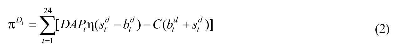(2017) by the factor $α^{D_{2}}$ . The planning window then rolls forward a day. The discrete daily steps in the time series are indexed by the variable d. The predicted prices for day 2 and day 3 are then used to determine the operation of Day 2, and so on.

Equations (1) to (9) specify the day-ahead trade model with look-ahead. All variables and parameters are defined in the nomenclature table in the Appendix. The day-ahead trading with no look-ahead is a simple restricted version of this model. The operational profit contribution, maximized over an optimization window of two days, is therefore specified as:

\max π^{d} = π^{D_{1}} + α^{D_{2}} π^{D_{2}}

(1)

The operational profit contribution for day1 or day2 is the sum of the revenue or cost of selling (s) or buying (b) electricity for each hour of the day minus the cost incurred by the transaction, C(.), as in equations (2) and (3) respectively. The index t denotes the hour in each day; whilst d is the index for each day. During the charging and discharging of the battery, there is a loss of power and so an efficiency term η is introduced.

π^{D_{1}} = \sum_{t = 1}^{24} [D A P_{t} η (s_{t}^{d} - b_{t}^{d}) - C (b_{t}^{d} + s_{t}^{d})]

(2)

π^{D_{2}} = \sum_{t = 25}^{48} [D A P_{t} η (s_{t}^{d} - b_{t}^{d}) - C (b_{t}^{d} + s_{t}^{d})]

(3)

Equations (4) and (5) constrain the battery to only be charged or discharged each hour using a binary variable. In Abramova and Bunn (2021) it was proven that partial utilization of battery capacity would be suboptimal in hourly trading with batteries able to fully charge or discharge within an hour. Thus:

0 \leq b_{t}^{d} \leq 1 - x_{t}^{d} \forall_{t}

(4)

0 \leq s_{t}^{d} \leq x_{t}^{d}

(5)

x_{t}^{d} \in {0, 1} \forall_{t}

(6)

The dynamics of the battery charge level ( $S o C_{t}^{d}$ ) are represented by equations (7) and (8), starting from the initial opening state, $S o C_{0}^{d}$ . Equation (9) constrains the upper and lower limits of the battery level.

S o C_{t}^{d} = S o C_{0}^{d} + b_{t}^{d} - s_{t}^{d} \forall t = 1

(7)

S o C_{t + 1}^{d} = S o C_{t}^{d} + b_{t}^{d} - s_{t}^{d} \forall 1 < t \leq 48

(8)

S o C_{\min} \leq S o C_{t}^{d} \leq S o C_{\max} \forall t

(9)

2.2. Continuous Trading With Look-Ahead

Continuous trading is formulated here on the basis of the latest intraday market price before delivery. We use the Market Index Price (MIP_t) from Elexon, being a weighted average of the intraday trading prices for a particular delivery period t predominantly based upon trades within the final hour before delivery (Elexon 2021). In contrast to the episodic day-ahead trading, the model of continuous trading has decisions being made every hour. For notation, therefore, we no longer focus upon a time series of days, d, but on time series of hours, indexed by t. In the previous case of daily episodic trading, t designated the hour in a particular day, d. In this continuous case, t runs throughout the whole time series without regard to the actual days involved. As in the episodic look-ahead framework, each hourly decision at t is made in the light of a provisional plan over a subsequent planning window of length $t - 8760$ .

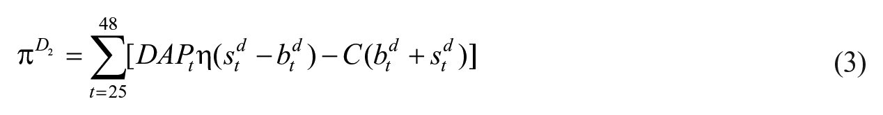
The continuous formulation is represented by equations (10) to (16). The objective function, shown in equation (10), is the sum of the revenues over the future look-ahead window.

π^{c} = \sum_{t = 1}^{T^{'}} [M I P_{t} η (s_{t}^{c} - b_{t}^{c}) - C (b_{t}^{c} + s_{t}^{c})]

(10)

Charging and discharging of the battery for each hour of operation is restricted by equations (11) to (13).

0 \leq b_{t}^{c} \leq 1 - x_{t}^{c} \forall t

(11)

0 \leq s_{t}^{c} \leq x_{t}^{c} \forall t

(12)

x_{t}^{c} \in {0, 1} \forall t

(13)

Equations (14) to (16) show the evolution of the battery charge level at each hour from the opening, initial state.

S o C_{t}^{c} = S o C_{0}^{c} + b_{t}^{c} - s_{t}^{c} \forall t = 1

(14)

S o C_{t + 1}^{c} = S o C_{t}^{c} + b_{t}^{c} - s_{t}^{c} \forall 1 < t \leq T^{'}

(15)

S o C_{\min} \leq S o C_{t}^{c} \leq S o C_{\max} \forall t

(16)

3. Data and Forecasts

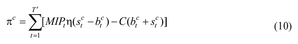
All data come from the GB electricity market. For the day-ahead trading with and without look-ahead we took the day-ahead auction prices (DAP) from N2EX, which is the trading platform established by NordPool in partnership with NASDAQ OMX. For the continuous intraday data we used the Market Index Price (MIP) from Elexon which reflects the prices from trades for to two hours before delivery (Elexon 2021). The day-ahead auction prices are available in hourly and half-hourly versions. We chose the hourly prices because of its higher liquidity and to fit better into the battery optimization model. For the MIP, we averaged the two half-hourly prices to be comparable. Figure 1 displays the average hourly DAP and MIP prices for 2019 to 2021. The DAP exhibits greater hourly variation across the day with an overall standard deviation of 71.46 compared to the MIP’s 63.65.

Figure 1.

Daily averaged DAP and MIP from 2019 to 2021.

Spreads are what drive battery operators to undertake arbitrage trades. We have calculated the 276 possible spreads for DAP and MIP for each day and Table 1 shows their descriptive statistics. We see that the mean spread is larger for DAP than that for MIP if the trades are both completed in one day, while the DAP spreads have higher variance. This means that under DAP the battery operators may have more potential for profitable arbitrage trades.

Table 1.

The Statistics Description for DAP Spreads and MIP Spreads From 2019 to 2021.

	DAPSpread	MIPSpread
Mean	10.6317	8.41492
Standard deviation	62.2142	46.7996
Min	−2,374.9	−1,762.4
25%	−3.01	−3.525
50%	5.26	4.165
75%	15.88	14.65
Max	2,386.94	1,796.83

3.1. Forecasting the DAP

As with many applications in the research literature on electricity day-ahead price forecasting, we developed a linear econometric forecasting approach that included the typical predictive variables that market participants would consider: (1) lagged day-ahead electricity prices, (2) day-ahead wind generation forecasts, (3) day-ahead solar power forecasts, (4) day-ahead load forecast, (5) forward daily gas price, (6) forward daily coal price, and (7) day-ahead reserve margin forecast (de-rated for average availabilities), “DRM.” All predictive variables are available day ahead and we have chosen to use a relatively straightforward regression model to reflect what might be used in practice. The day ahead forecasts are available on an hourly basis, whilst the day ahead commodity prices for gas and coal are daily. For looking further ahead than one day, only the lagged one-day-ahead predictors can be used as two-day-ahead forecasts were not available. Descriptive statistics for these variables, including cross correlations, are included in the Appendix.

The purpose of this research is not to develop new price forecasting methods but to understand the relative benefits of day ahead and continuous arbitrage trading. We therefore need to have a consistent approach to prediction in both cases. The day ahead prices are stationary (ADF test statistics of −7.7 and −5.9 for MIP and DAP strongly rejected unit roots) and so price levels could be used without differencing. The regression model to predict DAP_d,t, the day ahead price for each hour t of each day d, is specified as follows:

D A P_{d, t} = α + β_{1} D A P_{d - 1, t} + β_{2} D R M_{d, t} + β_{3} G a s_{d, t} + β_{4} C o a l_{d, t} + β_{5} e_{d, t}

(17)

e_{d, t} = L o a d_{d, t} - W i n d_{d, t} - S o l a r_{d, t}

(18)

Similarly, the forecasting model for two-day-ahead auction price is as follows:

D A P_{d, t} = α + β_{1} D A P_{d - 2, t} + β_{2} D R M_{d - 1, t} + β_{3} G a s_{d - 1, t} + β_{4} C o a l_{d - 1, t} + β_{5} e_{d - 1, t}

(19)

e_{d - 1, t} = L o a d_{d - 1, t} - W i n d_{d - 1, t} - S o l a r_{d - 1, t}

(20)

All coefficients were significant and the regression residuals were adequately specified with respect to serial correlation (DW statistic around 1.7 in both case was acceptable). There was no need to include further lags and seasonality was captured by the exogenous predictors, as in Karakatsani and Bunn (2008).

Data are taken for GB, 2019 to 2021. The electricity market price data are sourced from NordPool. Wind forecasts, solar forecasts, load forecasts, and DRM forecasts are sourced from the Balancing Mechanism Reporting Service (BMRS) (Elexon 2024). The gas prices (one price/day) refer to NBP and the coal price (one price/day), using the ARA marker, are sourced from Bloomberg. Missing coal and gas prices from the weekends are interpolated. We use a rolling 365-day window for estimation meaning that forecasts of the day-ahead auction prices for a particular day and the next are based on a model estimated from the previous 365 days. We make decisions using predicted day-ahead prices and back-test out-of-sample using the real electricity prices. The error statistics for the forecasting model are shown in Table 2. The R-squared statistic compares the forecast electricity prices with the actual outcomes.

Table 2.

The Day-ahead Forecast Error Statistics.

	Day-ahead forecast	Two-day-ahead forecast
Mean	0.246	2.020
Std Dev	47.957	55.116
R-squared	0.698	0.610

Because robustness to forecasting accuracy is an issue, we consider the sensitivity of our trading results to the use of a less accurate predictor and a perfect predictor (described later).

3.2. Forecasting the MIP

We assume that hourly MIP forecasts will update the DAP prices for each hour adaptively throughout the following day. Thus, the predictions for MIP rely on the prediction of errors between MIP and DAP, derived from (1) the difference between day-ahead prices and market index prices, (2) the forecast error for wind generation, (3) the forecast error for solar generation, (4) and the forecast error for load. The regression model is as follows:

ε_{t}^{P} = α + β_{1} ε_{t - 1}^{P} + β_{2} ε_{t - 1}^{W} + β_{2} ε_{t - 1}^{S} + β_{3} ε_{t - 1}^{L}

(21)

ε_{t}^{P} = M I P_{t} - D A P_{t}

(22)

ε_{t}^{W} = W i n d_{t}^{A} - W i n d_{t}^{P}

(23)

ε_{t}^{S} = S o l a r_{t}^{A} - S o l a r_{t}^{P}

(24)

ε_{t}^{L} = L o a d_{t}^{A} - L o a d_{t}^{P}

(25)

Similar to the forecasts for DAP, all data are from BMRS from 2019 to 2021. All half-hourly data are averaged into hourly data. At a specific time t, data within the time window t–8760 to t–1 is used to estimate the model on a rolling window basis. Thus, the forecasted MIP is an adaptation of the DAP, with corrections according to the forecast errors of wind, solar, and load. At t+1, the same steps are run again for the next round of the prediction process. The exogenous variables with the t-1 prediction errors are used to predict future prediction errors with similar regressions up to $T^{'}$ hours ahead. A backtested R² of .631 demonstrates prediction results comparable to the episodic day-ahead forecasting.

3.3. Other Details

For the round-trip efficiency of the battery, we assume 92 percent, but with sensitivity analyses of 95 percent and 80 percent. For transaction costs, which are mainly proxy hurdle rates for risk aversion, we have set a range from £4 to £10. We trade a 1 MW battery. All the models were run on a laptop PC equipped with an Inter^®Core(TM)i7-9750H@2.60GHz CPU, 16 GB of RAM, and Windows 10 operating system. Python 3.8 and Gurobi solver 9.5.1 were employed to solve the optimizations.

4. Results

4.1. Day-Ahead Spread Trading

For comparative purposes we optimized with variations on the maximum number of trades being sought. The reason for constraining the maximum number of trades was to investigate robustness of the optimal decisions to price forecasting errors. The intuition is that an optimal ex ante schedule may not be the most robust ex post in backtesting and that seeking fewer trades than the apparent optimum may perform better in practice. The backtesting results are shown in Table 3, where we see the impact of the initial battery capacity level and the maximum number of trades per day.

Table 3.

The Profit Contribution (£) per Day per MW Traded Using Day-ahead Spread Trading.

		One-trade per day			Two-trade per day			Three-trade per day		Relaxed trades
		More accurate		Less accurate	More accurate		Less accurate	More accurate	Less accurate	More accurate	Less accurate
η	c	b = 0	b = 1	b = 0	b = 0	b = 1	b = 0	b = 0		b = 0
0.8	5	57.06	47.08	54.21	61.55	53.73	57.69	61.46	57.10	61.46	56.81
0.8	6	55.07	45.37	52.16	59.07	51.21	54.94	58.98	54.33	58.98	54.05
0.8	7	53.11	43.83	50.11	56.48	48.77	52.28	56.36	51.76	56.36	51.53
0.8	8	51.21	42.29	48.24	53.88	46.49	49.70	53.77	49.25	53.77	49.08
0.8	9	49.53	40.65	46.55	51.48	44.12	47.84	51.43	47.40	51.43	47.22
0.8	10	48.01	39.17	44.94	49.47	42.1	45.71	49.42	45.35	49.42	45.22
0.92	5	67.12	55.62	63.84	73.25	64.27	68.61	72.99	67.74	72.94	67.39
0.92	6	65.12	53.71	61.84	70.15	61.16	65.56	70.05	64.87	70.05	64.54
0.92	7	63.12	52.03	59.79	67.68	58.7	62.87	67.57	62.16	67.57	61.88
0.92	8	61.17	50.49	57.73	65.08	56.21	60.28	64.94	59.68	64.94	59.42
0.92	9	59.26	48.97	55.83	62.45	53.89	57.64	62.32	57.09	62.32	56.89
0.92	10	57.47	47.28	54.11	59.95	51.54	55.51	59.84	55.07	59.84	54.86

Regardless of the maximum daily limit on the number of trades, we see that the average daily revenue with an initial battery level of 0 is higher than that with a battery level of 1. With spread trading, Abramova and Bunn (2021) proved that only 0 or 1 would be optimal, not an intermediate charge level. This daily starting value of 0 is intuitive as the British electricity market day-ahead price curve generally shows a large opportunity for buying positions after midnight and selling them during the evening peak. In addition to that, two trades per day improves the average daily revenues compared to one trade per day, but this gain diminishes as the transaction cost of trading increases, especially when the round-trip efficiency is more inefficient. As the limit on the maximum number of trades per day is relaxed, each arbitrage opportunity is attempted as far as possible based on forecast price spreads. However, the backtesting shows that seeking more trades do not bring higher rewards. The average daily revenue, ex post, is higher for two-trade per day than for a relaxed number of trades. In other words, the optimal ex ante plans for three trades were not robust to the forecasting errors so that ex post they lost money compared to seeking just two trades. Given the forecasting accuracy, therefore, optimizing to a maximum of two trades a day was the most robust and beneficial.

4.2. Day-Ahead Trading With Look-Ahead

We further analyzed the arbitrage profits for a day-ahead trade with optimal look-ahead over the subsequent day. In order to reflect their impacts more clearly, the average daily returns at different transaction costs with a discount factor of 0 are used as a benchmark, that is, without look-ahead, and the average daily returns at other discount factors are expressed in percentage terms from this benchmark. As shown in Figure 2, with a higher discount factor (weighting), the prospects for trading in the second day electricity will be given more weight. In turn, battery operators will tend to retain more of their positions for the second day’s trading. It can be seen that average daily returns only start to change when the discount factor is above 0.8. However, beyond this value, the average daily returns depend upon the transaction costs. When trading costs are relatively low (£4 a trade), the average daily return is greater as the discount factor increases. This is because the battery operator will have more flexibility to trade in the market as the cost of mistakes will be lower. When transaction costs are relatively high (£10/transaction), average daily returns plummet when the second day is given a high weight. The reason for this is again the impact of forecast errors undermining the robustness of the ex ante optimization. We also considered this effect when the optimization is constrained to a maximum of two trades, as shown by the dotted lines in the figure (for simplicity of display, only for the high discount values above 0.8), the payoff is better. Note, however, that in material terms, all these differences are tiny deviations from the 100 percent baseline.

Figure 2.

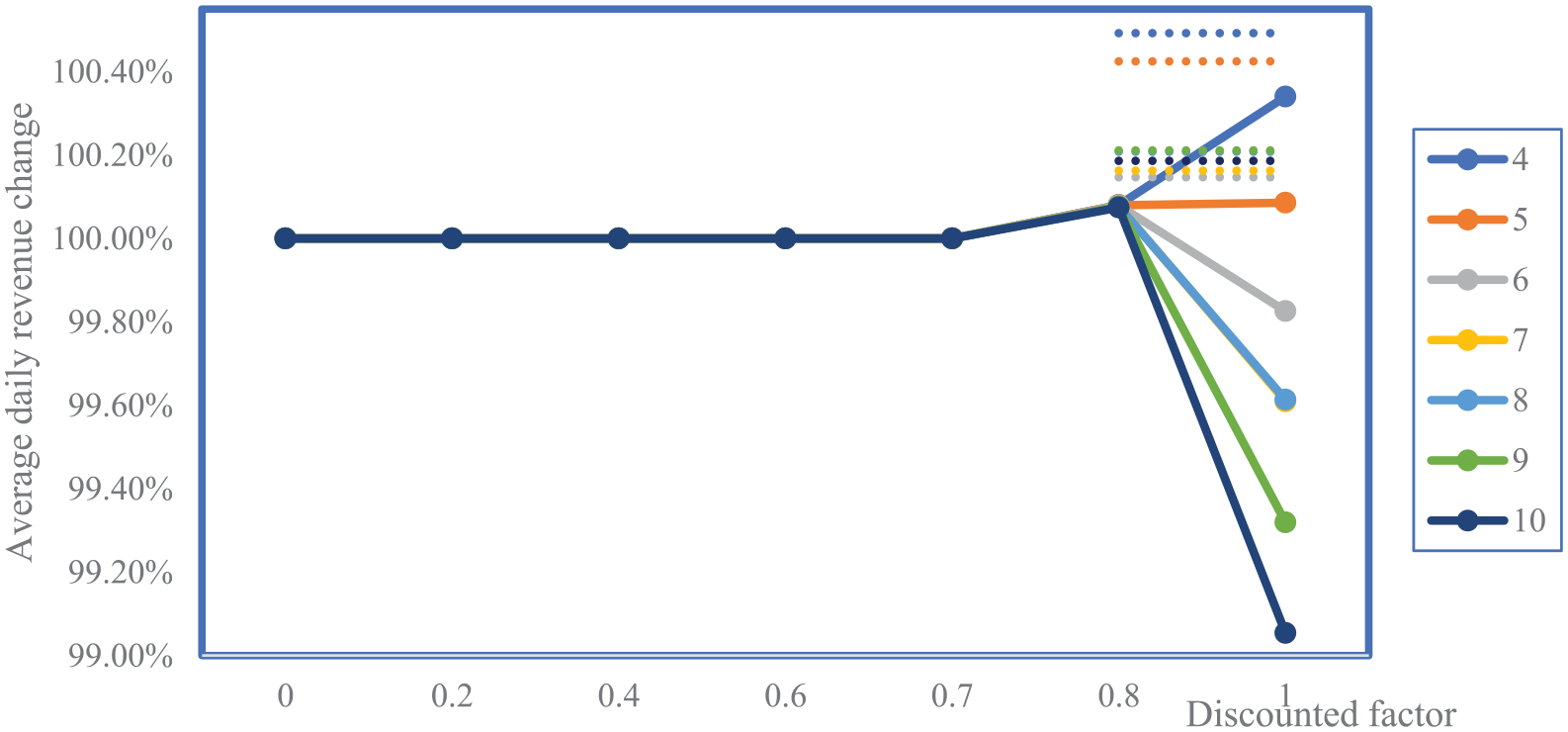
Average daily revenue changes with different transaction costs C and discounted factors $α^{D_{2}}$ ( $η = 92 %$ ).

4.3. Effect of Forecast Accuracy

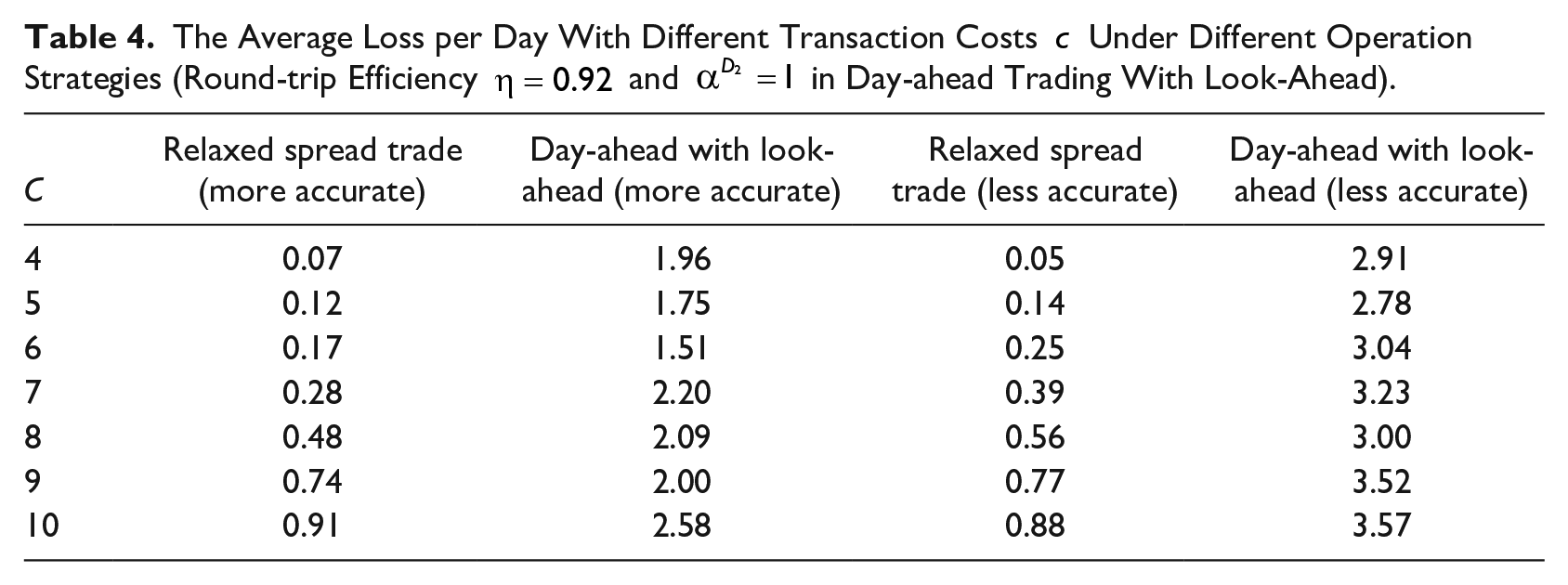
The accuracy of price forecasts may be crucial. To investigate this further we considered the effect of less accurate forecasting and the use of perfect predictor’s. Forecasting day-ahead electricity prices using only the previous prices (without the other predictor variables) gives less accurate forecasts with R²-squares of .61 and .49 for one and two days ahead respectively. The inaccuracy of the forecasts reduced the average daily revenue by £5. Table 4 reports average daily losses (the sum of losses on days with losses divided by the total number of days), and surprisingly for day ahead trading the difference in losses in day-ahead spread trading is minimal, regardless of whether the less accurate forecast information is used. But for day-ahead trades with look-ahead, there is a larger difference in losses (54.0% on average). This further demonstrates the robust advantages of day-ahead spread trading.

Table 4.

The Average Loss per Day With Different Transaction Costs $c$ Under Different Operation Strategies (Round-trip Efficiency $η = 0.92$ and $α^{D_{2}} = 1$ in Day-ahead Trading With Look-Ahead).

C	Relaxed spread trade (more accurate)	Day-ahead with look-ahead (more accurate)	Relaxed spread trade (less accurate)	Day-ahead with look-ahead (less accurate)
4	0.07	1.96	0.05	2.91
5	0.12	1.75	0.14	2.78
6	0.17	1.51	0.25	3.04
7	0.28	2.20	0.39	3.23
8	0.48	2.09	0.56	3.00
9	0.74	2.00	0.77	3.52
10	0.91	2.58	0.88	3.57

For comparability, we have chosen a twenty-four hours look-ahead time window in the continuous trading model. Table 5 shows the backtesting results. The average daily return for continuous trading is remarkably lower, being only 28 percent of that for spread trading.

Table 5.

The Revenues per Day for Continuous and Spread Trading (£).

c	η = .8		η = .92		η = .95
c	Continuous	Relaxed spread trade	Continuous	Relaxed spread trade	Continuous	Relaxed spread trade
5	16.93	61.46	20.63	72.94	21.54	75.78
6	15.67	58.98	19.25	70.05	20.09	72.84
7	14.18	56.36	18.1	67.57	18.78	70.36
8	12.78	53.77	16.39	64.94	17.17	67.68
9	11.89	51.43	14.79	62.32	15.87	65.13
10	10.79	49.42	14.1	59.84	14.36	62.57

This is due to two factors. Firstly, it is in the data and the main observation is that there are higher spreads in the day-ahead prices compared to the intraday prices (recall section 3.1). Consequently, there is greater arbitrage potential in the day-ahead market. Thus, it is not mainly due to forecasting errors. For example, assuming that the battery operator has perfect foresight, that is, that the battery schedules at the actual price, the average daily return from the day-ahead market would be £90.12, while the average daily return for continuous trading would be £70.3. But forecasting is a factor and the second observation is that greater forecasting ability seems to be required in continuous trading with look-ahead. The results in Table 5 for continuous trading are less than 30 percent of the average return per trade when the operator has perfect foresight, compared to above 60 percent for the spread trading.

The effect of the length of the look-ahead window is illustrated in Figure 3. Look ahead windows of 4, 6, 8, 12, and 24 are shown, for transaction costs of 5 and 10. When transaction costs are relatively low, the look-ahead window does not significantly affect average daily returns. There are presumably attractive short-term opportunities. However, higher transaction costs require a longer time window in order to identify the larger spreads.

Figure 3.

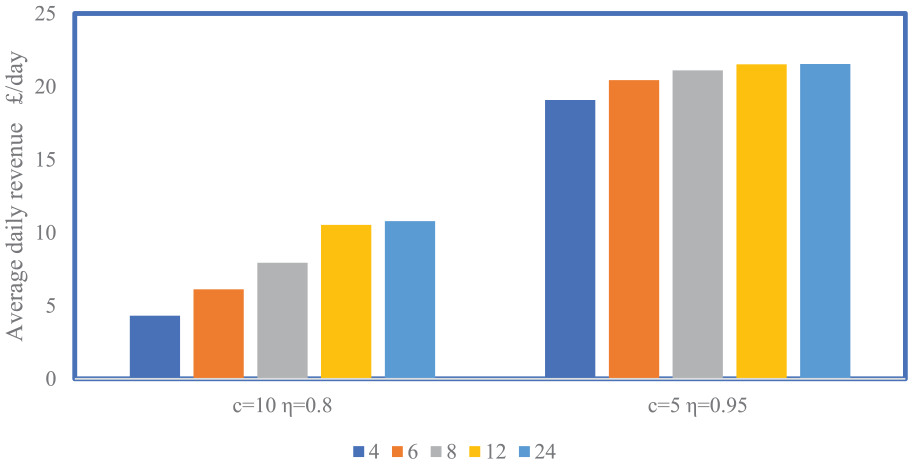
Average daily revenue with different look-ahead windows (in hours).

5. Systematic Effects Day-Ahead and Intra-Day

The indications from Figure 1 and Table 1 were that higher hourly price spreads could be achieved from the day-ahead auction than from close-to-real-time trading on the intra-day market. The effect of this was confirmed in the above trading results and it is the primary reason why the average performance was better for the day-ahead spread trading. The question which arises, as a consequence, is whether this is an idiosyncratic property of the GB market, or whether systematic factors are at play. Previous research on daily price formation has provided evidence of dynamic adaptation of supply quantities by generators according to market circumstances. In a detailed econometric analysis by Karakatsani and Bunn (2008), it was shown that whilst the reserve margin for capacity on the day had a negative effect on prices, as expected (supply surplus or scarcity lowered or increased prices, respectively), the lagged reserve margin to the previous day had a negative sign and thereby indicated opposite effects. It was suggested that generators tended to offer lower capacity if the previous day had shown lower prices through higher capacity and vice versa. In other words, relatively high day ahead prices will then become lower on the day and lower day ahead prices would become higher, through the capacity adaptations. Spreads between high and low prices would therefore be higher day-ahead than on the day due to generators adapting their capacity availability decisions. Evidently the market has to be sufficiently concentrated for this price effect to happen, but that is not unusual in power markets and relatively small amounts of capacity adjustments can often move prices. This effect was also manifest in some data on intra-day reserve margins, as forecast and released routinely to the market by the System Operator in GB (shown in Figure 4 for selected hours and days). For particular settlement periods (SP) on three separate days, the forecasts of de-rated reserve margins (excess capacity over forecast demand de-rated for technical reliabilities) are shown as a function of their lead-times.

Figure 4.

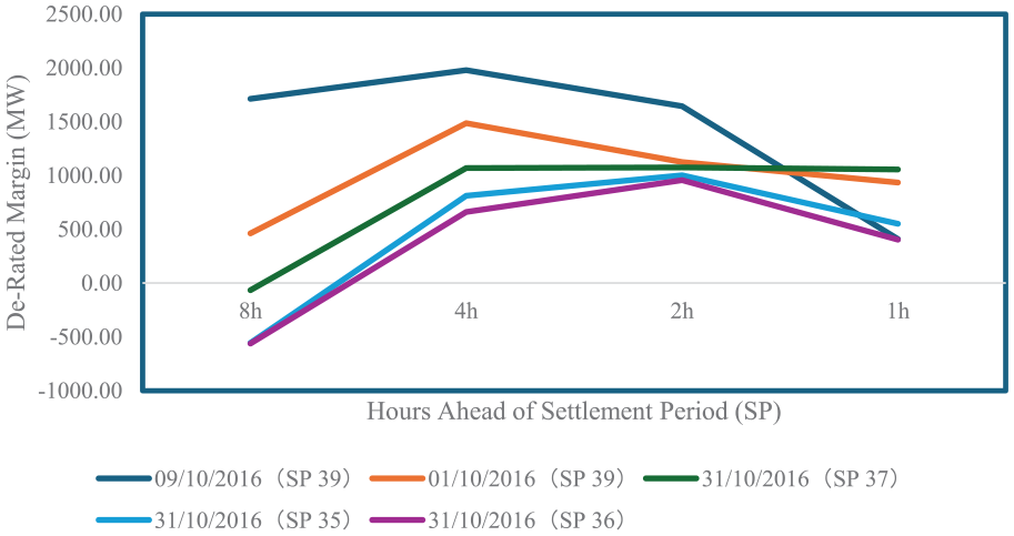
Forecast De-Rated Reserve Margins (DRM) as a function of lead times.

In this figure we see a mean reversion within the day to a DRM around 1,000 MW for real-time delivery. At eight hours ahead of delivery, when the DRM was above 1,500 MW, it moved steadily downwards, whereas when it was very low, around zero, it moved upwards. This again suggests that there would be some mean reversion in price spreads to lower values closer to real time. Notwithstanding this systematic effect, there would inevitably be other effects intraday such as demand and supply shocks to add noise and volatility, but they would be more random, whilst this systematic mean reversion in capacity adjustments is an average systematic effect of generator behavior that could generalize from this particular example. It is an example of Cournot strategies which have been widely documented in electricity markets.

6. Summary and Conclusion

Based upon backtesting with British data, the advantages of day-ahead spread trading in terms of both revenues and lower risks are demonstrated. The average daily return for continuous intra-day trading is remarkably lower on this data, than that of the day-ahead spread trading, being only 28 percent of that for spread trading. Spread trading that looks for a maximum of two trades per day can keep revenues at a higher level compared to both day-ahead with look-ahead and continuous trading with look-ahead, especially when trading costs are high. Furthermore, spread trading is effective in reducing losses per day and remains effective under sensitivity analyses for battery efficiency and transaction costs. Finally, spread trading can avoid trading losses when forecasts are less inaccurate. Evidently the comparison with continuous trading is the most remarkable and is mainly due to the nature of the data: the day ahead prices demonstrated greater spreads compared to the intraday prices, to the benefit of arbitrage traders. It is perhaps not surprising to see smaller spreads intraday as high or low prices day-ahead may prompt more or less generation supply to be made available intraday, thus closing the price spreads. Thus, we consider these results may not be idiosyncratic and they should be the basis of general insight on the systematic benefits of day-ahead spread trading. Nevertheless, further research on a variety of different markets will be worthwhile to characterize the relative benefits of different arbitrage trading approaches.

Overall, the business context for battery storage has been showing very strong growth. In GB, in 2022, there was 1.6 GW of battery storage operating in the wholesale market, whilst there was 12 GW either under construction or with full development consents, and a further 19 GW in development (National Grid 2022). Of all of this, according to Modo Energy (2024), there was 4.5 GW of batteries active in the GB wholesale market by at the beginning of 2024 (excluding domestic and EVs), representing 120 sites and 41 asset owners. Evidently there must have been persuasive investment cases for all these assets to be financed. Whilst batteries can achieve revenue streams for various flexibility and reserve services, as well as attract capacity market support, arbitrage trading appears to be a major component and benchmark for profitability (LCP 2021). We observe therefore that the daily operational profit contributions that we have identified in this comparative analysis of wholesale arbitrage trading translate into a significant component of the business cases for battery investments in GB. It is however likely that arbitrage with the balancing markets, where low volumes are compensated by higher price volatilities, will become increasingly important going forward. This would also be a promising direction for further research.

Footnotes

Appendix

Table A3.

Correlation Matrix.

	DAP	WIND	SOLAR	GAS	COAL	LOAD	DRM
DAP	1.00	−0.08	−0.07	0.73	0.63	0.18	−0.25
WIND	−0.08	1.00	−0.13	0.03	−0.01	0.15	0.56
SOLAR	−0.07	−0.13	1.00	−0.11	−0.05	0.25	−0.21
GAS	0.73	0.03	−0.11	1.00	0.85	0.07	−0.06
COAL	0.63	−0.01	−0.05	0.85	1.00	−0.01	−0.09
LOAD	0.18	0.15	0.25	0.07	−0.01	1.00	−0.52
DRM	−0.25	0.56	−0.21	−0.06	−0.09	−0.52	1.00

Acknowledgements

The authors are grateful for constructive feedback from referees.

Declaration of Conflicting Interests

The author(s) declared no potential conflicts of interest with respect to the research, authorship, and/or publication of this article.

Funding

The author(s) disclosed receipt of the following financial support for the research, authorship, and/or publication of this article: This work is supported by the National Natural Science Foundation of China under Grant No.72374018, No.72021001.

References

Abramova

Bunn

2020. “Forecasting the Intra-Day Spread Densities of Electricity Prices.” Energies 13 (3): 687.

Abramova

Bunn

2021. “Optimal Daily Trading of Battery Operations Using Arbitrage Spreads.” Energies 14 (16): 4931.

Aliasghari

Zamani-Gargari

Mohammadi-Ivatloo

2018. “Look-Ahead Risk-Constrained Scheduling of Wind Power Integrated System with Compressed Air Energy Storage (Caes) Plant.” Energy, 160: 668–77.

Arcos-Vargas

Á.

Canca

Núñez

2020. “Impact of Battery Technological Progress on Electricity Arbitrage: An Application to the Iberian Market.” Applied Energy 260: 114273.

Daggett

Qadrdan

Jenkins

2017. “Feasibility of a Battery Storage System for a Renewable Energy Park Operating with Price Arbitrage.” In 2017 IEEE PES Innovative Smart Grid Technologies Conference Europe (ISGT-Europe), Turin, Italy, 1–6. New York, NY: IEEE.

Delille

Francois

Malarange

2012. “Dynamic Frequency Control Support by Energy Storage to Reduce the Impact of Wind and Solar Generation on Isolated Power System’s Inertia.” IEEE Transactions on Sustainable Energy 3: 931–9.

Elexon. 2024. “Balancing Market Reporting Service.(BMRS)” https://bmrs.elexon.co.uk/.

Elexon. 2021. “Consultation on the Market Index Definition Statement (MIDS) Review 2021.” https://www.elexon.co.uk/consultation/consultation-on-mids-review-2021/.

Foster

2017. “Understanding the “Arbitrage” Value of a Large Battery in SA.” https://reneweconomy.com.au/understanding-the-arbitrage-value-of-a-large-battery-in-sa-16154/.

10.

Jiang

D. R.

Powell

W. B.

2015. “Optimal Hour-Ahead Bidding in the Real-Time Electricity Market with Battery Storage Using Approximate Dynamic Programming.” INFORMS Journal on Computing 27: 525–43.

11.

Jiang

D. R.

Powell

W. B.

2017. “Risk-Averse Approximate Dynamic Programming with Quantile-Based Risk Measures.” Mathematics of Operations Research 43(2): 554–79.

12.

Juárez

C. Q.

Musilek

2021. “Optimal Real-Time Scheduling of Battery Operation Using Reinforcement Learning.” In 2021 IEEE Canadian Conference on Electrical and Computer Engineering (CCECE), ON, Canada, 1–7. New York, NY: IEEE.

13.

Karakatsani

Bunn

D. W.

2008. “Intra-day and Regime-Switching Dynamics in Electricity Price Formation.” Energy Economics 30: 1776–97.

14.

LCP. 2021. “Is Battery Storage a Good Investment Opportunity?” https://www.lcp.com/energy/publications/is-battery-storage-a-good-investment-opportunity.

15.

Lucas

2019. “Throughput vs. Revenues: Making the Most From Battery Storage.” https://www.current-news.co.uk/blogs/throughput-vs-revenues-making-the-most-from-battery-storage.

16.

Marchgraber

Alács

Guo

Gawlik

Anta

Stimmer

Lenz

Froschauer

Leonhardt

2020. “Comparison of Control Strategies to Realize Synthetic Inertia in Converters.” Energies 13 (13): 3491.

17.

Modo Energy. 2024. “Benchmarking.” https://modoenergy.com/benchmarking/indices?industry=installedPower&settings=%257B%2522viewBy%2522%253A%2522growth%2522%257D.

18.

Mohsenian-Rad

2015. “Optimal Bidding, Scheduling, and Deployment of Battery Systems in California Day-Ahead Energy Market.” IEEE Transactions on Power Systems 31 (1): 442–53.

19.

National Grid. 2022. “Potential Electricity Storage Routes to 2050.” https://www.nationalgrideso.com/document/273166/download#:~:text=Today’s%20GB%20electricity%20storage%20technology,capacity%2C%20a%20much%20higher%20ratio.

20.

Núñez

Canca

Arcos-Vargas

Á.

2022. “An Assessment of European Electricity Arbitrage Using Storage Systems.” Energy 242: 122916.

21.

Salles

Aziz

M. J.

Hogan

W. W.

2016. “Potential Arbitrage Revenue of Energy Storage Systems in PJM During 2014.” In 2016 IEEE Power and Energy Society General Meeting (PESGM), Boston, MA, 1–5. New York, NY: IEEE.

22.

Shu

Jirutitijaroen

2013. “Optimal Operation Strategy of Energy Storage System for Grid-Connected Wind Power Plants.” IEEE Transactions on Sustainable Energy 5 (1): 190–99.

23.

Staffell

Rustomji

2016. “Maximising the Value of Electricity Storage.” Journal of Energy Storage 8: 212–225.

24.

Wang

Y. S.

Dvorkin

Fernandez-Blanco

B. L.

Qiu

Kirschen

D. S.

2017. “Look-Ahead Bidding Strategy for Energy Storage.” IEEE Transactions on Sustainable Energy 8: 1106–1117.

25.

Sioshansi

Marano

2014. “A Stochastic Dynamic Programming Model for Co-optimization of Distributed Energy Storage.” Energy Systems 5 (3): 475–505.

Daily Episodic and Continuous Arbitrage Trading With Electric Batteries

Abstract

Keywords

1. Introduction

2. Formulations

2.1. Day-Ahead Trading With and Without Look-Ahead

2.2. Continuous Trading With Look-Ahead

3. Data and Forecasts

3.1. Forecasting the DAP

3.2. Forecasting the MIP

3.3. Other Details

4. Results

4.1. Day-Ahead Spread Trading

4.2. Day-Ahead Trading With Look-Ahead

4.3. Effect of Forecast Accuracy

5. Systematic Effects Day-Ahead and Intra-Day

6. Summary and Conclusion

Footnotes

Appendix

Acknowledgements

Declaration of Conflicting Interests

Funding

References