Sage Journals: Discover world-class research

Abstract

Aggregators are increasingly using portfolios of various end-user resources such as local renewable generation, batteries, EVs, and demand-side management to participate in the electricity markets as virtual power plants. Whilst the smart control of energy within buildings is well established for cost optimization, the prospect of an aggregator collaborating with the energy managers of buildings to trade electricity in the wholesale markets is under researched. This paper uses a state-of-the-art architectural simulator to model the thermal inertia of a typical high-rise building in London and represent the thermodynamics of its hourly occupancy and weather responses. The building is simulated as a virtual battery by manipulating the HVAC settings. Price arbitrage on the electricity wholesale market and contracting with the local distribution network for flexible reserve services are both feasible and profitable. It is concluded that aggregators can apparently use buildings as additional assets within their trading portfolios.

JEL Classification: L85 and L94.

Keywords

electricity storage buildings trading aggregators

1. Introduction

Whilst the energy management of a commercial building has historically been a passive process relying upon the installation of energy efficient appliances and insulation, there are now more opportunities for the optimization of buildings as active energy resources within the electricity markets. These opportunities emerge from a combination of smart technologies and the more liberalized market arrangements for end-user participation. Intelligent systems for the consumption of electricity are becoming widely adopted as advanced location sensors and software can control a building’s responses to hourly variations in electricity prices, whilst the use of weather forecasts in predictive algorithms means that the heating and air-conditioning services can have look-ahead functions in their control settings. In addition, buildings may have roof-top solar generation, heat pumps and batteries, as well as conventional back-up generators, so that they can manage their resources to meet fluctuating needs and export power to the grid whenever the opportunities arise. The ability of a building to buy and sell electricity is facilitated by the retail arrangements with some of the more innovative utilities and the so-called aggregators, or “virtual power plants,” who bundle the resources of end-users so that they have the sufficient scale to participate in the wholesale power markets. Policy-makers have indeed become keen to support the emergence of these new aggregators and the increased consumer engagement in power markets, not least because they can increase the energy security of the power system as a whole (EU 2017; FERC 2020).

Buildings have substantial thermal inertia in their structure such that their energy managers can delay or advance consumption (e.g., for heating, refrigeration, and air conditioning) without degrading the ambient quality to the occupants. Whilst smart controls of buildings have been well established for cost optimization and demand response to time-of-use prices has been extensively researched (e.g., Vesterberg et al. 2016), it is an open research topic if buildings can be profitable as an additional storage technology which aggregators can include in their portfolios of trading resources. Careful forecasting and scheduling of the heating and cooling controls are crucial elements that aggregators need to model if they are to make effective use of buildings as tradeable assets. In particular, modeling the thermal inertia of the building, in terms of its fabric and use, needs to be linked to tradeable volumes and power prices to anticipate revenues. We observe that the economic value of trading the thermal inertia of a building in the wholesale market for power and the flexibility markets for reserve power capacity has not been fully researched. That is the motivation of this research. A key consideration is whether the power system operators can reliably contract with buildings (indirectly though aggregators) to provide alternative battery-like storage services.

Energy storage has become particularly valuable with the rapid penetration of renewable power, as periods of power surplus and scarcity become more extreme and need to be managed. The economics of buildings as storage are potentially favorable. The building and its facilities are constructed for other purposes and so, unlike investment in dedicated batteries, the profits from trading opportunities do not have to contribute to any capital costs, except for the relatively low cost of installing a suitable control system. This research therefore seeks to apply that conjecture and develop a proof of concept that a building can be operated in a manner that allows it to capture additional revenues from trading in the power market as a battery.

The research question is addressed by means of a state-of-the art architectural simulator applied to a typical building located in the center of London. An aggregator uses the building to trade within the British wholesale electricity market and also to offer reserve services to the local grid operator. Following a review of related background research in the next section, Section 3 explains the formulation and behavior of the building model, as well as introducing the markets in which it could operate. Section 4 presents the selected market scenarios and Section 5 discusses the calibrated case studies. Section 6 concludes the study.

2. Background Research

Energy consumption in the built environment is an extensively researched field. A wide range of analytical methodologies have been created and investigated in order to understand how weather factors interact with electricity demand in various building types and their configurations (Amasyali and El-Gohary 2018). There are computationally-intensive physical models of the buildings that process vast amounts of data via machine learning algorithms and statistical processes to predict and control the load profiles of the buildings (Godina et al. 2018; Huang et al. 2014; Runge and Zmeureanu 2019). The techniques of Support Vector Machines and Artificial Neural Networks have exhibited superior accuracy in this respect over conventional statistical methods (Farzana et al. 2014; Ferlito et al. 2015; Massana and Colomer 2016; Mat Daut et al. 2017; Paudel et al. 2015). The physical modeling often uses the thermodynamic properties of the buildings, but their representations tend to be deterministic rather than stochastic. Some use resistor-capacitance (RC) analogies between the electrical resistance and capacitance of a circuit to the thermal counterparts of a building. Commercial software such as EnergyPlus, eQuest, and Ecotrect are widely used in practice. They are computationally intensive but facilitate a high degree of accuracy. For more rapid computations, a reduced-order regression model, estimated for example from EnergyPlus simulations, can be applied for prediction and control, as in Cole et al. (2014). Optimizations that consider the potential scope beyond the individual buildings to local microgrids, distribution networks and smart cities include Jin et al. (2017), Meng et al. (2019), and Joe et al. (2020). However, all of this intelligent management of buildings is directed toward efficient operations and does not explicitly consider the potential asset value to aggregators from trading them in the wholesale power markets as battery-like assets.

Electricity storage in general has moved from being a fringe resource in the form of pumped-hydro to a crucial element in the energy transition alongside renewable generation, where batteries and perhaps hydrogen storage are necessary to accommodate the intermittency of production (Eunomia 2016; Frate et al. 2021; IRENA 2019; Ofgem 2021; Pereira da Silva and Paulo 2019). Further, the effect of renewables’ increasing price volatility (Rintamäki et al. 2017) makes the price arbitrage profits from storage more attractive. Even in the residential segment, end-consumers can complement their domestic roof-top solar with batteries to minimize their electricity costs through load shifting and price arbitrage (McKenna et al. 2013). The potential for battery resources to trade arbitrage opportunities in the wholesale market is attractive in terms of operating profit contributions (Abramova and Bunn 2019; Giuletti et al. 2018), but it is yet to be proven whether such revenues are sufficient to justify battery investments (Arcos-Vargas et al. 2020; Metz and Saraiva 2018), despite the steady reductions in battery capital costs (Lazard 2021).

Apart from the capital costs of batteries, there are losses due to the process of charging and discharging, measured through round-trip efficiency (RTE). Makibar Puente and Navarte Fernández (2015) report an RTE for a typical Li-ion battery system to be close to 85 percent. Discrepancies with RTEs reported by battery manufacturers, for example, 90 percent for the Tesla Powerwall (Tesla 2020), and a fully installed energy storage system (ESS), may be due to the losses in the inverter, connections, and other elements of the ESS. RTE losses must be accounted for when considering arbitrage trades, and consequently the buy-sell price spreads must be large enough to offset not only these RTE losses but also any trading transaction costs and use of system charges. Furthermore, electrochemical batteries degrade over time. Bishop et al. (2016) conclude that when batteries provide active short-term reserve services to the electricity system operator their lives are shortened by about 15 percent. Nevertheless, Arcos-Vargas et al. (2020) predicted that the capital investment of Li-ion batteries to perform wholesale price arbitrage would break even if trends in RTE, capital costs, and battery degradation continued improving at their historical rate.

Unlike Li-ion, pumped hydro or power-to-gas technologies, buildings offer a further alternative storage solution through power-to-heat using their thermal mass. The make-up of this thermal mass encompasses the building structure and envelope, internal elements (fittings, furnishing, etc.), and the air volume (Reilly and Kinnane 2017). It helps stabilize internal temperatures by absorbing or releasing thermal energy, depending on temperature differentials with its surrounding environment. The lags involved in this temperature adjustment process by the thermal mass, together with the heating, ventilation, and air-conditioning system (HVAC), provide the basis for dynamic management of its energy consumption and its potential to act as flexible storage. Le Dréau and Heiselber (2016) provide a bibliometric review of the technical aspects of flexibility in the energy consumption of buildings, but do not cover links to trading this flexibility in the market. Similarly, Raman and Barooah (2020) show that energy storage in a building using a variable-air-ventilation HVAC system can reach an RTE close to one, but do not extend the analysis to consider its market trading implications. Furthermore, since the electrical energy is stored in the thermal mass, the degradation of storage capacity through repeated storage cycles can be assumed to be negligible.¹ And there is negligible capital cost attributable to the process as the building’s structure, fittings, furnishing, and air volume are present regardless of whether they are used for energy storage. Thus, despite the apparent awkwardness of operating a building as a battery, there are in principle some attractive performance characteristics. Furthermore, this awkwardness can be mitigated by using AI-enabled algorithms, as already in use by aggregators to optimize the scheduling of their portfolios of distributed energy resources. The research contribution of this paper is therefore to analyze whether these technical advantages can be monetized through market trading. We are not aware of a detailed analysis elsewhere of the financial returns to operating buildings as battery assets within an aggregator’s trading portfolio.

3. Modeling the Thermal Mass of Buildings

The OpenStudio modeling platform was selected for its high-degree of programmability and widespread use as the state of the art by designers of the built environment. Developed by the National Renewable Energy Laboratory in collaboration with the US Department of Energy, OpenStudio is an opensource building performance tool (OpenStudio 2022). It is composed of several components to represent the physical properties of a building. Most importantly the whole-building energy consumption is estimated using EnergyPlus. We were reassured from the 96 percent accuracy previously reported for Energy Plus (Dudley et al. 2010). The built-in FloorspaceJS programme facilitates two-dimensional building design. The designed spaces take a parallelogrammatic form on each floor of the building. Floors are then stacked in the preferred order to form a multi-story structure. The user is also able to assign materials of varying thermal performances to the partitions created on FloorspaceJS. The building’s material specification will dictate its thermal mass.

To simulate the impact of the weather on the energy consumption of the building, we used the Test Reference Year (TRY) weather database created by The Chartered Institution of Building Services Engineers, being the average of thirty years of weather data from the UK Meteorological Office for specific locations (CIBSE 2016). The dataset contains a range of hourly meteorological variables (e.g., dry and wet bulb temperature, precipitation, wind direction and speed, solar irradiance, and cloud coverage) over a 8,760-hour period (i.e., one year). The selected dataset, representing the typical weather in London over a year, is fed into the building model. It imposes a thermodynamic load on the building, which, when necessary, must be counteracted by the HVAC system to ensure safe and comfortable internal conditions for the users. For a domestic specification, the thermal loads associated with regular living behaviors (“schedules” in the model) are also estimated, and involve the regular use of lighting, home appliances, and IT. “Priority” schedules are included to over-ride regular schedules in order to account for special days, such as holidays and weekends.

3.1. The Test Model in Detail

Our Open Studio Building (the “OSB”) designed as the experimental test for the proof-of-concept simulation is fifteen floors tall, with the ground floor allocated to office space, and the remaining fourteen floors to dwellings. Each residential floor has eight apartments, with the following dimensions: 8 m × 11.5 m × 3.05 m. The concrete building is located in London, with the entrance being east-facing. A glazing ratio of 0.3 has been selected in accordance with the range of 0.3 to 0.45, suggested in Goia (2016). Glazing ratio is proportional to solar gains. By selecting the lower-bound ratio, less heat is provided to the building throughout the year. This results in an optimistic case in Winter months, as there is more energy capacity to trade, and a conservative case in Summer months. Adjacent buildings will cast shadows and are assumed to have the same dimensions as the OSB. A lateral separation of 20 m between buildings has been selected, following historical guidance by the UK Department for Communities Local Government (GLA 2016). Even though the selected height of the shading array may be an over-conservative estimate, in practice it is unlikely that a typical high-rise building would not be subject to any shading.

Schedules have been included to accurately replicate the heat gains that would arise from regular occupancy. For the offices, an 8:00 to 17:00 occupancy schedule has been set from Monday to Friday, while a null occupancy schedule has been set for weekends. The opposite occupancy schedule has been implemented for the dwellings, in which most occupants leave between 7:30 and 8:30, some come back temporarily for lunch, and finally occupants gradually return from 16:00 to 21:30. More constant occupancy schedules are programmed for the weekends, with a minimum occupancy of 70 percent on Sundays and 65 percent on Saturdays. The occupancy per residential floor has been set at twenty-six people, 3.25 per apartment as per the English Housing Survey Floor Space (MHCLG 2017), while the capacity per office has been set at twelve people as per the UK Employment Density Guide Ed. 3 (HCA 2015). Spaces have been equipped with electrical equipment in order to simulate day-to-day loads, such as cooking, home appliances, IT, and lights, in the offices and apartments. Thermal radiance factors for each piece of equipment have been derived from the ***ASHRAE² Fundamentals Handbook (ASHRAE 2001). The utilization profile for these loads resembles the occupation profile, with morning and afternoon peaks during weekdays and constant profiles on weekends. It is worth noting that these schedules are stylized assumptions. Considering the growing post-pandemic trend of working from home, it is likely that a larger residential occupancy rate may be observed during weekdays. The assumed schedules do however provide a conservative case, as the increased power use resulting from the higher volume of residents would actually increase the building’s potential “battery” capacity (discussed below).

Thermal mass has been introduced into the model via nominal structural components, such as floor slabs (175 mm concrete), exterior walls (300 mm concrete), and interior partitions (100 mm concrete), with internal insulation. However, the structural designs of load-bearing elements, such as beams and columns, has not been modeled. Their absence will result in an underestimate of the building’s true thermal mass. The decision to use internal insulation is founded on its 20 percent efficiency boost vis-à-vis its external counterpart (Reilly and Kinnane 2017). Additional thermal storage has been introduced in the form of furnishing. According to Johra et al. (2019), internal furnishing can increase a building’s time constant (i.e., the ability to store and retain heat energy) by up to 42 percent. The HVAC system is composed of an air-to-air heat pump with a Coefficient of Performance (COP) of 2.5, based on the minimum COP requirement stated in the British building standards (BSI British Standard 2022). A heat pump system was selected based on the increasing trend in the United Kingdom of equipping new buildings with sustainable energy sources. The multi-storey building was better suited to an air-to-air system, compared to its ground-source counterpart. Heat pumps commonly have higher COPs, which would result in a lower potential capacity to be traded in the market. Humidifiers were installed to maintain internal relative humidity between 30 percent and 60 percent, as per ASHRAE’s recommendations (ASHRAE 2016).

For the building to operate like a battery, internal temperatures must be allowed to fluctuate within a range that does not discomfort building users. The HVAC’s operating range of 19°C to 24°C has been derived from ASHRAE 55-2010 thermal comfort guidelines. Figure 1 shows how the comfort operative temperature ranges according to outdoor temperature. Prevailing Mean Outdoor Air Temperatures (PMOAT) have been calculated for each month on a weekly basis. In winter months, PMOATs did not exceed 10°C, therefore according to the graph, the minimum allowable temperature is 18.5°C (with a 90% occupant acceptance). A thermal comfort band from 19°C to 23.5°C was therefore selected for winter. In summer months, PMOATs oscillate between 12°C and 14°C. Hence, an upper bound set-point of 24°C and a lower bound set-point of 20°C have been selected. This methodology assumes that less than 10 percent of occupants (thirty-six residents and ten employees) will feel uncomfortable with these temperature bounds.

Figure 1.

Acceptable operative temperature ranges (ASHRAE 2010).

Understanding the HVAC load profile is crucial to determining the OSB’s ability to operate as a battery in the electricity market. The thirty-year average weather variables using the London TRY database provide a base case from which different sensitivity elements are assessed.

The sensitivity analysis of the building’s energy consumptions was done by observing the impact of removing various design elements individually from the base model. Table 1 shows the seven sensitivities evaluated on an hourly basis for the 8,760 hours in the test year.

Table 1.

Impact of Model Configuration on the OSB’s HVAC Consumption.

Impacts on HVAC	No. shade	No. kitchen	No. lights	No. people	No. heat loads^a	Nothing^b	No. thermal mass^c
Total annual change (%)	−1.11	−1.56	−5.03	0.34	−28.48	−29.38	−28.51
Mean hourly change (%)	−6.36	5.49	−4.50	−0.51	−65.43	−69.80	−181.67
Hourly mean absolute difference (kWh)	2.14	3.28	4.46	0.69	20.72	18.62	14.50

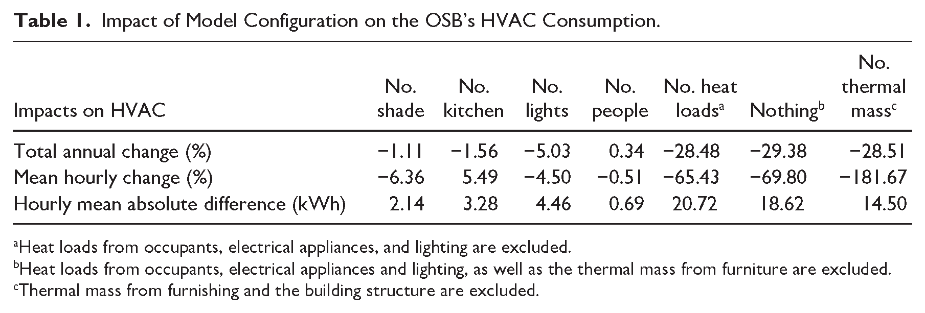
Heat loads from occupants, electrical appliances, and lighting are excluded.

Heat loads from occupants, electrical appliances and lighting, as well as the thermal mass from furniture are excluded.

Thermal mass from furnishing and the building structure are excluded.

Total Annual Change (TAC): Captures the overall change in HVAC consumption between the base case and a sensitivity case.

T A C = \frac{\sum_{h = 1}^{8760} (Q_{b, h} - Q_{a, h})}{\sum_{h = 1}^{8760} (Q_{b, h})}

Mean Hourly Change ( $μ_{Δ}$ ): Considers potential seasonal effects on consumption deviations.

μ_{Δ} = \frac{\sum_{h = 1}^{8760} (\frac{Q_{b, h} - Q_{a, h}}{Q_{b, h}})}{8760}

Hourly Mean Absolute Difference (HMAD): Captures the overall magnitude of the hourly changes in consumption.

H M A D = \frac{\sum_{h = 1}^{8760} | Q_{b, h} - Q_{a, h} |}{8760}

Where $Q_{b, h}$ is the hourly HVAC load (kWh) from the base case and $Q_{a, h}$ is the hourly HVAC load (kWh) from the sensitivity case.

Thus, in Table 1 we see that the thermal mass decreases total yearly HVAC consumption by 28.51 percent, thereby emphasizing its importance. The average monthly representation of this hourly behavior can be observed in Figure 2. HVAC consumption in the “No Thermal Mass” sensitivity fluctuates more than in the base case. In cooler months, HVAC loads are greater at night than in the “No Thermal Mass” case. This is because the HVAC system must make up for the thermal energy that has not been amassed throughout the day. Similarly, in warmer months, HVAC loads are greater during the day, as the building has not been cooled during the night and so the HVAC system must consume more energy to cool the OSB during the day.

Figure 2.

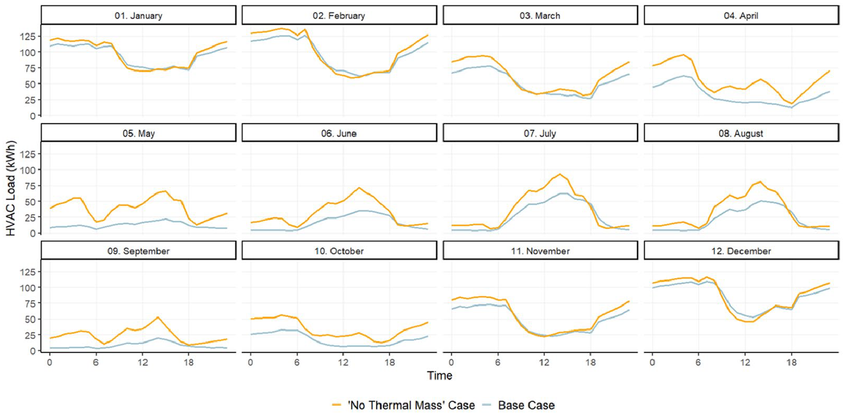
Effect of thermal mass on the OSB’s average HVAC load profile by month.

The shading array decreases total annual HVAC consumption by 1.11 percent (Table 1), with a minimum of −22.41 percent in September and a maximum of 8.55 percent in April. The cooling effects provided by shading on the building are displayed in Figure 3. In summer months, the shade cools the building, thereby alleviating the cooling load between sunrise and sunset. Given that London’s latitude imposes a heating-dominated climate, the effects of shading are minimal in winter months, shown by the subtle difference in consumption between the two cases during this period.

Figure 3.

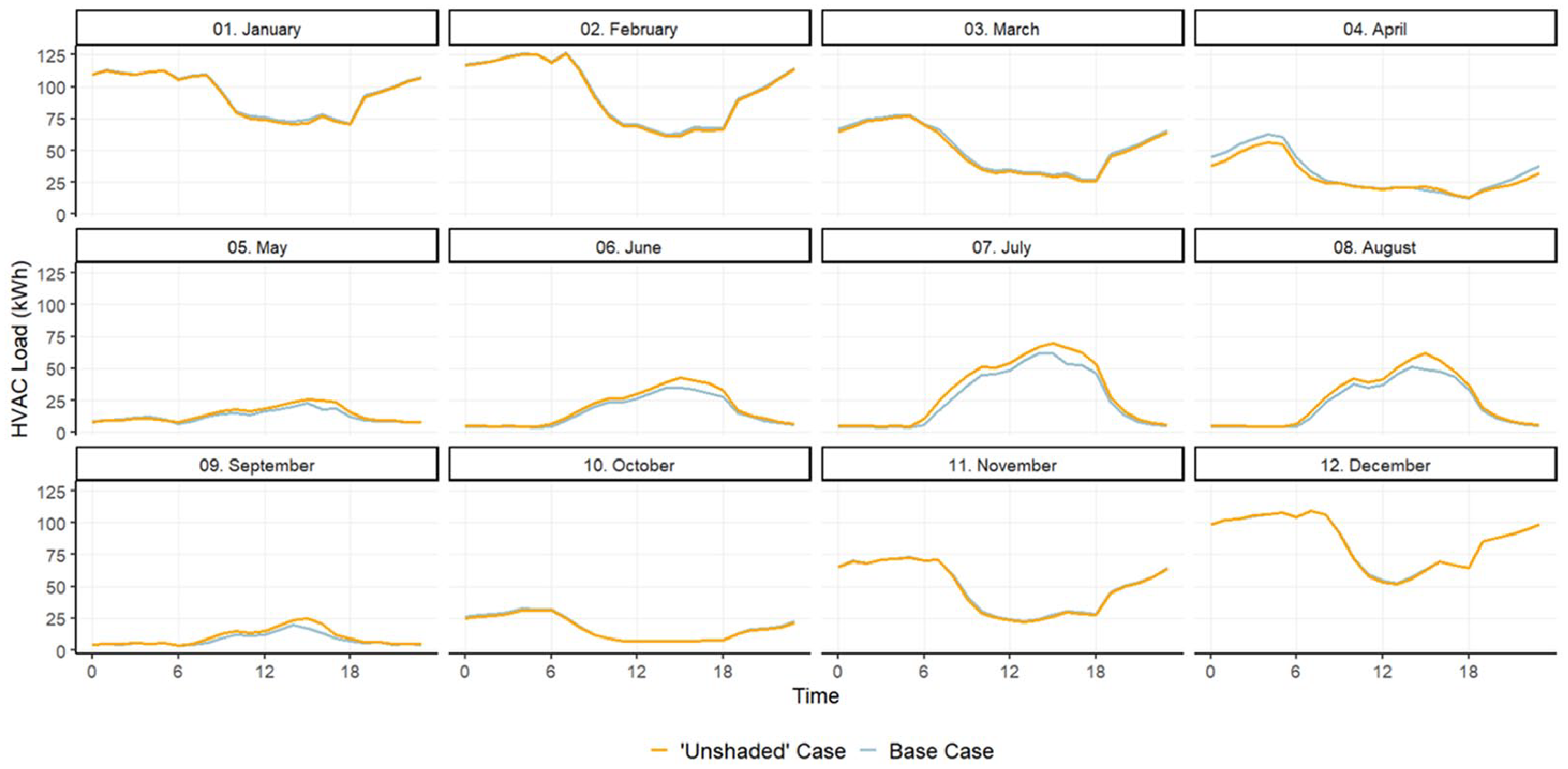
Effect of shading on the OSB’s average HVAC load profile by month.

The opposite effect can be seen when considering electrical equipment, whose operation heats internal spaces. Considering that occupants’ heat dissipation has a negligible impact on the HVAC demand, the 28.48 percent difference between the base case and one without heat loads can be mainly attributed to electrical equipment. Most electrical equipment has been programmed to follow a steady schedule, thereby heating the OSB at a relatively sustained rate. A particularly interesting case is that of kitchen appliances, as it is a more energy intensive process with significant heat losses. It has also been scheduled at discrete times, making its effects on the HVAC load more noticeable. This can be observed by the evening kinks on the base case plots in Figure 4. These kinks show an alleviation of the HVAC load in winter dominated months, yet an aggravation of cooling loads in summer months. Additionally, while the overall HVAC load due to cooking is lower, the average hourly percentage change is lower (Table 1).

Figure 4.

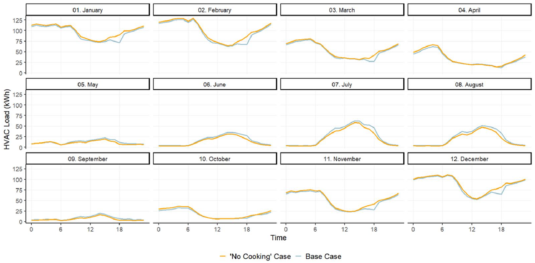
Effect of kitchen appliances on the OSB’s average HVAC load profile by month.

Market Trading Opportunities

Our working conjecture is that a building can operate as a battery by preconditioning interior spaces when an upcoming market opportunity is forecast in order to have headroom to adjust energy consumption or production. Energy is to be traded during the market opportunity to generate a profit. By “charging” and “discharging” at optimal times, these opportunistic profits can be maximized. The “charging” of the thermal mass is seen as a net import of electricity from the grid. Preconditioning internal spaces will offset the subsequent energy consumption that would have been consumed had the preconditioning not taken place. This demand reduction opportunity is equivalent to a net export into the grid, replicating the “discharging” effect of a real battery.

The market opportunity can be specified more precisely into two phases: (i) the (pre or post) conditioning period, and (ii) the service period. The service period is the time over which the OSB is being remunerated for its change in demand. The preconditioning period is the time before the service period over which the OSB will build up capacity for the service period. Not all market opportunities will have a preconditioning period, as the OSB may already have the spare capacity required for the service period. It is possible there may also be a post-conditioning period to adjust the building back to normal after the service. For a market opportunity to be profitable the revenue from the service period must outweigh the costs incurred during the pre and post conditioning periods. Given that the HVAC system controls the “charging” and “discharging” of thermal mass, its demand profile dictates the degree to which the OSB can participate in these market opportunities. Over the year, Figure 5, the OSB’s HVAC hourly consumption ranges between 251.25 and 2.15 kWh, meaning that, even though additional energy may be being consumed by, for example electrical appliances, the OSB can only “discharge" the base HVAC load normally available at that time to the electricity market. The electricity grid system operator will only recognize load reductions as negative demand (i.e., incremental supply) to the extent that they are measured against the normal baseline consumption for the service period. Demand-side management programmes have developed standard procedures for settlement in this respect (Elexon 2022).

Figure 5.

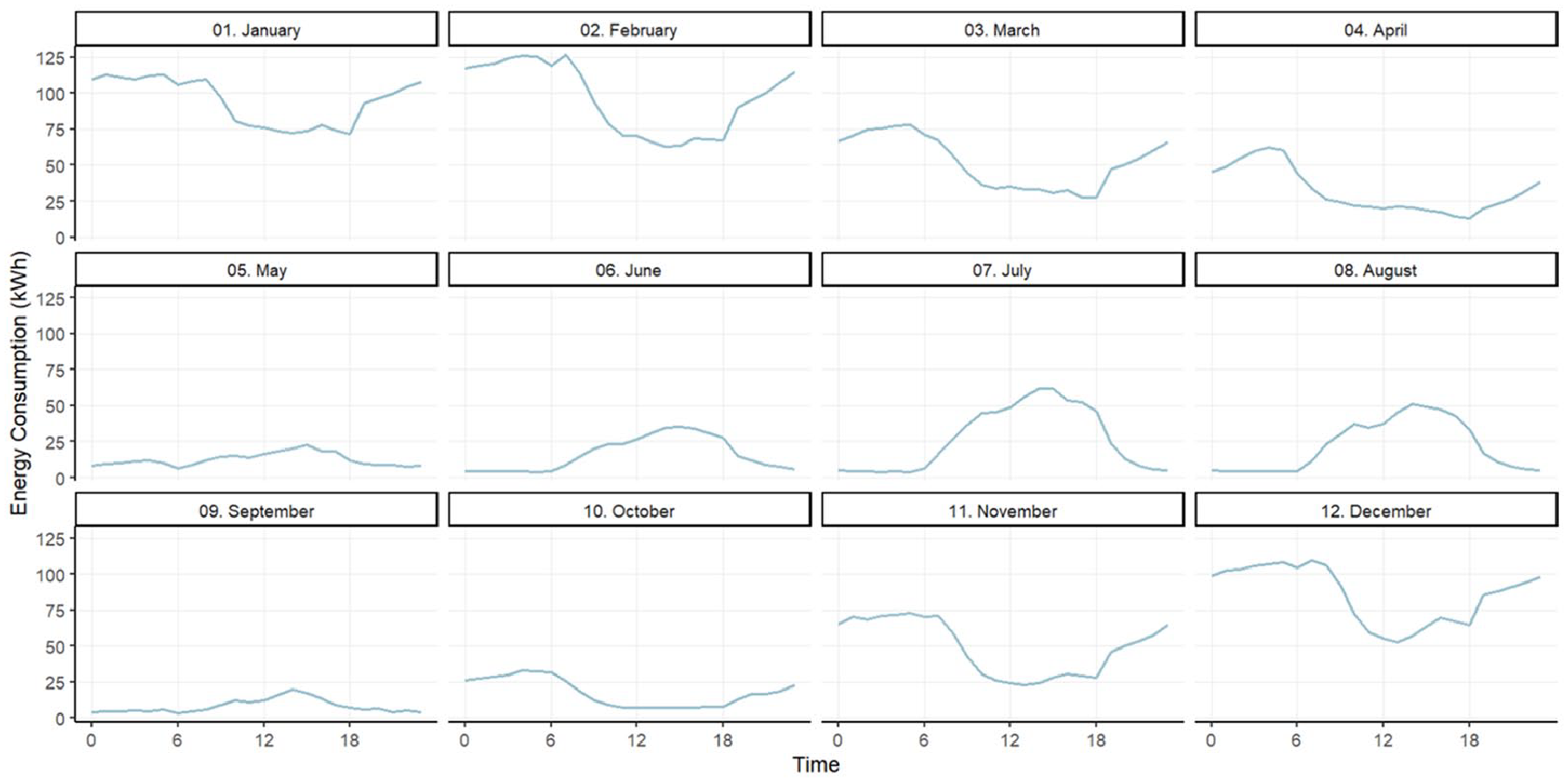
OSB’s (base case) average HVAC load profile by month.

Table 2 indicates that the most significant storage opportunities are available between November and March, as the HVAC system is employed close to 100 percent of the time.

Table 2.

Proportion of Time During Which the OSB’s HVAC System Is Operational.

HVAC Operational %	Jan	Feb	Mar	Apr	May	Jun	Jul	Aug	Sep	Oct	Nov	Dec
Heating (%)	97	96	89	52	5	0	0	0	1	40	89	98
Cooling (%)	0	0	0	0	10	27	59	49	13	0	0	0

Most wholesale electricity markets are only accessible to parties with a trading capacity in the MWh range. However, the emergence of aggregators has facilitated the incorporation of consumer-scale, distributed energy resources such as these into the energy market (Burger et al. 2016). For the purposes of this study, therefore, it has been assumed that the OSB is being aggregated with other resources to access the market utilization of its flexible energy resources at any point in time. The variables used to evaluate revenue opportunities were:

Profit contribution ( $P)$ , that is, cost reduction, is given by the revenue over the service period ( $R_{ω}$ ) minus the costs of the conditioning period ( $C_{σ}$ ):

P = R_{ω} - C_{σ}

Price differential ( $Δ λ$ ) is the ratio of the average price during the service period ( $λ_{σ}$ ) to the price during the conditioning period ( $λ_{ω}$ ):

Δ λ = \frac{(\frac{\sum_{σ = 1}^{i} λ_{σ}}{i}) - λ_{ω}}{λ_{ω}}

Average potential capacity (µQ is the hourly base HVAC consumption ( $Q_{σ}$ ) that can be offset during the service period of length ( $n$ ):

μ_{Q} = \frac{\sum_{σ = 1}^{n} Q_{σ}}{n}

To calibrate the ideal thermostat set-points for dynamic operation, the duration of the charging phase was varied and the resulting discharging length and magnitude was observed. The initial hypothesis was that a storage strategy would depend on the average potential capacity over the service period, and the season (summer and winter). Two categories of average potential capacity were selected high (80 kWh) and low (20 kWh). Therefore, four test examples were selected. The OSB was precooled in summer months and preheated in winter months. For each case, the charging period was varied in hourly increments from one to four hours. The thermostat set-point was varied in 1°C intervals between the comfort ranges shown in Figure 1, that is, decreasing it from 19°C to 23.5°C (0.5°C increment for the last test) to simulate winter months and increasing it from 24°C to 20°C to simulate summer months. It was found that a charging period of more than an hour was detrimental, because the resulting service period remained the same and HVAC consumption increased significantly. One hour of charging was found to offset the following three hours of HVAC consumption. Following a search analysis, the most effective settings were identified. In winter months, the lower bound comfort temperature was set at 19°C and in summer months the upper bound comfort temperature was set at 24°C. A discharge strategy, in which the thermostat set-points were temporarily pushed to the ASHRAE recommended limits, was implemented. The resulting optimal storage strategy for winter involved a one-hour procurement period, where the set-point was increased to 23.5°C, then decreased to 18.5°C for the three-hour service period before returning to 19°C. For summer, the set-point was lowered to 20°C for the procurement period, then, increased to 24.5°C for the three-hour service period, before returning to 24°C. With these settings established, the market trading opportunities were then evaluated. We considered arbitrage trading on the wholesale power exchange and participation of the regular tenders for reserve services to the system operator.

The study assumes that all residents of the building consent to outsourcing the HVAC regulation to the energy aggregator. We assume that the aggregator would return some portion of the profits to the residents, or to the managing agents for the building, but we do not speculate on this apportionment. The costs of installing and managing smart home hardware and software are small (in 2023, for example Hive Home^® had an installation cost of under £300 and a £4 monthly fee for the average property). We do not consider these capital and operational costs to be significant in the context of the aggregator’s business model.

4. Arbitrage Trading Proof of Concept

In the wholesale market, electricity can either be procured via forward contracts or spot purchases. Forwards are used for hedging up to three years ahead, but the most liquid product is the day-ahead auction; spot products are real-time balancing activities by the system operator to match demand and supply instantaneously. As indicated previously, the predictability of short-term weather conditions and market prices at the day-ahead stage is expected to yield a more efficient use of the thermal mass of a building. Day-ahead hourly prices from the N2EX auctions³ in GB between 1 November 2018 and 31 October 2021 were used in this study.

Simulations based upon the day-ahead prices were investigated to determine whether opportunistic operation of the OSB as a battery is financially feasible. To do so, price spreads were calculated between one hour and the following three (to cover the potential preconditioning and service periods). For the days with notable price differentials and storage capacity, HVAC control profiles were produced by incorporating the storage strategy into the HVAC schedule at the arbitrage period. The profit from the arbitrage opportunity, $P_{α}$ , is:

P_{α} = R_{ω} - C_{σ}

P_{α} = \sum (λ_{ω, d}^{D A} \times V_{ω, d}) - λ_{σ, c}^{D A} \times V_{σ, c}

Where: $λ_{ω, d}^{D A}$ is the day-ahead price at time $d$ during the service period $ω$

$V_{ω, d}$ is the volume traded at time $d$ during the service period $ω$

$λ_{σ, c}^{D A}$ is the day-ahead price at time $c$ during the procurement period $σ$

$V_{σ, c}$ is the volume traded at time c during the procurement period $σ$ .

In order to estimate the cost savings from using the building’s thermal mass as a medium to temporarily store energy, it must create a base-case of the electricity the OSB would consume if no action were taken. The aggregator can also determine the potential storage capacity by using the HVAC system as a battery, as indicated above, and whether an arbitrage opportunity is present.

If an arbitrage opportunity is identified, following the temperature bands indicated in Figure 1, in the winter storage strategy, the thermostat set-point is increased to 23.5°C during the hour before the price peak, and then dropped to 18.5°C for three hours before returning the 19°C default set-point. In the summer storage strategy, the thermostat set-point is lowered to 20°C during the hour before the price peak, and then raised to 24.5°C for three hours before returning the 24°C default set-point. Finally, the aggregator submits a bid to buy power (“charging”) and offers to sell the demand reductions (“discharging”) according to the resulting HVAC profile from the storage strategy. The cost savings are a result of comparing the cost of the base case to the control case.

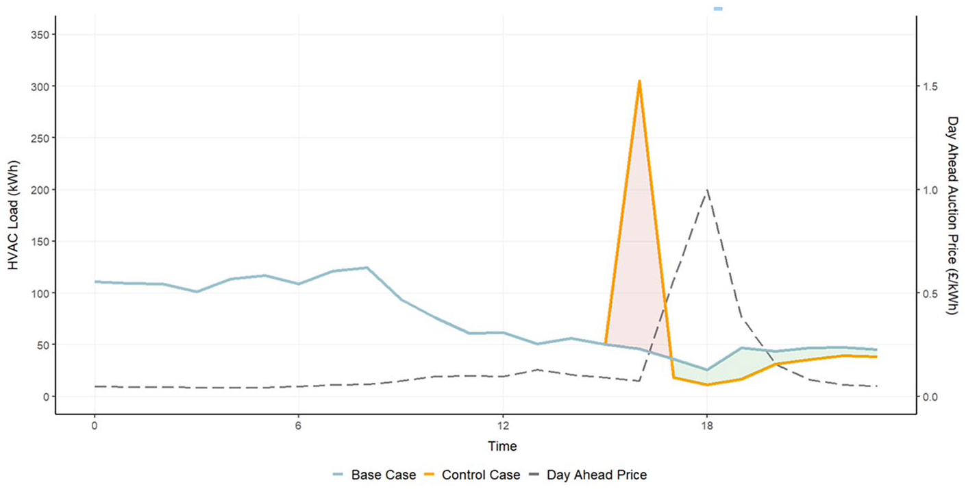
The cases outlined below show instances in which an arbitrage opportunity has been detected and is profitable. The model is run, a first time, to determine the hourly energy consumption based on the environmental conditions on that day. This base case sets the benchmark for the unaltered energy consumption, meaning that the energy consumed at any hour will be paid at the corresponding hourly rate. Before running the second simulation, the thermostat schedule is altered, such that the building is preconditioned ahead of the predetermined arbitrage opportunity. The second simulation is run providing a control case with a “charge” and “discharge” period. In the following figures, base cases and control cases are displayed by blue and orange solid lines respectively, while prices are represented by dashed lines; “charging” periods are shaded in red, and “discharging” periods are shaded in green.

14 January 2021—Heating with High Storage Capacity and Humidification

The day-ahead prices from 14 January 2021 displayed a price spread factor of 9.60x between 16:00 to 16:59, and 17:00 to 19:59. In a typical year, the base HVAC consumption, that is, potential spare capacity, between the latter period was of 95 kWh. This generous price differential and the potential spare capacity presented a promising arbitrage opportunity.

Three cases have been investigated. The first one looks into energy storage through preheating the building. The second case looks into pre-humidifying internal spaces. The final case combines both storage mediums.

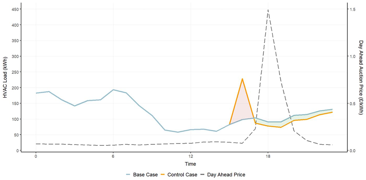
(i) Heating with High Storage Capacity Case

The Profit from this activity was a 33.76 percent of the baseline day’s cost. This is an exemplary case of day-ahead price arbitrage, as both storage capacity and price differential are large enough to produce a considerable profit (Figure 6).

Figure 6.

Heating with high storage capacity case—14 January 2021.

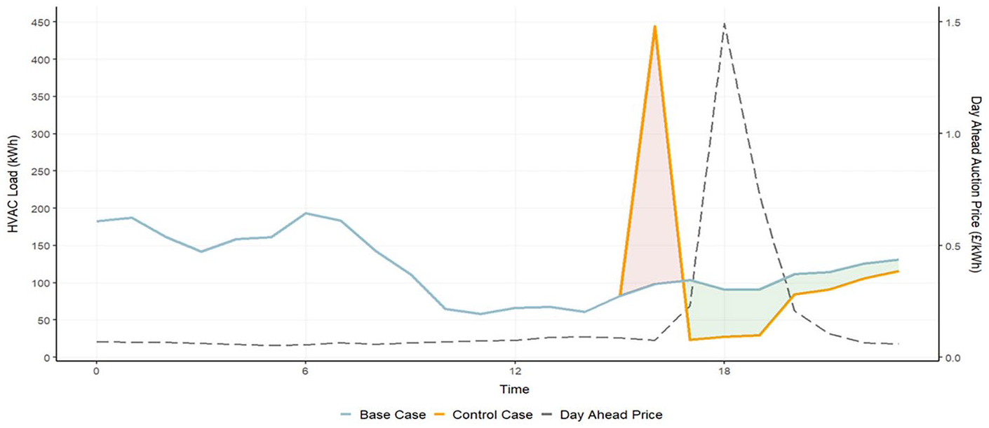
(ii) Humidification Case

The Profit from this activity was a 7.86 percent of the baseline day’s cost. During this service period, relative humidity in the base case was at the lower bound (35%). Thus, it was assumed that energy could also be stored in the form of humidity, thereby offsetting the need to consume electricity to humidify the air during the service period. An optimal case for this day-ahead price profile (Figure 7) was found when the relative humidity set-point was increased to 42 percent from 16:00 to 16:59.

Figure 7.

Humidification case—14 January 2021.

(iii) Combined Heating and Humidification Case

The Profit from this activity was a 31.80 percent of the baseline day’s cost. Although it may have been expected that merging the two strategies would inflate profits, the combined case shown in Figure 8 (thermostat setting at 23.5°C, and relative humidity set-point at 42%) does not attain the same cost reduction as the pure heating case. Savings were nearly two percentages points below the heating case. This can be explained by the inverse relationship between humidity and temperature. When the thermostat set-point is increased to 23.5°C, the humidifier increases the water content in the air to prevent relative humidity from plummeting below the 35 percent limit. Though the water content remains the same over the service period, the decaying air temperature drives relative humidity up. In this case, relative humidity reaches 42 percent, thereby making the use of a humidifier detrimental.

Figure 8.

Combined heating and humidification—14 January 2021.

6 January 2021—Heating with Low Storage Capacity

Instances of high price differentials can be observed in the auction prices. Usually, there is enough potential capacity in the HVAC system over the price differentials to exploit them. This case shows the opposite. Unlike the case above, which had an average potential capacity of around 95 kWh during the service period, the case shown in Figure 9 only has approximately 40 kW of average potential capacity. Nevertheless, the price spread factor is 7.65x and as a result the profit from this activity was a 11.56 percent of the baseline day’s cost. Relative humidity was already higher than the lower bound limit of 35 percent. Hence, the capacity for humidity storage over this service period is null.

Figure 9.

Heating with low storage capacity case—6 January 2021.

18 August 2019—Cooling

In contrast to the winter days, this case investigates the OSB’s ability to offset a price peak in a cooling month. Like the cases described above, preconditioning is used to achieve it, with the difference being that internal spaces are cooled, rather than heated. The inverse storage strategy is therefore used: the thermostat set-point is lowered from its default (24°C) to 20°C during the hour leading up to the price peak, then raised to 24.5°C during three hours before returning to the default set-point. Both HVAC loads and prices are, on average, low in cooling months, driving down the daily running costs. Prices are also lower when compared to heating months. Hence, absolute cost savings tend to be lower even though they may be proportionally significant. Nevertheless, reflected by the case shown in Figure 10, 7.52 percent savings on the day’s baseline cost could be achieved.

Figure 10.

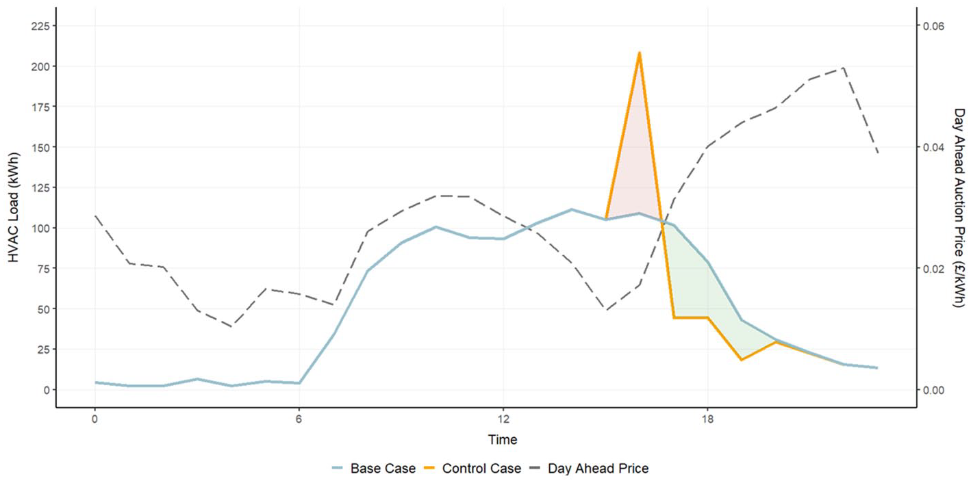
Cooling case—18 August 2019.

29 June 2020—Negative Day-Ahead Prices

On summer days when excess renewable generation leads to negative day-ahead prices, the gains are two-fold. Firstly, the OSB is being paid for consuming during these periods. Secondly, the HVAC consumption during subsequent positive prices can be offset by the storage strategy. These two effects combined can result in substantial cost reduction, both in relative and absolute terms. Thus, in Figure 11, day-ahead prices are shown to fall below zero between 3:00 and 6:59. Since it is a cooling month, the thermostat was lowered to 20°C during these times, leading to 24.41 percent profit on the day’s costs.

Figure 11.

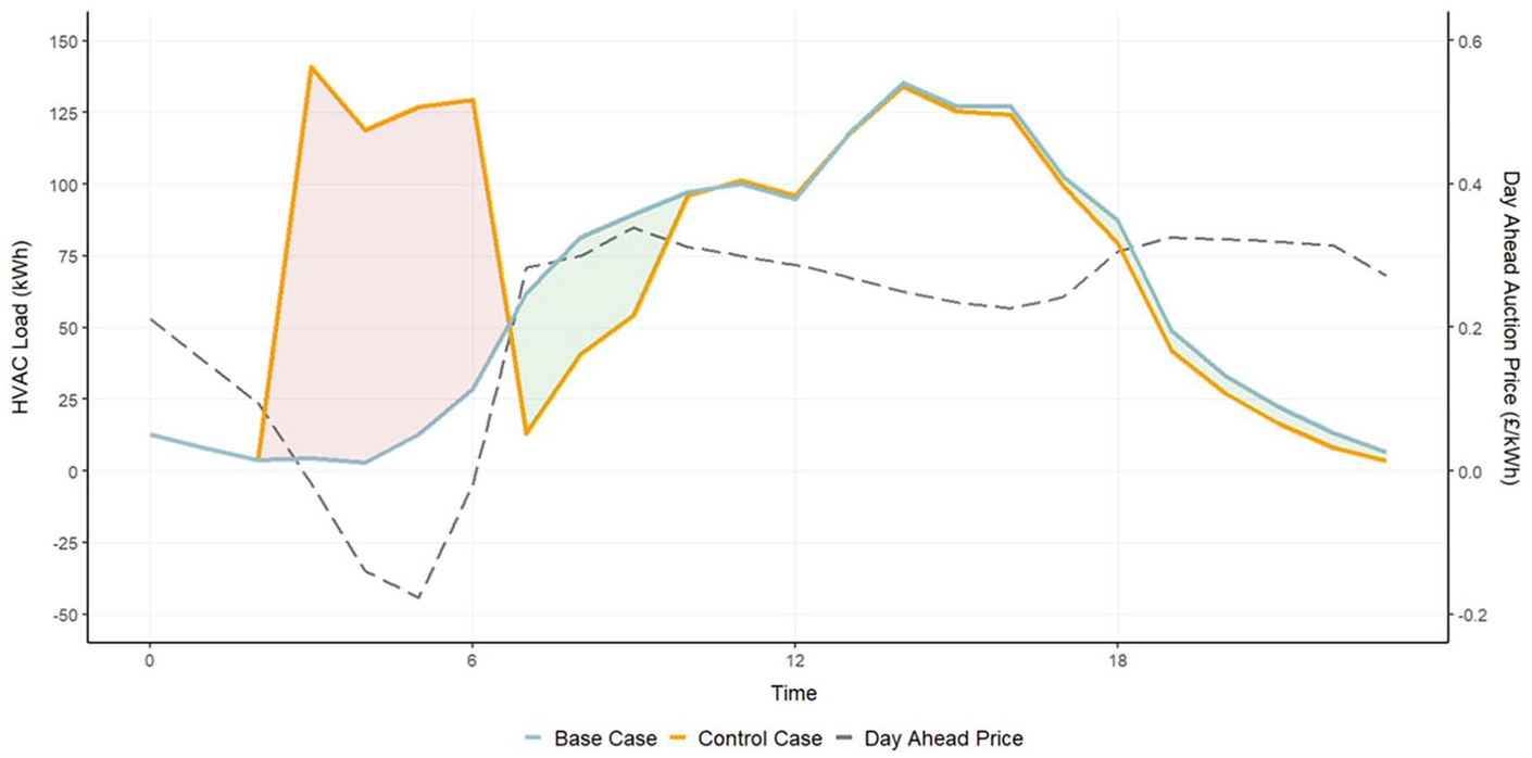
Negative day-ahead prices case—29 June 2020.

Overall, it is evident that a variety of opportunities arise throughout the year for substantial profits on the daily costs of energy by taking advantage of storage arbitrage opportunities. The actual amounts will depend upon the market prices and weather conditions. Indeed, the price spreads in 2022 were much higher than those examined in the above cases. Though price arbitrage opportunities are sporadic in the day-ahead market, they present no extra overhead and minimal additional complexity to energy management systems that would be purchasing power and scheduling HVAC systems anyway. Being alert to arbitrage storage opportunities is simply a smart extension of active energy management. Nevertheless, the larger arbitrage opportunities in this data were mainly in the winter months. For that reason, contracting for an alternative revenue stream from the network operators by offering reserve services may be more attractive.

5. Reserve Services Proof of Concept

Reserves are contracted by the network operators to ensure enough capacity is available throughout the day to be called in real time to balance the system. Capacity providers tender for specific service periods. Once the bid is accepted, depending on the electrical loads, the grid system operator may call upon as much of these contracted reserves as necessary. Sometimes referred to as a flexibility services, these reserves are fast-acting to cope with rapid mismatches, either positive or negative, in the demand and supply balance in real-time. In many markets, like GB, there are two levels of system operator: a national system operator who manages the high voltage national transmission system and local system operators who ensure the stability of the local distribution networks; both may contract for reserve services. Thus, in GB, the national transmission system operator (NESO), and for London local distribution, UK Power Networks (UKPN), each manage their own reserve requirements. NESO offers a day-ahead auction for Short Term Operating Reserve (STOR) to provide reserves at twenty minutes notice (National Grid ESO 2022). UKPN’s “Secure” flexibility programme consists of two annual auctions, one before the summer season (usually 1 June–30 August) and another before the winter season (usually 1 December–28 February). The capacity provider specifies the days of the week, and the times of the days, over which it can provide the reserve capacity during the entire season (UK Power Networks 2021). In each case, two prices must be tendered: the availability price, reflecting the opportunity cost to the provider of saving the contracted capacity for the grid, and the utilization price reflecting the cost to the provider of supplying the requested capacity as needed by the grid. Evidently these services are effectively call options by the system operators.

STOR may be more difficult to implement as the OSB’s thermal mass does not warm up enough in twenty minutes in order to meet the minimum service period of two hours (National Grid ESO 2022). On the contrary, higher degree of programmability offered by UKPN Secure allows the OSB to charge in winter mornings, when prices tend to be lowest, and storage capacity highest. Secure auction prices from the past three auctions (2018/2019, 2020/2021, 2021/2022) have been used to quantify potential cost reductions. The data has been refined to obtain a more realistic bidding scenario. Only winter bids have been selected, as the OSB’s low capacity during summer months does not allow continuous storage capacity. Finally, only accepted bids and accepted alternative efficient price offers (counter offers made by UKPN to certain tenders) have been included in the analysis. Table 3 shows the statistics from the resulting dataset.

Table 3.

UKPN Secure Auction Prices.

Year	UKPN availability (£/MWh)				UKPN utilization (£/MWh)
Year	Minimum	Maximum	Mean	SD	Minimum	Maximum	Mean	SD.
2018	0.00	465.00	80.34	115.91	0.00	1,275.50	341.93	369.79
2020	2.66	5,500.00	469.94	1,075.07	0.00	5,832.85	634.49	1,236.88
2021	3.00	1,480.00	258.78	289.30	17.00	7,561.00	368.81	695.00
All	0.00	5,500.00	307.28	649.34	0.00	7,561.00	448.32	887.66

The financial feasibility of the Secure programme was determined by comparing the electricity costs from a typical year without the programme (the base case), against one with the Secure programme (control case). It is assumed that the aggregator would procure all electricity from the day-ahead market. A detailed analysis of the HVAC loads in winter across all potential three-hour market opportunity windows revealed that between 6:00 and 9:00 would have the highest probability of providing most capacity. Thus, the base case’s electricity cost was calculated by multiplying the hourly base HVAC load of a typical winter season by the average wholesale price at each hour. For the control case, the optimal storage strategy was programmed at every day of the winter season, with the procurement period spanning between 5:00 and 5:59 and the service period between 6:00 and 8:59. The resulting HVAC load was multiplied by the same average wholesale price. Hence, the profit from each flexibility service $P_{φ}$ was given by the following equation:

\begin{matrix} P_{φ} = R_{F S} - C_{σ} \\ P_{φ, D a i l y} = \sum (λ_{A}^{F S} \times V_{F, t} + λ_{U}^{F S} \times V_{F, t} \times γ_{t}) - λ_{σ, c}^{D A} \times V_{σ, c} \\ P_{φ, S e a s o n a l} = \sum (λ_{A}^{F S} \times V_{F, t} + λ_{U}^{F S} \times V_{F, t} \times γ_{t}) - \sum (λ_{σ, c}^{D A} \times V_{σ, c}) \end{matrix}

Where: $λ_{A}^{F S}$ is the contracted availability price for the flexibility service

$V_{F, t}$ is the freed volume for the flexibility service at time $t$

$λ_{U}^{F S}$ is the contracted utilization price for the flexibility service

$γ_{F, t}$ is the utilization factor (proportion of freed capacity requested) at $t$

$λ_{σ, c}^{D A}$ is the day-ahead price at time $c$ during the procurement period $σ$

$V_{σ, c}$ is the volume traded at time $c$ during the procurement period $σ$

The analysis is subject to the sensitivity of two market variables: (i) the contracted availability price ( $λ_{A}^{F S}$ ), and (ii) the expected utilization revenue ( $λ_{U}^{F S} \times γ_{t} \sqrt$ ). The latter has been created to capture the fact that the reserves may be called upon at varying degrees. It is the product of the weighted average utilization factor across the season and the utilization price. This means that even though the utilization price may by £7.561/kWh, the utilization revenue at any time could be between zero and this value depending upon how much is called by the system operator. In general, bids from the UKPN Secure auction data are set for every day of the week, weekdays, or weekends (in order of frequency). Bids offering weekend capacity are infrequent. Bids also vary in length with most being up to four hours. Four example cases were produced. The first case was based on common bids, consisting of a three-hour (6:00–8:59), offering capacity every day of the week. In the second case, capacity is offer during weekdays during the same three-hour window. The third case is aimed at exploiting the subsequent reduction in HVAC consumption following the morning storage strategy by offering capacity over as much time as possible, that is, every day from 6:00 to 23:59. The final case takes the same approach as the third, but only for weekdays. Profits are provided relative to the base HVAC cost over the three months. We considered a wide range of variations for sensitivity analysis. The availability price has been varied according to the percentiles from the UKPN auction dataset, while the expected utilization revenue has been varied according to the percentiles from the contracted utilization fee. The full results are shown in the Appendix. We summarize the average values in Table 4.

Table 4.

Mean Net HVAC Load After Preconditioning.

Start time	End time	Mean net HVAC consumption—everyday (kWh)	Mean net HVAC consumption—weekdays (kWh)	Mean day-ahead price—everyday (£/kWh)	Mean day-ahead price—weekdays (£/kWh)
00:00	4:59	−31.4	−22.07	0.04101	0.04120
05:00	05:59	273.5	234.6	0.03526	0.03511
06:00	06:59	−84.8	−71.5	0.03961	0.03915
07:00	07:59	−69.0	−57.9	0.04715	0.04634
08:00	08:59	−55.0	−46.0	0.04850	0.04731
09:00	09:59	−18.4	−14.7	0.05322	0.05234
10:00	10:59	−13.7	−11.4	0.05605	0.05545
11:00	11:59	−10.5	−8.7	0.05506	0.05506
12:00	12:59	−9.1	−7.1	0.05363	0.05367
13:00	13:59	−8.1	−6.4	0.05493	0.05496
14:00	14:59	−7.6	−6.2	0.05326	0.05314
15:00	15:59	−7.4	−5.8	0.05104	0.05109
16:00	16:59	−8.0	−6.5	0.05005	0.05005
17:00	17:59	−7.9	−6.3	0.06767	0.06818
18:00	18:59	−7.7	−6.1	0.10325	0.09709
19:00	19:59	−7.7	−6.1	0.07667	0.07605
20:00	20:59	−7.3	−5.8	0.06163	0.06139
21:00	21:59	−7.2	−5.6	0.05203	0.05194
22:00	22:59	−7.1	−5.5	0.04843	0.04862
23:00	23:59	−7.0	−5.5	0.04324	0.04328
00:00	23:59	−101.5	−70.7	0.05232	0.05193

All cases show that offering flexibility to UKPN by using the proposed storage strategy is profitable for the OSB during a typical season, but the variation is huge. Seasonal profits have been predicted to range with a 750-fold difference between the lowest and highest. This range is a consequence of the vast differences in hours in operation (8.4-fold difference between largest and smallest) and the flexibility fees. Furthermore, it might be expected that when availability and factored utilization fees are zero, the HVAC consumption in the base case would equal that of the control case, that is, £10,100. Yet all cases show that, by default, undertaking the storage strategy is 7.9 percent (for every-day flexibility), or 5.3 percent (for weekday flexibility) less costly than the base case. The explanation for this can be seen through the data in Table 4, which shows that regularly preconditioning the building lowers the HVAC of preceding hours. Moreover, the difference in the default performance between the two control cases can be associated to the lack of preconditioning during weekends in the weekday case, as mean day-ahead prices and the proportional decrease in mean HVAC load are similar for both cases.

Profits can be achieved in all the cases outlined above, as shown in Table 5. As expected, the profit is positively correlated with the window length. The same cannot be said when examining total hours in operation per season. The profit rates illustrate that operating during weekdays is marginally less efficient than operating during the entire week. As mentioned, above, this cannot be due to disparity in weekend prices as both mean day-ahead price profiles are approximately the same. Instead, it is believed that it is related to the OSB’s thermodynamics. When the building is consistently preconditioned all week, the thermal mass remains above the 19°C. Hence, the thermal inertia continuously alleviates a small portion of the load after the three-hour period. When preconditioning ceases during weekends, the thermal mass returns to 19°C, effectively resetting the relative thermal inertia. This inertia then takes time and energy to return to the pre-weekend levels and is therefore unable to alleviate the HVAC load. The breakeven fees, or the weighted average service fees, are shown to be directly correlated with the hours in operation per season, yet inversely proportional the contracted availability and utilization fee percentiles. Thus, there is a higher probability of bids being accepted for eighteen-hour windows, as the aggregator can bid at lower prices.

Table 5.

Profit Rates with the Highest Flexibility Fees and Breakeven Fees for Each Case.

Timing	Hours per season (h)	Maximum Profit (£)	Profit rate (£/hr)	Breakeven fee (£/kWh)	Availability percentile	Utilization percentile
Weekly peak	270	£246,214	912	0.4953	83rd	83rd
Weekdays peak	193	£174,595	905	0.7175	92nd	92nd
Weekly longer	1,620	£404,615	250	0.3010	70th	52nd
Weekdays longer	1,157	£284,517	246	0.4397	76th	71st

Overall, it is uncertain which flexibility strategy is optimal, the three or eighteen-hour one. Since preconditioning starts in the morning, a three-hour strategy would allow the OSB to also trade in the wholesale during the evening. The eighteen-hour strategy maximizes the offset HVAC capacity more effectively, leading to around double the profit for larger utilization and availability fees. The root of this uncertainty lies in the prediction of the utilization factors. Nevertheless, the profits show that there is potential for thermal mass to be used as an effective storage medium in providing real-time flexibility reserve services to the distribution network and that these may be more profitable than seeking day-ahead arbitrage on the power exchange. They are also less risky than the arbitrage opportunities, as they provide contract fees as well as the utilization payments. Going forward, the regulatory context is favorable for the growth of flexibility markets with the UK regulatory body establishing a new Flexibility Market Operator to harmonize the service nationally and provide greater liquidity (Ofgem 2023).

6. Summary and Conclusion

A state-of-the-art architectural simulator was used to design a typical high-rise residential building in London and capture the thermodynamics of its hourly occupancy. The building was operated as a virtual battery by manipulating the HVAC set-points when a market opportunity was detected. The optimal storage strategy, which was established empirically, was employed during these market opportunities in order to reduce the HVAC system’s running costs. It was assumed that a market aggregator would be collaborating with an advanced energy service system to facilitate access to the wholesale electricity market.

Two potential markets were found to be profitable: price arbitrage on the electricity wholesale market and contracting with the local distribution network (UKPN) for flexible reserve services. The former aimed at minimizing consumption during daily price peaks, while the latter focussed on providing short term flexibility for London’s local distribution operator.

Various case studies regarding price arbitrage displayed a wide range of profits depending upon weather conditions and market prices. Cooling months were found to yield lower profit opportunities, due to smaller, more volatile HVAC loads. Humidity was discovered to be far less frequent and effective at storing energy than the thermal mass. Despite the substantial arbitrage profits on favorable days, not every day presents these opportunities and so there would be considerable uncertainty, ex ante, on what to expect from an annual arbitrage policy⁴ in this respect. Compared to the arbitrage trading, the flexibility reserve services offered by UKPN to contract in advance and schedule the trading days and windows removes the uncertainty found in arbitrage trading. Moreover, the accepted utilization and availability fees were far larger than the price differentials observed in the day-ahead power exchange, for this period of data.

For the purpose of proving the concept of buildings as batteries, the weather of a “typical year” was fed into the simulations. The TRY dataset dampens the effects of extreme and erratic meteorological patterns, which will impact the energy consumption profile of a building. However, in practice building administrators trading in the day ahead market will benefit from more accurate weather forecasts. Scenario-based testing with varying weather profiles could be conducted to understand the meteorological risks of longer-term schemes, such as the UKPN Secure programme.

The architectural configuration and thermal properties of buildings can greatly affect their thermodynamic behavior. Most of the UK’s housing stock is composed of terraced, detached, or semi-detached properties, which, unlike high-rise buildings, do not benefit from large thermal masses. Also, they are typically older than high-rise buildings, and therefore have lower thermal insulation. These two factors are crucial in operating a building as a battery, making this study exclusive to high-rise buildings. Further research is required to understand the feasibility of operating other buildings types as batteries. In practice, building administrators would need to overcome a range of constraints posed by the individual needs of the residents. An evident one would be residents opting out of the trading schemes at any point in time. Additionally, residents may resort to heating or cooling their properties, thereby impacting the available capacity profile throughout the day. Operational reliability, such as HVAC malfunctions, must also be assessed.

Results would be different for varying geographical and jurisdictional locations. Although buildings located in more extreme climates, may benefit from higher tradeable power capacities throughout the year, London’s liberalized trading and regulations favor innovative business models by aggregators. Whilst the experimental design, using an architectural simulator inevitably abstracts from reality, the software has high credibility in practice. The simulation approach allows consistent counterfactuals to be referenced, which would be elusive to estimate from real building data where live experiments have not been conducted. Although it is hard to generalize in quantitative terms from the specificities of this study, we consider it offers a strong indication that active management of a building’s thermal inertia would be a useful addition to an aggregator’s portfolio of resources and one that involves relatively little investment other than modified ICT systems.

Finally, as with all storage technologies and arbitrage opportunities, the benefits become eroded with greater participation, but the nature of the energy transition suggests a growing need for many types of storage. Renewable technologies impose increasing requirements on the system for storage and it is likely that the growth of this requirement may be faster than its saturation of supply. If that is the case, the indications in this study of the potential role that buildings can provide within an aggregator’s portfolio of local energy resources may be an underestimate.

Footnotes

Appendix

The sensitivity results for the UKPN Secure service profits are shown in the following Tables based upon the percentiles of the utilization and availability costs.

Declaration of Conflicting Interests

The author(s) declared no potential conflicts of interest with respect to the research, authorship, and/or publication of this article.

Funding

The author(s) received no financial support for the research, authorship, and/or publication of this article.

Notes

References

Abramova

Bunn

2019. “Estimating Dynamic Conditional Spread Densities to Optimise Daily Storage Trading of Electricity.” https://ssrn.com/abstract=3349105.

Amasyali

El-Gohary

N. M.

2018. “A Review of Data-Driven Building Energy Consumption Prediction Studies. Renewable and Sustainable Energy Reviews 81: 1192–205.

Arcos-Vargas

Á.

Canca

Núñez

2020. “Impact of Battery Technological Progress on Electricity Arbitrage: An Application to the Iberian Market.” Applied Energy 260: 114273.

ASHRAE. 2001. ASHRAE Handbook: Fundamentals. Atlanta, GA: ASHRAE.

ASHRAE. 2010. Standard 55-2010: Thermal Environmental Conditions for Human Occupancy, Atlanta, GA: ASHRAE.

ASHRAE. 2016. Standard 62.1-2016: Ventilation for Acceptable Indoor Air Quality, Atlanta, GA: ASHRAE.

Bishop

J. D.

Axon

C. J.

Bonilla

Banister

2016. “Estimating the Grid Payments Necessary to Compensate Additional Costs to Prospective Electric Vehicle Owners Who Provide Vehicle-to-Grid Ancillary Services.” Energy 94: 715–27.

BSI British Standard. 2022. BS EN 14511-2022: Air Conditioners, Liquid Chilling Packages and Heat Pumps for Space Heating and Cooling and Process Chillers, with Electrically Driven Compressors. British Standard. https://www.en-standard.eu/

Burger

Chaves-Ávila

J. P.

Batlle

Pérez-Arriaga

I. J.

2016. The Value of Aggregators in Electricity Systems. Cambridge, MA: MIT Center for Energy and Environmental Policy Research.

10.

CIBSE. 2016. “CIBSE Weather Data Sets.” [Online]. https://www.cibse.org/media/fxzgxqy4/weath-data-sets-packages-only_1.pdf

11.

Cole

W. J.

Powell

K. M.

Hale

E. T.

Edgar

T. F.

2014. “Reduced-Order Residential Home Modeling for Model Predictive Control.” Energy and Buildings 74: 69–77.

12.

Dudley

J. H.

Black

Apte

Piette

M. A.

2010. Comparison of Demand Response Performance with an EnergyPlus Model in a Low Energy Campus Building. Lawrence Berkley National Laboratory.

13.

EU. 2017. Electricity Balancing Guideline https://eur-lex.europa.eu/legal-content/EN/TXT/?uri=CELEX:02017R2195-20210315

14.

Elexon. 2022. System price analysis report archive. https://www.elexon.co.uk/data/system-prices-analysisreport/spar-archive/https://www.elexon.co.uk/

15.

Eunomia. 2016. Investing in UK Electricity Storage. Bristol, UK: Eunomia.

16.

Farzana

Liu

Baldwin

Hossain

2014. “Prediction of Building Energy Consumption by Using Artificial Neural Networks.” Energy and Buildings 81: 161–9.

17.

FERC. 2020. Participation of distributed energy resource aggregations in markets operated by regional transmission organizations and independent system operators. https://www.federalregister.gov/documents/2021/03/30/2021-06089/participation-of-distributedenergy-resource-aggregations-in-markets-operated-by-regional/https://www.federalregister.gov/

18.

Ferlito

Atrigna

Graditi

De Vito

Salvato

Buonanno

Di Francia

2015. Predictive Models for Building’s Energy Consumption: An Artificial Neural Network (ANN) Approach. Trento, Italy: Institute of Electrical and Electronics Engineers.

19.

Frate

G. F.

Ferrari

Desideri

2021. “Energy Storage for Grid-Scale Applications: Technology Review and Economic Feasibility Analysis.” Renewable Energy 163: 1754–72.

20.

Giuletti

Grossi

Buate

E.T.

Waterson

2018. Analyzing the potential economic value of energy storage. The Energy Journal 39 (SI1): 101–22

21.

GLA. 2016. Housing: Supplementary Planning Guidance. London, UK: Greater London Authority.

22.

Godina

Rodrigues

E. M. G.

Pouresmaeil

Matias

J. C. O.

Catalão

J. P. S.

2018. “Model Predictive Control Home Energy Management and Optimization Strategy with Demand Response.” Applied Sciences 8 (3): 408.

23.

Goia

2016. “Search for the Optimal Window-to-Wall Ratio in Office Buildings in Different European Climates and the Implications on Total Energy Saving Potential.” Solar Energy 132: 467–92.

24.

HCA. 2015. Employment Density Guide. London, UK: UK Homes & Communities Agency.

25.

Heidari-Rarani

Aliha

Sokrieh

Ayatollahi

2014. “Mechanical Durability of an Optimized Polymer Concrete Under Various Thermal Cyclic Loadings: An Experimental Study.” Construction and Building Materials 64: 308–15.

26.

Huang

Chen

2014. Model Predictive Control for Energy-Efficient Buildings: An Airport Terminal Building Study. Taichung, Taiwan: Institute of Electrical and Electronics Engineers.

27.

IRENA. 2019. Innovation Landscape for a Renewable-Powered Future: Solutions to Integrate Variable Renewables. Abu Dhabi: International Renewable Energy Agency.

28.

Jin

Jia

Jiang

2017. “Dynamic Economic Dispatch of a Hybrid Energy Microgrid Considering Building Based Virtual Energy Storage System.” Applied Energy 194: 386–98.

29.

Joe

Dong

Munk

Kuruganti

Cui

2020. “Virtual Storage Capability of Residential Buildings for Sustainable Smart City via Model-Based Predictive Control.” Sustainable Cities and Society 64: 102491.

30.

Johra

Heiselberg

Le Dréau

2019. “Influence of Envelope, Structural Thermal Mass and Indoor Content on the Building Heating Energy Flexibility.” Energy and Building 183: 325–39.

31.

Lazard. 2021. Lazard’s levelized Cost of Storage Analysis—Version 7.0. Hamilton, Bermuda: Lazard.

32.

Le Dréau

Heiselber

2016. “Energy Flexibility of Residential Buildings Using Short Term Heat Storage in the Thermal Mass.” Energy 111: 991–1002.

33.

Makibar Puente

Navarte Fernández

2015. “Characterisation and Efficiency Test of a Li-Ion Energy Storage System for PV Systems.” 31st European photovoltaic Solar Energy Conference and Exhibition, Hamburg, 1652–558.

34.

Massana

Colomer

2016. “Short-Term Load Forecasting for Non-Residential Buildings Contrasting Artificial Occupancy Attributes.” Energy and Buildings 130: 519–31.

35.

Mat Daut

M. A.

Hassan

M. Y.

Abdullah

Rahman

H. A.

Abdullah

M. P.

Hussin

2017. “Building Electrical Energy Consumption Forecasting Analysis Using Conventional and Artificial Intelligence Methods: A Review.” Renewable and Sustainable Energy Reviews 70: 1108–18.

36.

McKenna

McManus

Cooper

Thomason

2013. “Economic and Environmental Impact of Lead-Acid Batteries in Grid-Connected Domestic PV Systems.” Applied Energy 104: 239–49.

37.

Meng

Dong

Z. Y.

Zheng

Hill

D. J.

2019. “Coordinated Dispatch of Virtual Energy Storage Systems in Smart Distribution Networks for Loading Management.” IEEE Transactions on Systems 49 (4): 776–86.

38.

Metz

Saraiva

J. T.

2018. “Use of Battery Storage Systems for Price Arbitrage Operations in the 15- and 60-Min German Intraday Markets.” Electric Power Systems Research 160: 27–36.

39.

MHCLG. 2017. English Housing Survey. London, UK: UK Ministry of Housing, Communities & Local Government.

40.

National Grid ESO. 2022. “STOR—Technical Requirements.” [Online]. https://www.nationalgrideso.com/industry-information/balancing-services/Reserve-Services/Short-term-operating-reserve/Technical-Requirements.

41.

Ofgem. 2021. Review of GB Energy System Operation. London, UK: Ofgem.

42.

Ofgem. 2023. “Consultation: Market Facilitator Delivery Body.” https://www.ofgem.gov.uk/publications/consultation-market-facilitator-delivery-body.

43.

OpenStudio, 2022. “OpenStudio®.” [Online]. https://openstudio.net/.

44.

Paudel

Nguyen

Kling

W. L.

Elmitri

2015. Support Vector Machine in Prediction of Building Energy Demand Using Pseudo Dynamic Approach. Pau, France: Cornell University.

45.

Pereira da Silva

Paulo

2019. “The Effect of Variable Renewable Energy Sources on Electricity Price Volatility: The Case of the Iberian Market. International Journal of Sustainable Energy 38 (8): 794–813.

46.

Raman

N. S.

Barooah

2020. “On the Round-Trip Efficiency of an HVAC-Based Virtual Battery.” IEEE Transactions on Smart Grid 11: 403–10.

47.

Reilly

Kinnane

2017. “The Impact of Thermal Mass on Building Energy Consumption.” Applied Energy 198: 108–21.

48.

Rintamäki

Siddiqui

A. S.

Salo

2017. “Does Renewable Energy Generation Decrease the Volatility of Electricity Prices? An Analysis of Denmark and Germany.” Energy Economics 62: 270–82.

49.

Runge

Zmeureanu

2019. “Forecasting Energy Use in Buildings Using Artificial Neural Networks: A Review.” Energies 12 (17): 3254.

50.

Tesla. 2020. Tesla Powerwall 2 AC Datasheet—United Kingdom, Austin, TX: Tesla.

51.

UK Power Networks. 2021. Flexibility Services Procurement Statement. London: UK Power Networks.

52.

Vesterberg

Krishnamurthy

C. K. B.

2016. Residential end-use electricity demand: Implications for real time pricing in Sweden. The Energy Journal 37 (4): 141–64