Sage Journals: Discover world-class research

Abstract

Thyroid tissue is sensitive to the effects of endocrine disrupting substances, and this represents a significant health concern. Histopathological analysis of tissue sections of the rat thyroid gland remains the gold standard for the evaluation for agrochemical effects on the thyroid. However, there is a high degree of variability in the appearance of the rat thyroid gland, and toxicologic pathologists often struggle to decide on and consistently apply a threshold for recording low-grade thyroid follicular hypertrophy. This research project developed a deep learning image analysis solution that provides a quantitative score based on the morphological measurements of individual follicles that can be integrated into the standard pathology workflow. To achieve this, a U-Net convolutional deep learning neural network was used that not just identifies the various tissue components but also delineates individual follicles. Further steps to process the raw individual follicle data were developed using empirical models optimized to produce thyroid activity scores that were shown to be superior to the mean epithelial area approach when compared with pathologists’ scores. These scores can be used for pathologist decision support using appropriate statistical methods to assess the presence or absence of low-grade thyroid hypertrophy at the group level.

Keywords

thyroid follicular hypertrophy histopathology digital pathology image analysis deep learning neural networks empirical models

Introduction

The thyroid gland is an important organ of the endocrine system. Its normal function and hormone regulation are essential for many processes including metabolism, neuronal development, and reproductive function.^8,14 Thyroid tissue is very sensitive to the effects of endocrine disrupting substances and this represents a significant health concern.¹⁵

Thyroid follicles are the structural and functional units of the thyroid gland. Rats, particularly males, have a higher background level of thyroid activity than humans and most mammals. They are also more sensitive to chemical-induced effects as a consequence of several differences including shorter plasma half-life of thyroid hormones (THs) and reduced buffering capacity due to smaller colloid stores. Differences in thyroid-stimulating hormone (TSH) potency and differences in metabolic pathways also exist. In particular, excretion in the liver is primarily through glucuronidation in rats and sulfation in humans.⁹ The latter is significant as many chemicals induce glucuronidation enzymes in the liver (uridine diphosphate-glucuronosyltransferases) in rats leading to the combination of liver and thyroid hypertrophy commonly observed in short-term toxicity studies. This mechanism may be referred to as liver-mediated or indirect thyroid toxicity and tends to induce lower grade (minimal or mild) follicular cell hypertrophy, whereas direct thyroid toxicants, such as propyl thiouracil, may induce higher grades.²

Endocrine disruptors may affect thyroid function via actions on a multitude of targets in the hypothalamo-pituitary-thyroid axis²⁹ and this may result in changes in the thyroid including a decrease in follicle luminal size due to the depletion of colloid.⁴ The potential for endocrine disrupting substances to cause downregulation of TH production is an important concern, since insufficient supply of TH to the human fetus during pregnancy can lead to delayed fetal brain development or irreversible damage.¹⁹ Although iodine deficiency is the most common cause for insufficient THs, other factors such as exposure to environmental chemicals, for instance, pesticides, are gaining increasing attention.¹¹ The potential for endocrine disruption requires evaluation before an agrochemical can be placed on the market and various OECD guidelines for repeated dose toxicity studies require assessment of endocrine disrupting properties.¹

Histopathology analysis of tissue sections of the thyroid gland remains the gold standard for the evaluation for pharmaceutical or chemical effects on the thyroid, however, the judgment of the presence or absence of thyroid hypertrophy is a particular challenge in rats. There is a high degree of intra- and inter-animal variability in the appearance of individual thyroid follicles. The evaluating pathologist must consider the appearance of the thyroid gland section as a whole, which typically includes several hundred follicles, consolidate this information, and place each animal on a continuum with respect to the range of this variation. At the extremes, there is a clear distinction between a thyroid with very low activity and one with very high activity, unequivocally assigned a high-grade of follicular hypertrophy. However, a significant proportion of control thyroids, especially in male rats, appear unusually active and there is a potential overlap between such control thyroids and where the study pathologist might consider recording minimal hypertrophy. A pathologist evaluating a study must therefore consider where the threshold for recording hypertrophy should be and on which side of this threshold each individual animal should be placed. Maintaining consistency even within a study is challenging, and pathologists often use approaches such as blinded evaluation, secondary to a primary read, to ensure the same threshold is applied amongst groups and to differentiate background variation in controls versus true treatment-related changes in treated groups, and may choose to rank the thyroids and set the threshold at the level of the highest control.³ There will sometimes be inconsistency in where this threshold is placed, especially between studies and different pathologists.

The aim of this work was to develop a deep learning image analysis solution that will support the decision-making process when evaluating thyroid hypertrophy, particularly at the low-grade equivocal level. Conventional image analysis approaches involve setting a ground truth whereby human operators select samples with and without a lesion or delineate a lesion within a sample. An algorithm is developed to reproduce the human output as closely as possible. Whatever threshold is selected, there will always be a trade-off between specificity and sensitivity (avoiding false positives and negatives, respectively) and potentially important variation on either side of the threshold may not be accounted for. Therefore, our objective was not to create a process that makes a judgment on the presence or absence of hypertrophy in each animal, but to generate a quantitative output that can be used to compare treatment groups against control groups statistically. Various approaches to produce this quantitative output are compared in this article.

Our process involves the acquisition of individual follicle measurements using a deep learning algorithm, that not just identifies the various tissue components but also delineates individual follicles by separating adjacent follicles and includes only intact follicles. It is vital to demonstrate that the data generated are representative of the way human observers perceive the variation in microscopic appearance in different samples. To achieve this, we applied the method of subjective ranking. Pathologists evaluated batches of thyroids and were asked to rank them in order (from high to low), as opposed to assigning them to discrete categories. This yields far more data on which to develop and validate the performance of various calculations and models, as variation within such categories are captured. It also avoids the need to align the thresholds between different observers. Subjective ranking is used commonly in a wide range of disciplines in situations where it is relatively easy for an observer to decide if one subject scores higher, lower or the same as another, but much harder to assign an actual value that can be consistently applied. Giles et al¹² explain this in their introduction and use the example of a test driver comparing how a car performs with different suspension set ups.

Correlation of the various quantitative methods to the pathologists’ scores obtained by subjective ranking was quantified using regression analysis. Improvements over simple calculations can be potentially achieved by applying empirical modeling methods. An empirical model, sometimes called a statistical model, relies on observation rather than theory. Empirical modeling involves collecting experimental data for the dependent and independent variables of a model, then uses a mathematical procedure to determine the parameter values that give the best fit for the data.²⁰ We hypothesized that certain morphological features of follicles (eg, mean diameter or epithelial thickness) are interpreted by pathologists such that some follicle morphologies are more predictive of the presence, or conversely absence, of hypertrophy, whereas others yield little information and are little more than noise. Based on this, we developed empirical models that adjusted raw individual follicle measurements (the dependent variables) to produce quantitative outputs optimized to align with the pathologists’ scores derived from subjective ranking (the independent variables). In this article, we compare the performance of these models against each other and against methods based on fixed calculations.

Materials and Methods

Training and Test Material

All material selected for inclusion in this project was obtained from nonclinical safety assessment studies in the rat (Han Wistar) that were previously conducted by CRL Edinburgh, on behalf of Syngenta Ltd., in accordance with study plans, the principles of Good Laboratory Practice and local legislation for conducting scientific procedures on animals, ie, the UK Home Office Legislation (Animals [Scientific Procedures] 1986 Act, which conforms to the European Convention for the Protection of Vertebrate Animals Used for Experimental or Other Scientific Purposes (Strasburg, Council of Europe)) and approved by the Animal Experimental Ethics Committee of CRL Edinburgh. The tissue examined in all cases was formalin-fixed, paraffin embedded, thyroid gland from repeat dose dietary administration studies (28 and 90-day studies), processed histologically according to internal standard operating procedures.

Image Analysis (IA)

Hematoxylin and eosin (H&E) stained thyroid gland slides were anonymized and scanned using a Leica Aperio AT2 slide scanner at x40 objective magnification at a resolution of 0.25 microns/pixel. Whole Slide Images (WSIs) were imported into Visiopharm software (version no. 2022.01) for image analysis. Training was performed by an image analysis scientist who had received training on the microscopic anatomy of the thyroid gland and under the supervision of boarded veterinary pathologists. A total of 107 training regions of interest (ROI) were selected from the 62 WSIs of different male and female rats from 28- and 90-day studies. Slides selected for training purposes were chosen to represent a mix of control and mild or minimal hypertrophy with as wide a variety in staining intensity and tissue morphology as possible. Both small (2 to 3 follicles) and large (10 plus follicles plus background tissue) ROIs were selected within the training slides and their locations covered all areas of the gland and were chosen to provide a diverse range of the objects of interest. In total, an area equaling 40.61 mm² of thyroid tissue was used for training.

Algorithm Development

A tissue detection algorithm (Bayesian linear) was developed to initially segment tissue from background based on thresholding parameters. Each slide contained paired thyroid sections which were given unique identifiers during the tissue detection step.

Follicle recognition algorithm—IA model 1

A follicle recognition algorithm was created to specifically detect intact follicles, defined as colloid surrounded by a complete follicular cell layer. A deep learning classifier was trained to detect three classes within the thyroid gland: background structures; follicular cell layer; and colloid. Background structures consisted of brown and white adipose tissue, loose connective tissue, C-cells and follicular cells from follicles out of plane of section, skeletal muscle, blood vessels, hemorrhage, parathyroid glandular tissue, lymphoid aggregates and follicular cysts, and were excluded from further analysis. During ground-truth annotations, conducted by image analysis scientists trained by boarded pathologists, accurate labeling of the outer limit of the follicular cell layer was a particular challenge. To maintain consistency between follicles/parts of follicles in which the basement membrane was clearly defined and those in which no outer margin was evident, annotations followed the basal margins of the follicular cell nuclei. Segmentation of the colloid was easily performed due to the clear demarcation of colloid from the follicular cell layer.

A U-Net convolutional deep learning neural network was trained on manually drawn or corrected labels within ROIs within the detected tissue. The algorithm was subjected to 700,000 training iterations. A total of 56 additional post processing steps were included to correct small areas of misdetection and to identify and separate adjacent follicles that had been detected as a single entity. Finally, colloid or follicular cell layers that were detected in isolation were removed to leave only intact follicles. XY coordinates were generated for each follicle to facilitate the visual examination of individual follicles for quality control purposes and to enable evaluation of the algorithm performance on individual outlier follicles. The raw output of the algorithm was expressed as area of colloid label in µm², perimeter of colloid label in µm, area of follicular cell layer label in µm² and outer perimeter of follicular cell layer label in µm. Established formulae for the area and perimeter of an ellipse²⁶ were used to convert the raw data outputs into mean epithelial height and mean follicle diameter of each follicle, taking into account deviations from the roundness, considered to be more intuitive when graphically presented, and therefore facilitate development of empirical models.

Mean epithelial area algorithm—IA model 2

Two further algorithms were created to calculate the Mean Epithelial Area. An initial algorithm was developed to identify three classes within the thyroid gland: background structures; follicular cells/C-cells; and colloid. Unlike in the IA model 1, follicular cells detected included both cells in clearly defined layers and those belonging to partially transected follicles out of plane of section. The background structures and colloid were excluded from further analysis. The remaining follicular cells/C-cells were isolated as a single ROI. A second algorithm was developed to detect cell nuclei within the follicular cell layer ROI. A U-Net convolution deep learning neural network was trained on manually drawn labels with the final algorithm being subjected to 200,000 training iterations. A total of eight additional postprocessing steps was included to correct any minor areas of misdetection. The output of the two steps used in this process are expressed as follicular cell area (µm²) and total number of nuclei identified within the follicular cell area ROI. Division of follicular cell/C-cell area by total nuclei number generated the mean epithelial area.

Data, from both IA models, were exported from Visiopharm software into Microsoft Excel spreadsheets.

Methods to Calculate Thyroid Activity Scores

Various fixed calculation methods and empirical models were developed to process the output variables of the IA model 1. For model development, agrochemical studies of 90-days duration in which minimal or mild thyroid hypertrophy had been previously diagnosed were selected (referred to as development studies 1 and 2). The output from these models was a single value referred to subsequently as the thyroid activity score (TAS).

For comparison, a pathologist reference standard was generated based on subjective ranking. Four pathologists (each with at least 10-years of experience in toxicologic pathology) blind read 30 slides (10 controls, 10 intermediate and 10 high dose animals) of each sex from both development studies and ranked each animal in order of perceived thyroid activity. Each animal was assigned a relative rank within a cohort, grouping indistinguishable animals and assigning the mid-interval rank to each when necessary, and the combined rank from each of the four pathologists was calculated to provide a single score for each animal. These are referred to throughout as the pathologists’ scores (Supplemental Tables 1-4).

Fixed calculation method 1 used the ratio of epithelial area to colloid area obtained from IA model 1 expressed as a mean, following adjustment with the area fraction of each follicle relative to the total area of all follicles. Fixed calculation method 2 used the mean epithelial area of all follicles obtained from IA model 2. Fixed calculation method 3 was created by the combination of the outputs of the other two fixed calculation methods, ie, multiplication of the two outputs followed by log transformation.

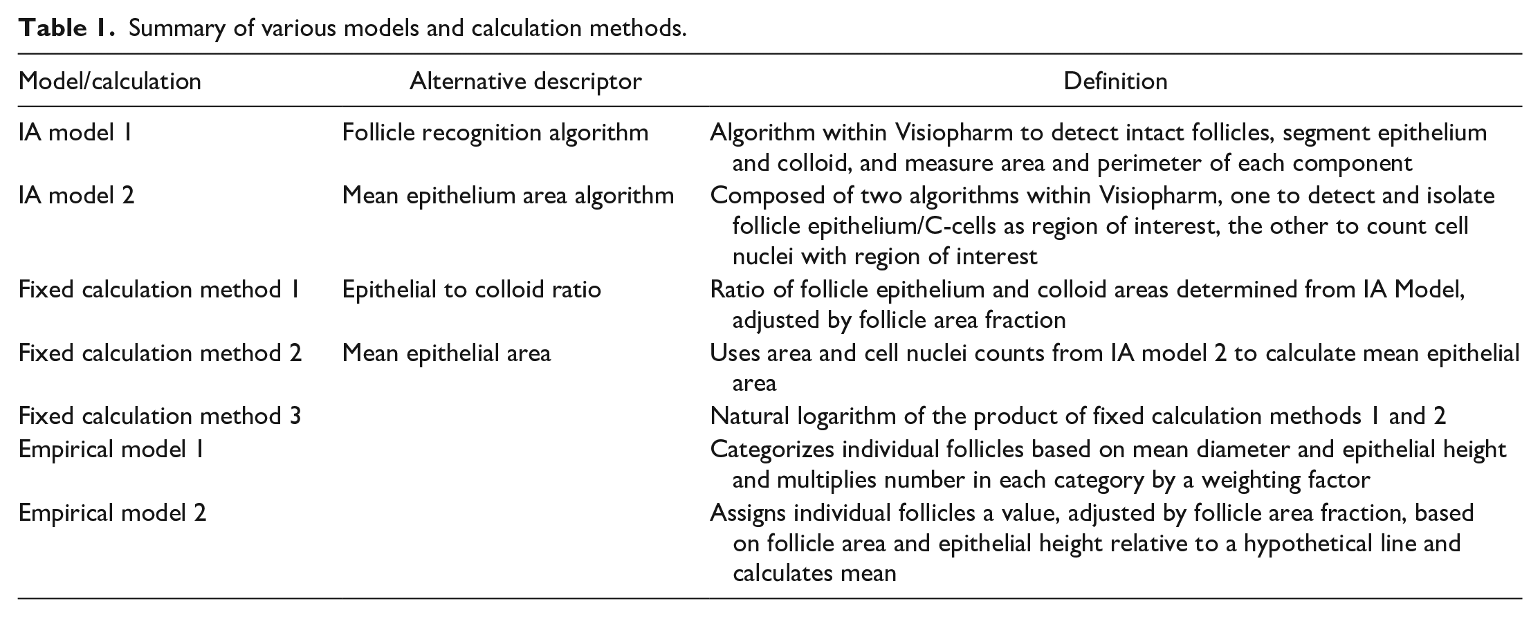
Various empirical models were developed and tested. The performance of these models, and the various fixed calculations, was determined by how well the output correlated with the pathologists’ scores using Pearson’s coefficient of determination (R²). Models for males and females were developed separately, but the output from each development study while training a specific model was displayed simultaneously. An iteration that yielded a good result in only one study was immediately rejected. Importantly, this approach ensured that a model was robust and not developed to fit just one set of training slides, ie, avoided overfitting to one set. Two empirical models were selected for potential use. Empirical model 1 categorized follicles based on mean follicle diameter and epithelial height. The number of follicles in each category was multiplied by a weighting factor and the TAS for each animal generated from the sum of all categories divided by the total number of follicles. The cut-off values between each category and the weighting factors were the random inputs for the model. Empirical model 2 assigned individual follicles a score based on their mean diameter and epithelial height. The distance above or below a hypothetical straight line described by a linear equation (ie, y = mx + c, where m and c are two of the random inputs for the model), adjusted with additional random inputs, dictated the score for each follicle. Follicles above the line were assigned a positive value and those below the line a negative value. The TAS for each animal was the mean follicle score, adjusted for area fraction. A summary of the various IA models, fixed calculations and empirical models is provided in Table 1.

Table 1.

Summary of various models and calculation methods.

Model/calculation	Alternative descriptor	Definition
IA model 1	Follicle recognition algorithm	Algorithm within Visiopharm to detect intact follicles, segment epithelium and colloid, and measure area and perimeter of each component
IA model 2	Mean epithelium area algorithm	Composed of two algorithms within Visiopharm, one to detect and isolate follicle epithelium/C-cells as region of interest, the other to count cell nuclei with region of interest
Fixed calculation method 1	Epithelial to colloid ratio	Ratio of follicle epithelium and colloid areas determined from IA Model, adjusted by follicle area fraction
Fixed calculation method 2	Mean epithelial area	Uses area and cell nuclei counts from IA model 2 to calculate mean epithelial area
Fixed calculation method 3		Natural logarithm of the product of fixed calculation methods 1 and 2
Empirical model 1		Categorizes individual follicles based on mean diameter and epithelial height and multiplies number in each category by a weighting factor
Empirical model 2		Assigns individual follicles a value, adjusted by follicle area fraction, based on follicle area and epithelial height relative to a hypothetical line and calculates mean

Statistics

To assess the overall degree of agreement between the pathologists generating the subjective ranking data, an inter-rater reliability (IRR) assessment known as the intraclass-correlation coefficient (ICC) was calculated for the pathologist’s subjective rankings of Studies 1 and 2 using a two-way, average measures, mixed effects model, applying consistency to assess good IRR.¹³ This was conducted in SAS²⁷ according to the method described by Maki.²¹

Pearson’s coefficient of determination R² was calculated within Microsoft Excel using the square of the Pearson’s correlation coefficient R (function “CORREL”). The R² provides a measure of how well observed outcomes are predicted by a model, based on the proportion of total variation of outcomes that can be explained by a model, relative to unexplained variability.^6,22,31 This value was used to assess the performance of each empirical model during their optimization, and also determined for the fixed calculations for comparison.

The two empirical models described above, and fixed calculation method 3, were applied to cohorts of one hundred controls specific to each sex and study duration (28 and 90 days) and tested for normality in SAS²⁷ using Shapiro-Wilk’s test.²⁸ They were also compared with each other on the same control data sets using R² to assess the risk of multicollinearity, relevant to the application of MANOVA.

Results

Image Analysis

Image analysis model 1 successfully identified follicular cell layers surrounding colloid. Incomplete follicular cell layers and other background structures defined in the methods were excluded from the analysis (Figure 1B). We were able to quantify a number of parameters, such as number of follicles per gland (Figure 2A), area of the follicular cell layer (Figure 2B) and the area of colloid detected per gland (Figure 2C). Image analysis model 2 identified and quantified total cellular area and the total number of nuclei within this specified area (Figure 1D, 2E). As well as cells in the follicular cell layer, this also included C-cells and follicular cells belonging to partially transected follicles out of plane of section (Figure 1C, 2D).

Figure 1.

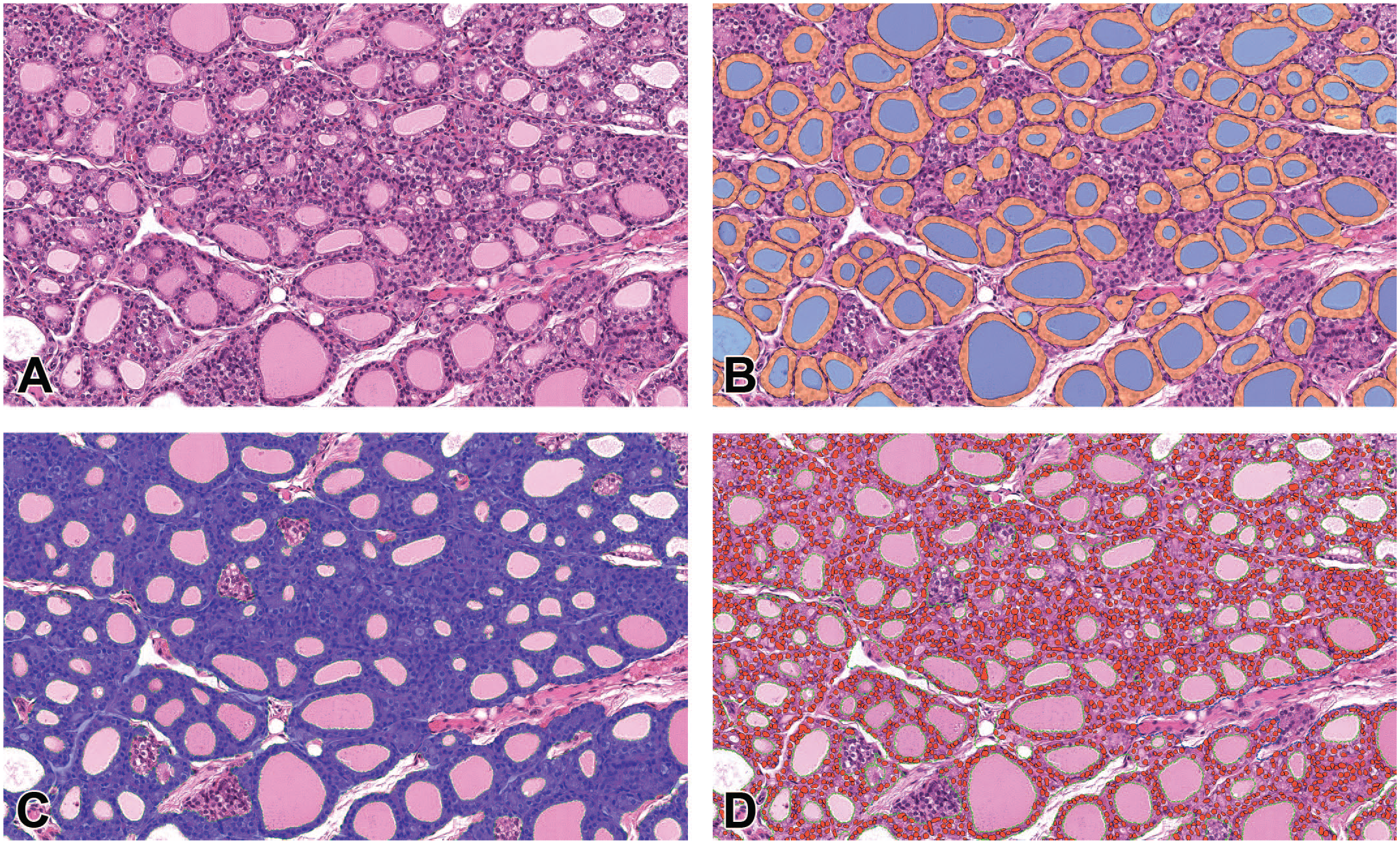
Illustration of segmentation achieved by deep learning IA models 1 and 2. (A) thyroid gland H&E. (B) detection of individual follicles excluding C-cells and incompletely sectioned follicular epithelium. Colloid in blue, intact follicular cell layers in orange. (C) detection of follicular cells and C-Cells in blue. (D) detection of follicular cell and C-cell nuclei in red. Green dashed line colloid ROI.

Figure 2.

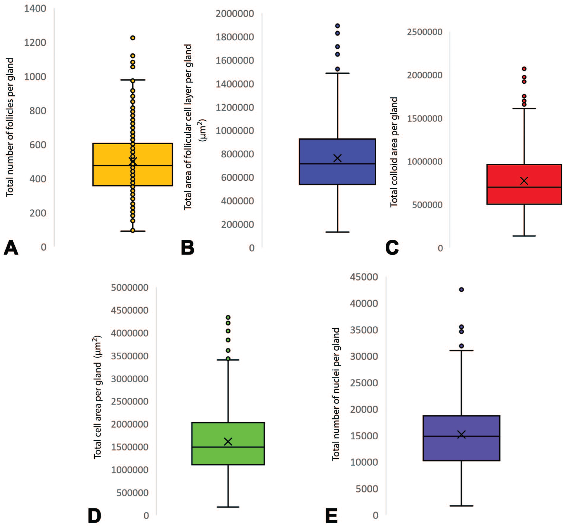
Graphical representation of segmentation achieved by deep learning IA models 1 and 2. (A) Number of follicles identified per section of gland in IA model 1 (x¯ = 500.2, SD = 194.5). (B) Follicular cell layer area, µm², per section of gland in IA model 1 (x¯ = 761,145.7, SD = 318,661.6). (C) Area of colloid, µm², identified per section of gland in IA model 1 (x¯ = 774,233.8, SD = 359,345.4). (D) Total cellular area per gland, µm² in IA model 2 (x¯ = 1,611,725.8, SD = 721,763.4). (E) Total number of nuclei detected per gland in IA model 2 (x¯ = 15,174.6, SD = 6351.1).

Performance of Fixed Calculation Methods and Empirical Models

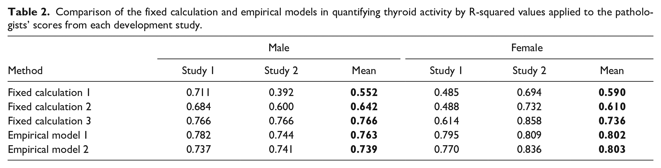
Each empirical model and fixed calculation method was assessed against the pathologists’ scores, generated for the thyroids of males and females from each development study, using the coefficient of determination (R-squared or R²). This value is used to demonstrate the performance of each method by calculating what proportion of variation in the dependent (target) variable (in this case the TAS) is determined by the independent (predictor) variable (pathologists’ scores) in terms of proportion of variance.⁶ As can be seen in Table 2, the mean R² values for the empirical models exceeded 0.7. However, Fixed Calculation Methods 1 and 2 yielded lower mean R² values, in some cases with values below 0.6. Fixed calculation method 3 performed better than the other fixed calculation methods and was comparable to the empirical models in all but one development study (Study 1 female).

Table 2.

Comparison of the fixed calculation and empirical models in quantifying thyroid activity by R-squared values applied to the pathologists’ scores from each development study.

Method	Male			Female
Method	Study 1	Study 2	Mean	Study 1	Study 2	Mean
Fixed calculation 1	0.711	0.392	0.552	0.485	0.694	0.590
Fixed calculation 2	0.684	0.600	0.642	0.488	0.732	0.610
Fixed calculation 3	0.766	0.766	0.766	0.614	0.858	0.736
Empirical model 1	0.782	0.744	0.763	0.795	0.809	0.802
Empirical model 2	0.737	0.741	0.739	0.770	0.836	0.803

Inter-Pathologist Consistency

Inter-pathologist consistency was assessed using a two-way mixed consistency, average-measures intraclass correlation (ICC)¹³ to assess the degree that pathologists provided consistency in their ranking of thyroids across subjects within each development study. An ICC score over 0.75 is considered excellent.⁷ The resulting ICC was in the excellent range, ie, 0.941, 0.918, 0.898, and 0.953, for studies 1M, 2M, 1F, and 2F, respectively, indicating that pathologists had a high degree of agreement in ranking thyroid gland activity. The high ICC suggests that a minimal amount of measurement error was introduced by the independent ranking exercise, and therefore statistical power for subsequent analyses was not substantially reduced. Pathologists’ rankings were therefore deemed to be suitable for use in the testing and development of the various calculations and empirical models.

Selection of Statistical Methods

Many standard statistical tests assume the underlying distribution is normal (Gaussian) and to test this is the case, large control data sets (at least 100 animals) from each sex and study duration (28 and 90 days) were obtained and the various methods applied. For empirical models 1 and 2, normal distribution was demonstrated using the Shapiro-Wilks test,²⁸ although 28-day males and females both required log transformation for empirical model 2. Fixed calculation 3 required log transformation to produce normally distributed data for all control data sets.

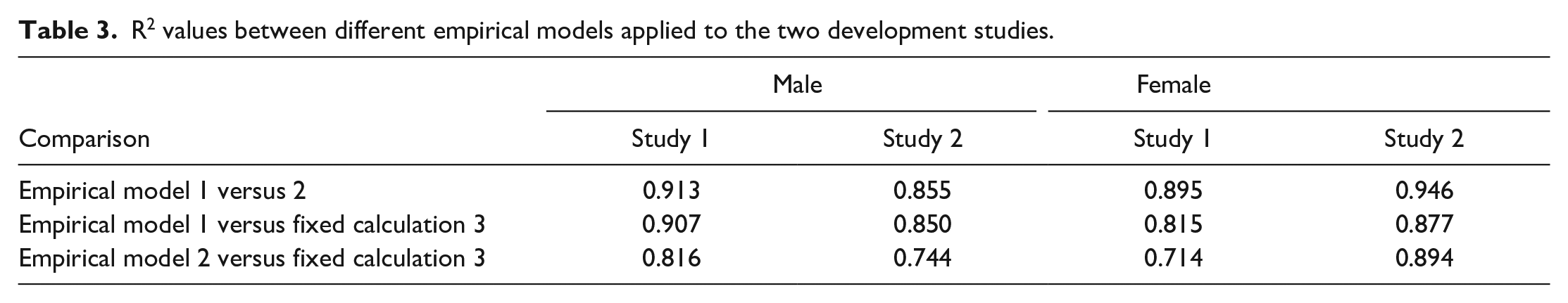
One method commonly employed to analyze continuous normally distributed data across three or more groups is one-way ANOVA.¹⁸ For example, this is typically applied to analysis of organ weight data on safety assessment studies. As three methods were under consideration, rather than selecting just one to take forward, all three could potentially be applied, using appropriate methods to correct for multiple comparisons, eg, Bonferroni.⁵ However, such corrections may reduce statistical power. A method that avoids this restriction and maintains or improves statistical power is the multivariate ANOVA (MANOVA). However, to employ this method several additional assumptions must be assessed, and the relationship between the various approaches, ie, dependent variables, is critical.³² The dependent variables must be moderately correlated, but generally a R² value of greater than 0.8 indicates a risk of multicollinearity, compromising the statistical power. The R² values between the three methods when applied to the development studies (Table 3) and the historical control cohorts (Table 4) are presented. Empirical models 1 versus 2 and Empirical model 1 versus Fixed calculation 3 correlated too closely with one another, with values consistently exceeding 0.8 by a significant margin in both sexes. Empirical model 2 versus Fixed calculation 3 resulted in acceptable R² values for males for most comparisons and therefore the MANOVA would be considered appropriate using these two methods for males. In contrast, Empirical model 2 versus Fixed calculation 3 in females yielded some R² values well above 0.8 and therefore MANOVA would not be used for females.

Table 3.

R² values between different empirical models applied to the two development studies.

Comparison	Male		Female
Comparison	Study 1	Study 2	Study 1	Study 2
Empirical model 1 versus 2	0.913	0.855	0.895	0.946
Empirical model 1 versus fixed calculation 3	0.907	0.850	0.815	0.877
Empirical model 2 versus fixed calculation 3	0.816	0.744	0.714	0.894

Table 4.

R² values between different methods applied to historical control datasets from 28-day and 90-day studies.

Comparison	Male		Female
Comparison	28 Day¹	90 Day	28 Day²	90 Day
Empirical model 1 versus 2	0.873	0.892	0.904	0.901
Empirical model 1 versus fixed calculation 3	0.811	0.826	0.842	0.900
Empirical model 2 versus fixed calculation 3	0.774	0.768	0.806	0.880

1,2

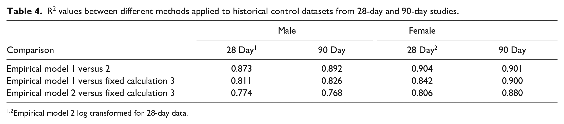
Empirical model 2 log transformed for 28-day data.

Illustration of Empirical Models 1 and 2 for Low and High Scoring Thyroids

As a graphical illustration of how the two empirical models yield TAS values that emphasize differences between thyroids assigned low and high scores by pathologists, various scatter plots are presented in Figures 3 and 4. Each plot represents a single animal, and an example of a low and high scoring individual (based on pathologists’ scores and the TAS) are compared in each of the figures. Each data point represents a single follicle and is assigned a color based on the weighting value applied in that section of the plot. For model 1, each color category represents a single weighting value as used in the actual model, whereas for model 2, the range of values represented by each color has been selected purely for this illustration. The differing approaches to graphical illustration are the result of the way each model works, with model 1 assigning follicles into discrete categories and model 2 treating the measured outputs as continuous data to calculate the TAS.

Figure 3.

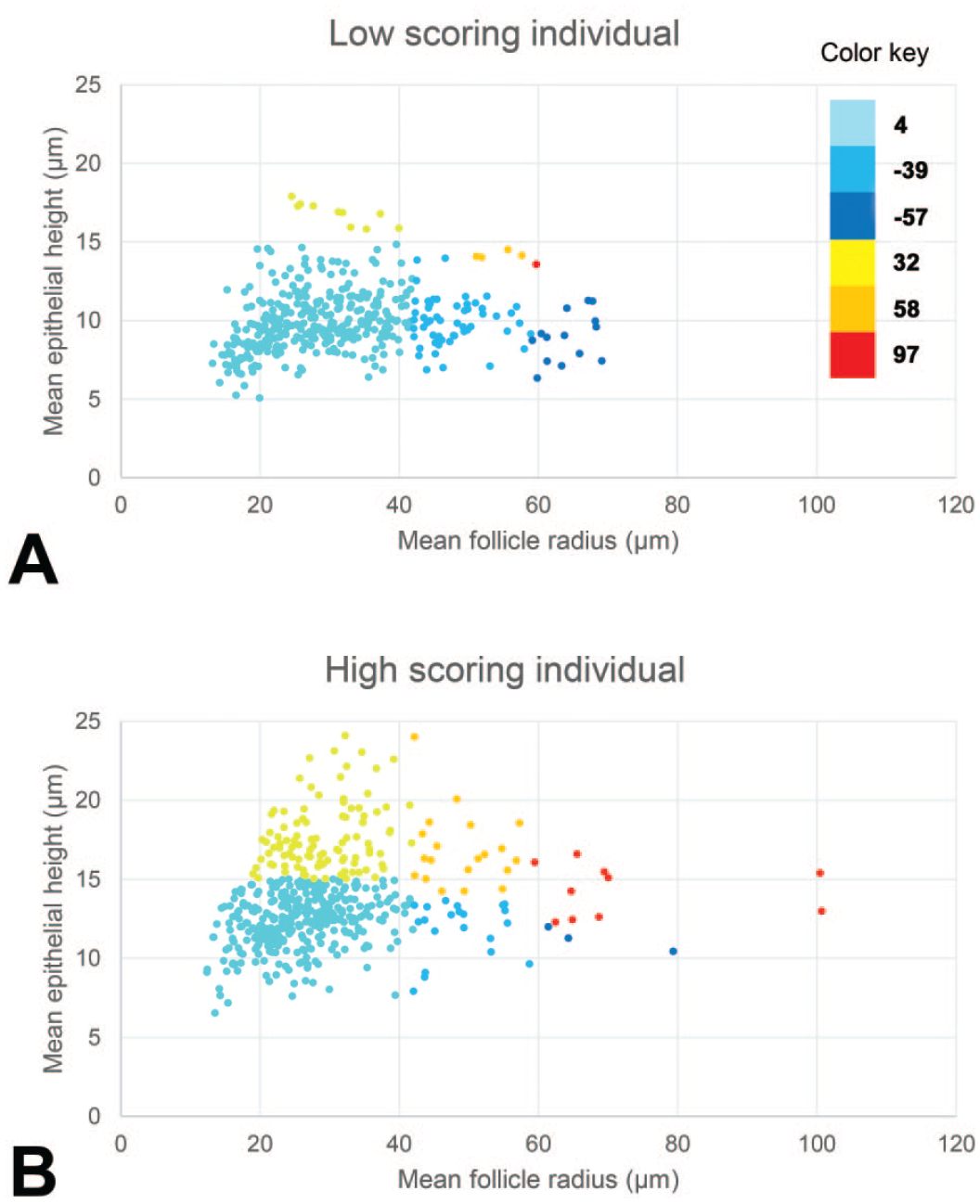
Graphical representation of the individual follicle scores of one animal with a low (A) and one animal with a high (B) scoring thyroid gland produced by empirical method 1. Color-coding is used to indicate the weighting used for each of the segments based on the follicle height and radius. For example, dark blue represents follicles with a low weighting score (−57), while red represents follicles with a high weighting score (97).

Figure 4.

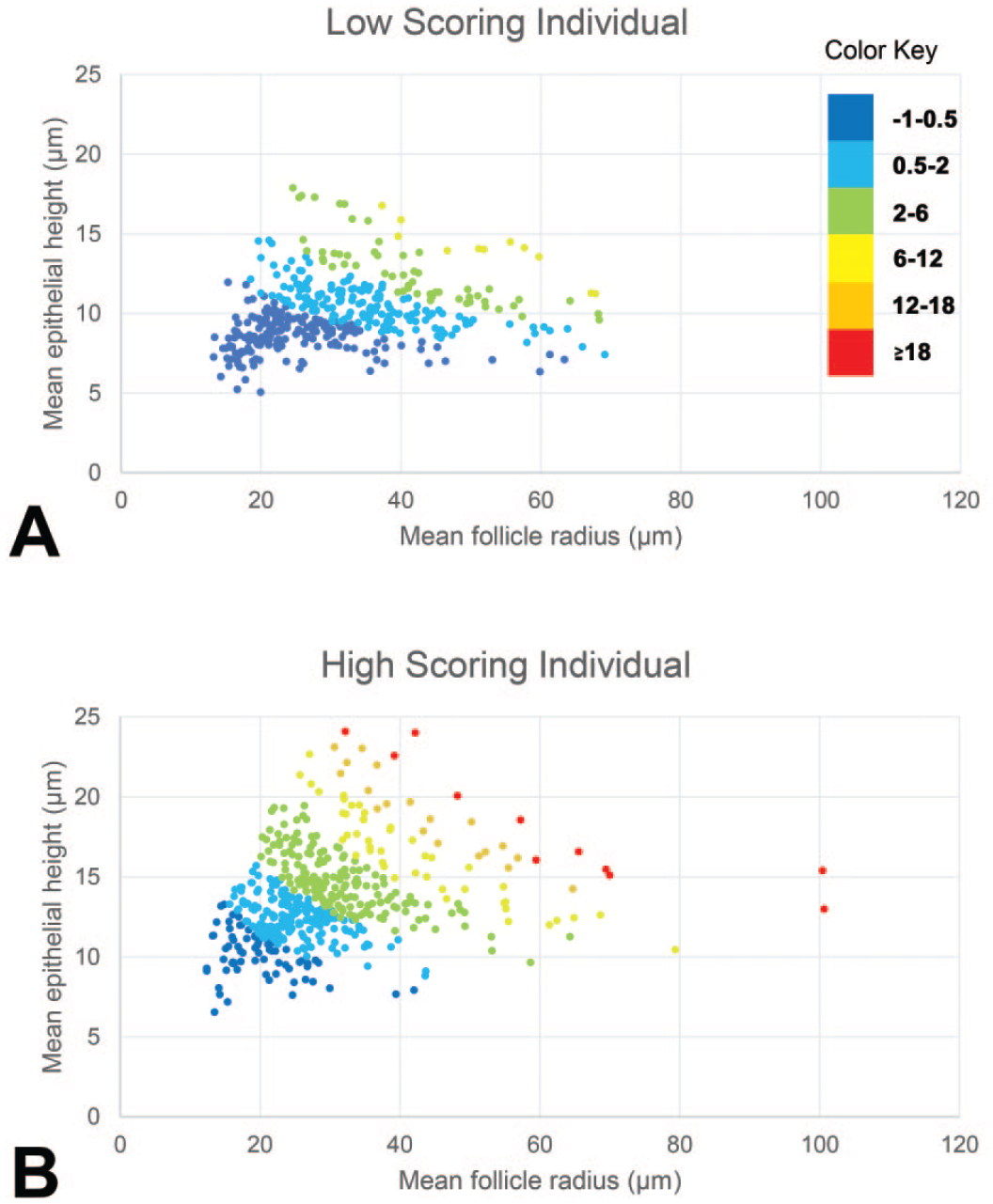
Graphical representation of the individual follicle scores of one animal with a low (A) and one animal with a high (B) scoring thyroid gland produced by empirical method 2. Color-coding for arbitrary ranges of scores based on the follicle height and radius, to highlight the differences. For example, dark blue represents follicles with scores within the range −1 to +0.5, orange represents follicles with scores within the range +12 to +18.

Discussion

The application of deep learning and artificial intelligence to toxicologic pathology has resulted in algorithms promising to provide greater accuracy in the identification of specific histopathological findings.³⁰ Previous workers have applied artificial intelligence to findings in organs such as the kidney,¹⁶ brain,²³ bone marrow,¹⁷ and liver.²⁵

Several image analysis solutions have been proposed to detect thyroid gland hypertrophy. The mean follicular epithelial cell area (MEA) approaches described by Garrido et al,¹⁰ Zabka et al,³⁴ and Bertani et al,² involve detection of total epithelium (excluding colloid and stroma), but include partially transected follicles, neuro-epithelial C-cell populations, and other interstitial cells. By including non-follicular cell populations and partially transected follicles with obliquely sectioned epithelial cells, there is a risk of introducing irrelevant data, diluting real effects with resultant loss of sensitivity and specificity in detecting thyroid hypertrophy. We replicated this approach in IA model 2 (fixed calculation method 2) to allow comparisons to be made to previous published models. Our IA model 1 segments only follicular epithelium associated with defined follicle structures with a complete follicular cell layer and a colloid core, thus eliminating C-cells and obliquely sectioned epithelial layers, to result in an improved version of the mean follicular cell area approach.

An alternative approach demonstrated by Bertani et al² was the hypertrophy area fraction (HAF), using a deep learning algorithm trained to directly detect hypertrophic follicular epithelium in H&E-stained sections and express this as a fraction of the overall follicle gland area. The results generated by such an approach are dictated by the threshold between presence and absence of hypertrophy selected by the pathologists generating the ground-truth annotations. The limitations of the MEA and HAF approaches are illustrated in the Bertani paper by their ability to distinguish between different grades of hypertrophy. With a direct thyroid toxicant when higher grades were included in the analysis there was good correlation between the pathologist’s grades and the MEA and HAF scores (Spearman r values of 0.75-0.85 and 0.81, respectively). However, with a liver-mediated thyroid toxicant inducing only minimal and mild grades, with considerable overlap between the negative and minimal, and minimal and mild grades, with respect to the MEA and HAF scores, there was relatively poor correlation (0.57 and 0.61, respectively).

We therefore developed methods specifically to assist in the detection of low-grade microscopic thyroid follicular cell hypertrophy with the premise that grades of mild or above are only considered if there are obvious and unequivocal morphological changes readily detected by pathologists. Improving consistency in delineating different grades, is only one benefit of an IA pathology solution. An arguably more practically useful outcome is the establishment of the NOEL (no observable effect level) and at the lowest dose level affected in a study, grades higher than minimal are unusual. As there is considerable variation in the activity and resulting appearance of control rat thyroids that often include some examples pathologists may consider to be low-grade hypertrophy, our approach was to develop an IA solution to quantify the variation present within control rats as well as those with borderline and low-grade hypertrophy. Once this variation is captured numerically, effects at the group level can be assessed statistically to determine the NOEL, leaving the pathologist to make the ultimate decision of which animals to record hypertrophy in.

Essential to this approach was the capture of the range of appearances seen in control, borderline hypertrophic and low-grade hypertrophic thyroids. To achieve this, pathologists were asked to subjectively rank batches of thyroids in terms of this spectrum of appearance. Inevitably there was a degree of disagreement between individual pathologists on specific animals and batches, but by averaging the ranked values, extreme differences of opinion canceled out and a consensus score representing a ground-truth equivalent was produced. The degree of inter-pathologist consistency was quantified using published methods and the ICC was demonstrated as excellent for all the development studies.

The MEA approach does not take into account variation between individual follicles and just presents an overall mean value. Bertani et al² demonstrated that the colloid area fraction is inversely proportional to MEA which increased with hypertrophy grade. As an alternative fixed calculation method, we therefore calculated the mean follicle epithelial area: colloid area ratio, with an adjustment to allow for the overall area fraction of each individual follicle. To further exploit information at the individual follicle level, we used empirical models. These models selected optimal values of various parameters within each model architecture that emphasized or suppressed the impact of individual follicles to align with the pathologists’ scores.

Fixed calculation methods 1 and 2 applied to the various development batches of thyroids yielded broadly similar R² values, with method 2 (our version of MEA) slightly better than model 1 (mean follicle epithelial area: colloid area ratio). Fixed calculation method 3 and the two empirical models were selected as potential methods to take forward as they yielded R² values consistently higher than the first two fixed calculations, and critically did so with two independent batches of thyroids, although Fixed calculation 3 underperformed slightly with one of the female development studies. What constitutes an acceptable R² value depends on the type of data that are being modeled. In social sciences, modeling complex human behavior, 0.1 or above may be acceptable, but in physical sciences, involving processes generally more predictable than those encountered in life or social sciences (eg, modeling the behavior of atoms or molecules), a value below 0.6 is considered weak and values of greater than 0.7 are generally considered acceptable.^22,24,31 Both empirical models produced R² values higher than 0.7, in many cases substantially higher. It should be noted that for comparison to the Pearson R² values reported in this article, the Spearman r values stated by Bertani et al² and quoted above should be converted to r² values, ie, the MEA and HAF r² values for the liver-mediated thyroid toxicant would be 0.32 and 0.38, respectively. However, it is considered likely that much of the difference between these values and those reported in this article are due to the different methods of generating pathologists’ grades/scores, rather than the performance of the algorithms.

The approach adopted in this article identified three similarly performing methods to quantify thyroid gland activity and provide a means by which test article effects at the group level can be assessed. It is desirable to have data that are normally distributed as this justifies the use of parametric statistical tests such as ANOVA. These are considered the optimal approaches for analysis of continuous data in multiple treatment groups and frequently employed in toxicity studies to assess endpoints such as organ weights. Rather than assume our methods result in data with a normal, or Gaussian, distribution, cohorts of control animals of both sexes from studies of the durations used in sub-chronic toxicity studies in rodents (28 and 90 days), with at least 100 animals of each category, were tested for normality using the Shapiro-Wilk test.²⁸ All were normally distributed, although in some instances log transformation was required.

Rather than selecting just one method to take forward, there may be advantages in using multiple methods, such as avoiding over-reliance on any one method, but applying multiple statistical tests requires an adjustment to the level of significance, offsetting some of the advantage. To avoid this limitation, the statistical approach of MANOVA was considered. Certain criteria must be met for this statistical approach, and most must be assessed on a study specific basis. However, it is critical to avoid multicollinearity, a consequence of excessive correlation between methods. Therefore, the correlations between the three methods were determined using historical control cohorts of at least 100 animals for each sex and study duration. Based on this, empirical model 2 and fixed calculation method 3 could be used collectively for the MANOVA in males, but other combinations correlated too highly. This can be viewed positively, in that strong agreement between different methods when assessed in this manner provides a form of mutual validation.

Other methods to quantify thyroid hypertrophy may be available, for example, the hypertrophy area fraction approach described by Bertani et al.² The use of statistical approaches that encompass multiple methods allows for the integration of additional approaches into the analysis, provided of course, they meet the requirements described above, ie, correlation with pathologists’ scores, normal distribution, and appropriate correlations between methods.

Another statistical approach could be to compare each group on a study, including the control group, to a large set of historic controls from the same study type/duration. This would provide a better representation of the distribution within the control population and avoid the risk of outliers in a study control group skewing the results. This is not possible for ANOVA due to the requirement to compare groups of the same or similar size. Methods that are insensitive to group size would have to be applied, such as Welch’s t-test.³³

In conclusion, this study has generated algorithms and subsequent processing steps that can be applied to whole slide images of thyroid gland sections from toxicity studies in rats to yield quantifiable outputs that correlate highly with pathologists’ scores. The use of appropriate statistical methods to assess the presence or absence of low-grade thyroid hypertrophy at the group level and integration of this process into a safety assessment workflow to support the study pathologist’s decision process will be relatively straight forward to implement.

Supplemental Material

sj-docx-1-tpx-10.1177_01926233241309328 – Supplemental material for Development of a Deep Learning Tool to Support the Assessment of Thyroid Follicular Cell Hypertrophy in the Rat

Supplemental material, sj-docx-1-tpx-10.1177_01926233241309328 for Development of a Deep Learning Tool to Support the Assessment of Thyroid Follicular Cell Hypertrophy in the Rat by Stuart W. Naylor, Elizabeth F. McInnes, James Alibhai, Scott Burgess and James Baily in Toxicologic Pathology

Supplemental Material

sj-docx-2-tpx-10.1177_01926233241309328 – Supplemental material for Development of a Deep Learning Tool to Support the Assessment of Thyroid Follicular Cell Hypertrophy in the Rat

Supplemental material, sj-docx-2-tpx-10.1177_01926233241309328 for Development of a Deep Learning Tool to Support the Assessment of Thyroid Follicular Cell Hypertrophy in the Rat by Stuart W. Naylor, Elizabeth F. McInnes, James Alibhai, Scott Burgess and James Baily in Toxicologic Pathology

Supplemental Material

sj-docx-3-tpx-10.1177_01926233241309328 – Supplemental material for Development of a Deep Learning Tool to Support the Assessment of Thyroid Follicular Cell Hypertrophy in the Rat

Supplemental material, sj-docx-3-tpx-10.1177_01926233241309328 for Development of a Deep Learning Tool to Support the Assessment of Thyroid Follicular Cell Hypertrophy in the Rat by Stuart W. Naylor, Elizabeth F. McInnes, James Alibhai, Scott Burgess and James Baily in Toxicologic Pathology

Supplemental Material

sj-docx-4-tpx-10.1177_01926233241309328 – Supplemental material for Development of a Deep Learning Tool to Support the Assessment of Thyroid Follicular Cell Hypertrophy in the Rat

Supplemental material, sj-docx-4-tpx-10.1177_01926233241309328 for Development of a Deep Learning Tool to Support the Assessment of Thyroid Follicular Cell Hypertrophy in the Rat by Stuart W. Naylor, Elizabeth F. McInnes, James Alibhai, Scott Burgess and James Baily in Toxicologic Pathology

Footnotes

Acknowledgements

The authors thank Agnieszka Gorczyca for her technical expertise with Visiopharm software to generate the IA models. The authors thank the digital pathology technicians, Nyree Cowe and Heather Watts of Charles River Laboratories, Edinburgh, for the retrieval and digitalization of glass slides, and Petrina Rogerson and Begonya Garcia of Charles River Laboratories, Edinburgh and Evreux, for contributing to the histopathology scoring.

Declaration of Conflicting Interests

The author(s) declared the following potential conflicts of interest with respect to the research, authorship, and/or publication of this article: Stuart Naylor, James Alibhai and James Baily are currently employed by Charles River Laboratories Ltd., a contract research organization. Elizabeth McInnes is currently an employee of Syngenta Ltd., a developer of agricultural products. None of the authors received a compensation, in addition to their salary, for this publication. This research study was a method development study. Results are published to make concepts and data available for the public and do not promote a product commercially exploited by Syngenta Ltd. Some or all the methods described may in future be implemented as a commercially available product to assist with pathology decision-making on safety assessment studies conducted at Charles River Laboratories Ltd.

Funding

The author(s) disclosed receipt of the following financial support for the research, authorship, and/or publication of this article: This work was funded by a Syngenta Product Safety Strategic Science grant.

ORCID iD

Stuart W. Naylor

Supplemental Material

Supplemental material for this article is available online.

References

Bars

Broeckaert

Fegert

, et al. Science based guidance for the assessment of endocrine disrupting properties of chemicals. Regul Toxicol Pharmacol. 2011;59(1):37-46.

Bertani

Blanck

Guignard

Schorsch

Pischon

. Artificial intelligence in toxicological pathology: quantitative evaluation of compound-induced follicular cell hypertrophy in rat thyroid gland using deep learning models. Toxicol Pathol. 2022;50(1):23-34.

Bolon

Caverly Rae

Colman

, et al. Opinion on current use of non-blinded versus blinded histopathologic evaluation in animal toxicity studies. Toxicol Pathol. 2020;48(4):549-559.

Brändli-Baiocco

Balme

Bruder

, et al. Nonproliferative and proliferative lesions of the rat and mouse endocrine system. J Toxicol Pathol. 2018;31(3):1S-95S.

Chen

Feng

. A general introduction to adjustment for multiple comparisons. J Thorac Dis. 2017;9(6):1725-1729.

Chicco

Warrens

Jurman

. The coefficient of determination R-squared is more informative than SMAPE, MAE, MAPE, MSE and RMSE in regression analysis evaluation. Peerj Computer Science. 2021;7:e623. https://doi.org/10.7717/peerj-cs.623

Cicchetti

. Guidelines, criteria, and rules of thumb for evaluating normed and standardized assessment instrument in psychology. Psychol Assess. 1994;6(4):284-290.

Fisher

Campbell

Muralidhara

, et al. Effect of PCB 126 on hepatic metabolism of thyroxine and perturbations in the hypothalamic-pituitary-thyroid axis in the rat. Toxicol Sci. 2006;90(1):87-95.

Foster

Tinwell

Melching-Kollmuss

. A review of species differences in the control of, and response to, chemical-induced thyroid hormone perturbations leading to thyroid cancer. Arch Toxicol. 2021;95(3):807-836.

10.

Garrido

Zabka

Tao

Fielden

Fretland

Albassam

. Quantitative histological assessment of xenobiotic-induced liver enzyme induction and pituitary-thyroid axis stimulation in rats using whole-slide automated image analysis. J Histochem Cytochem. 2013;61(5):362-371.

11.

Ghassabian

Trasande

. Disruption in thyroid signaling pathway: a mechanism for the effect of endocrine-disrupting chemicals on child neurodevelopment. Front Endocrinol (Lausanne). 2018;9:article204.

12.

Giles

Romano

Markkula

. Bayesian analysis of subjective ranking data using Thurstonian models: tutorial, novel methods, and an open-source library. Published 2018. Accessed December 13, 2024. https://osf.io/preprints/psyarxiv/t7szv

13.

Hallgren

. Computing inter-rater reliability for observational data: an overview and tutorial. Tutor Quant Methods Psychol. 2012;8(1):23-34.

14.

Huisinga

Bertrand

Chamanza

, et al. Adversity considerations for thyroid follicular cell hypertrophy and hyperplasia in nonclinical toxicity studies: results from the 6th ESTP international expert workshop. Toxicol Pathol. 2020;48(8):920-938.

15.

Jugan

Levi

Blondeau

. Endocrine disruptors and thyroid hormone physiology. Biochem Pharmacol. 2010;79(7):939-947.

16.

Kolachalama

Singh

Lin

, et al. Association of pathological fibrosis with renal survival using deep neural networks. Kidney Int Rep. 2018;3(2):464-475.

17.

Kozlowski

Brumm

Cain

. An automated image analysis method to quantify veterinary bone marrow cellularity on H&E sections. Toxicol Pathol. 2018;46(3):324-335.

18.

Larson

. Analysis of variance. Circulation. 2008;117(1):115-121.

19.

Laurberg

Bournaud

Karmisholt

Orgiazzi

. Management of Graves’ hyperthyroidism in pregnancy: focus on both maternal and foetal thyroid function, and caution against surgical thyroidectomy in pregnancy. Euro J Endocrinol. 2009;160:1-8.

20.

Ledder

. Empirical Modelling. In: Mathematical Modeling for Epidemiology and Ecology. 2nd ed. Cham, Switzerland: Springer Nature; 2023. doi:10.1007/978-3-031-09454-5_2.

21.

Maki

. Inter-rater reliability in healthcare studies: calculating the intraclass coefficient (ICC) in SAS. SAS Institute. Accessed July 30, 2024. https://www.sas.com/content/dam/SAS/en_ca/User%20Group%20Presentations/Health-User-Groups/Maki-InterraterReliability-Apr2014.pdf

22.

Paul

. How to check for a good regression model by R-squared? Accessed April 10, 2024. https://sspaulc.medium.com/how-to-check-for-a-good-regression-model-by-r-squared-7878dc3ff3c5

23.

Penttinen

Parkkinen

Blom

, et al. Implementation of deep neural networks to count dopamine neurons in substantia nigra. Eur J Neurosci. 2018;48(6):2354-2361.

24.

Peterson

. Munich personal RePEc archive. The acceptable R-square in empirical modelling for social science research. Published 2023. Accessed April 10, 2024. https://mpra.ub.uni-muenchen.de/116496/

25.

Pischon

Mason

Lawrenz

, et al. Artificial intelligence in toxicologic pathology: quantitative evaluation of compound-induced hepatocellular hypertrophy in rats. Toxicol Pathol. 2021;49(4):928-937.

26.

Roberts

. A formula for the perimeter of an ellipse. Accessed April 10, 2024. https://extremelearning.com.au/a-formula-for-the-perimeter-of-an-ellipse/

27.

SAS Institute Inc. SAS/STAT software, Version 9.4M5 of the SAS System for Windows. Copyright © 2017 SAS Institute Inc. SAS and all other SAS Institute Inc. product or service names are registered trademarks or trademarks of SAS Institute Inc., Cary, NC, USA. www.sas.com

28.

Shapiro

Wilk

. An analysis of variance test for normality (complete samples). Biometrika. 1965;52:591-611.

29.

Thambirajah

Wade

Verreault

, et al. Disruption by stealth—Interference of endocrine disrupting chemicals on hormonal crosstalk with thyroid axis function in humans and other animals. Environ Res. 2022;203:111906.

30.

Turner

Aeffner

Bangari

, et al. Opinion on the application of artificial intelligence and machine learning to digital toxicologic pathology. Toxicol Pathol. 2019;48(2):277-294.

31.

Valchanov

. Measuring explanatory power with the R-squared. 365 DataScience. Accessed April 10, 2024. https://365datascience.com/tutorials/statistics-tutorials/r-squared/

32.

Warner

. A primer on multivariate analysis of variance (MANOVA) for behavioral scientists. Pract Assess Res Eval. 2014;19(1):Article17.

33.

Wikipedia. Welch’s t-test. Accessed July 30, 2024. https://en.wikipedia.org/wiki/Welch%27s_t-test

34.

Zabka

Fielden

Garrido

, et al. Characterization of xenobiotic induced hepatocellular enzyme induction in rats: anticipated thyroid effects and unique pituitary gland findings. Toxicol Pathol. 2011;39(4):664-677.

Supplementary Material

Please find the following supplemental material available below.

For Open Access articles published under a Creative Commons License, all supplemental material carries the same license as the article it is associated with.

For non-Open Access articles published, all supplemental material carries a non-exclusive license, and permission requests for re-use of supplemental material or any part of supplemental material shall be sent directly to the copyright owner as specified in the copyright notice associated with the article.

0.00 MB

0.02 MB

0.01 MB