
Abstract
In preclinical toxicology studies, a “stage-aware” histopathological evaluation of testes is recognized as the most sensitive method to detect effects on spermatogenesis. A stage-aware evaluation requires the pathologist to be able to identify the different stages of the spermatogenic cycle. Classically, this evaluation has been performed using periodic acid-Schiff (PAS)-stained sections to visualize the morphology of the developing spermatid acrosome, but due to the complexity of the rat spermatogenic cycle and the subtlety of the criteria used to distinguish between the 14 stages of the cycle, staging of tubules is not only time consuming but also requires specialized training and practice to become competent. Using different criteria, based largely on the shape and movement of the elongating spermatids within the tubule and pooling some of the stages, it is possible to stage tubules using routine hematoxylin and eosin (H&E)-stained sections, thereby negating the need for a special PAS stain. These criteria have been used to develop an automated method to identify the stages of the rat spermatogenic cycle in digital images of H&E-stained Wistar rat testes. The algorithm identifies the spermatogenic stage of each tubule, thereby allowing the pathologist to quickly evaluate the testis in a stage-aware manner and rapidly calculate the stage frequencies.
Introduction
Examination of rodent testes with an awareness of staging has been a regulatory recommendation for certain types of preclinical toxicity studies for many years. 1 Generally, this has been performed on specially prepared periodic acid-Schiff (PAS) stained sections by a pathologist who has received training on how to stage testes. The reason for using PAS-stained testes is so that the details of the developing acrosome of the round spermatid (RSp) can be visualized and used to distinguish between the first 8 stages (stages I-VIII) of the 14 stages of the spermatogenic cycle of the rat. The final 6 stages of the spermatogenic cycle (stages IX-XIV) are identified using the changing shape of the elongating spermatid head. Although not the only classification system for rodent spermatogenesis, this 14-stage scheme, described by Leblond and Clermont in 1952, 2 has become the most commonly used method to stage rodent testes. While it is a very good and accurate method to stage rodent testes, it is not very practical for inclusion in routine histopathological assessment, partly because of technical difficulties in getting the PAS to stain the acrosomic structures adequately but also because distinguishing between the 14 stages of the spermatogenic cycle is difficult and requires significant training and expertise. One of the main reasons for staging tubules during histopathological assessment of spermatogenesis is to allow the pathologist to identify subtle disturbances in spermatogenesis and recognize when a cell population that should be present is missing, or when a cell population is inappropriately present. 3 However, this “stage-awareness” does not require such detailed staging as the Leblond and Clermont 2 scheme affords. Identification of these subtle changes can be achieved, as long as the pathologist is familiar with the overall cell composition of tubules in the main phases of the cycle, that is, early (stages I-VI), mid (stages VII-VIII), and late (stages IX-XIV) stages of the spermatogenic cycle. This level of stage recognition can be accomplished relatively easily using hematoxylin and eosin (H&E) staining. 4 An important advantage of performing staging on H&E-stained testes is that these sections are routinely available for most toxicity studies and negate the need to perform special PAS staining. The detailed criteria used for staging H&E-stained rat testes have been described previously by Creasy and Chapin. 4 They utilize the changing shape and position of the elongated spermatid in the early stages (stages I-VI), the size and position of the residual body (RB) for mid stages (VII-VIII), and the shape and morphology of the elongating spermatid to identify the late stages (IX-XIII), plus the presence of meiotic spermatocytes (Spcs) for stage XIV. 4 Although this H&E-based methodology is not as accurate as using the PAS-based characteristics of the acrosome, it is easier to adapt to automated digital technology and it provides sufficient stage recognition to allow the pathologist to conduct a detailed, stage-aware evaluation on toxicity screening studies up to 28 days duration (as recommended in the Society of Toxicologic Pathology [STP] Position Paper on Evaluation of Testes). 1 If any stage-specific abnormalities are detected in these short-term screening studies, then it may be necessary to perform additional PAS-stained sections to study them in more detail.
To aid the pathologist in the staging of H&E-stained rat testes, we have developed an algorithm that uses these and other criteria to annotate individual tubules in digital scans of testis sections. The staging algorithm was developed by using deep learning 5,6 and machine learning-based methods. 7,8 Training of the software was performed by comparing the staging results of the algorithm with the staging results of an expert pathologist (DC) on a subset of H&E-stained testis images. Annotations on individual tubules were generated by the algorithm and were then checked and confirmed or corrected by the pathologist. Progressive improvements on the algorithm criteria were introduced until an acceptable degree of accuracy and precision were achieved between the staging results of the algorithm and the pathologist. Accuracy and precision were assessed using the stage frequency distribution of the results. The algorithm was then validated on a further subset of images by the same pathologist, who reviewed each algorithm-generated annotation and either confirmed or corrected the annotation. In addition, stage frequency maps were generated for the algorithm-generated staging data and for the pathologist-generated staging data and were compared with the stage frequency maps for PAS-stained testes that have been published by Hess et al. 9 This validated algorithm identifies the spermatogenic stage of each tubule, thereby allowing the pathologist to quickly evaluate the H&E-stained testis in a stage-aware manner and rapidly calculate stage frequencies.
Materials and Methods
Animal Source and Testes Fixation
The testes used in the development of the staging algorithm came from Wistar rats from a study conducted to collect in-life and pathology data from untreated Wistar rats at different ages (50 males/age-group). The study was performed at WuXi AppTec (Suzhou) Co, Ltd. The Wistar rats were obtained from BioLASCO Taiwan Co, Ltd and acclimated to standard laboratory conditions for a week before study start. The rats that were used to provide testis sections for the development of the staging algorithm were 11 to 15 weeks of age at necropsy. They were euthanized with isoflurane and observed for gross pathology before tissues were collected.
Testes were fixed in modified Davidson’s fluid for 24 to 72 hours before being transferred to 10% neutral buffered formalin for storage. Testes were trimmed (transversely), processed, and embedded in paraffin blocks; sectioned at 3 to 5 microns, mounted on glass microscope slides, and stained with H&E using standard procedures.
In total, 33 whole slide images (WSIs) of individual testes (transverse section) were used from 33 rats; 20 images were used for algorithm development and 13 images were used for validating the algorithm.
Environmental Conditions and Ethical Use of Animals
The original study that provided the untreated rats was carried out according to the principles stated in the Guide for the Care and Use of Laboratory Animals, National Research Council (2011) and The People’s Republic of China, Ministry of Science & Technology, “Regulations for the Administration of Affairs Concerning Experimental Animals,” 1988. The protocol was approved by the WuXi AppTec Institutional Animal Care and Use Committee, and the test facility is Good Laboratory Practice certified and accredited by Association for Assessment and Accreditation of Laboratory Animal Care International.
The Wistar rats were housed in an individually ventilated cage system using polysulfone cages, sterilized corncob was provided as bedding material, and environment enrichment was provided. Controlled environment was maintained (light: 12-hour light/12-hour dark, temperature: 20 °C-26 °C, relative humidity: 30%-70%). Animals were supplied with rodent feed from Beijing Keao Xieli Feed Co, Ltd and chlorinated, reverse osmosis water, ad libitum.
Generation of Digital Images
Whole slide images of the H&E-stained testis sections were generated using Leica SCN400 & Nanozoomer XR (Hamamatsu) scanners at 40× original magnification. These digital images were read by using the software libraries from OpenSlide software, which is a vendor-neutral software for digital pathology. Using this software, we extracted 512 × 512 × 3 dimension tiles at 2.5×, 10×, and 40× resolutions. The tiles were chosen to segment out various parameters, that is, tubule, lumen, and the different germ cells, namely RSps, elongating/elongated spermatids (ESps), Spcs (pachytene), spermatogonia (Spg), and meiotic figures (MFs). Only transversely sectioned tubules were included in the staging classification, longitudinally sectioned tubules were excluded because they usually include more than one stage of the spermatogenic cycle and generally do not provide an adequate cross section of seminiferous epithelium for evaluation. This exclusion of longitudinally sectioned tubules was performed by the algorithm on the basis of the minor axis of the tubule.
Establishment of Staging Criteria
The 14-stage scheme of Leblond and Clermont 2 for PAS-stained testes was used for classifying the spermatogenic cycle but the staging criteria described by Creasy and Chapin 4 for H&E-stained sections were used as the basis for the establishment of criteria for the algorithm. The tubules were staged using the criteria described in Table 1. These criteria were formulated based on the presence or absence of certain germ cells and RBs, along with their morphological features such as shape, size, and relative position within the seminiferous epithelium. The various germ cells used in the criteria were RSps, ESps, pachytene Spcs, Spg. Also, the presence of RBs and MFs were used. Due to the difficulties in separating out all 14 stages of spermatogenesis in H&E-stained sections (vs PAS-stained sections), we decided to combine some of the stages. In the initial stages of algorithm development, we combined stage II with III and combined stage IV with V, thereby producing 12 stages rather than 14. In the later stages of development, we also combined stage VI with IV and V, and we combined stage XII with stage XIII, thereby producing 10 different staging groups. Our rationale for doing this will be provided in the Discussion section.
Staging Criteria for H&E-Stained Testes.
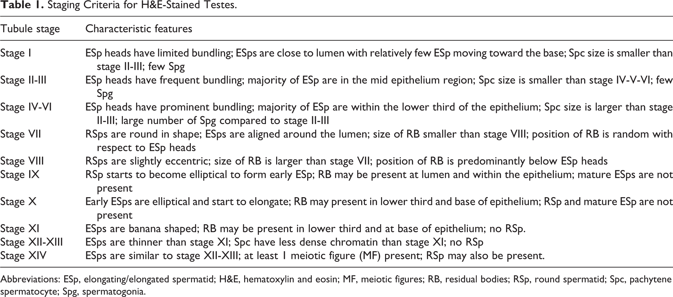
Abbreviations: ESp, elongating/elongated spermatid; H&E, hematoxylin and eosin; MF, meiotic figures; RB, residual bodies; RSp, round spermatid; Spc, pachytene spermatocyte; Spg, spermatogonia.
Data Sets
Tiles from 33 WSIs were used for the development of this algorithm. The WSIs were divided into 2 mutually exclusive data sets, namely a development data set and a validation data set comprising tiles from 20 and 13 WSIs, respectively. The staging algorithm was developed and trained using the development data set and validated on the validation data set. The development and training of the algorithm involved 2 tasks: (1) semantic segmentation of the tubules, lumen, and various germ cells; and (2) classification of the tubules into respective stage groups. For the semantic segmentation task, the development data set was further divided into 2 subsets namely a training data set and a test data set comprising tiles from 15 and 5 WSIs, respectively. Not all the tiles from the corresponding WSIs were used for creating the training and test data sets but were hand-picked, choosing most of the tiles from the tissue region and only 2% to 3% of the tiles from the nontissue region. The groundtruth marking on the selected tiles was performed by in-house data marking experts under the guidance of expert pathologists. The U-Net-based deep learning models were trained using the tiles from the training data set and the test data set. The trained models were then tested on the tiles from the validation data set WSIs. Similarly, for the classification task, the development data set was divided into 2 subsets namely a training data set and a test data set comprising tubules from 15 and 5 WSIs, respectively. The decision tree classifier was trained on these tubules. The trained decision tree classifier was then used to stage tubules in the validation data set WSIs and these staging results were then verified or corrected by the expert pathologist. The makeup of the data sets, the workflow, and the output of the entire process are summarized in Figure 1 and discussed in more detail subsequently.
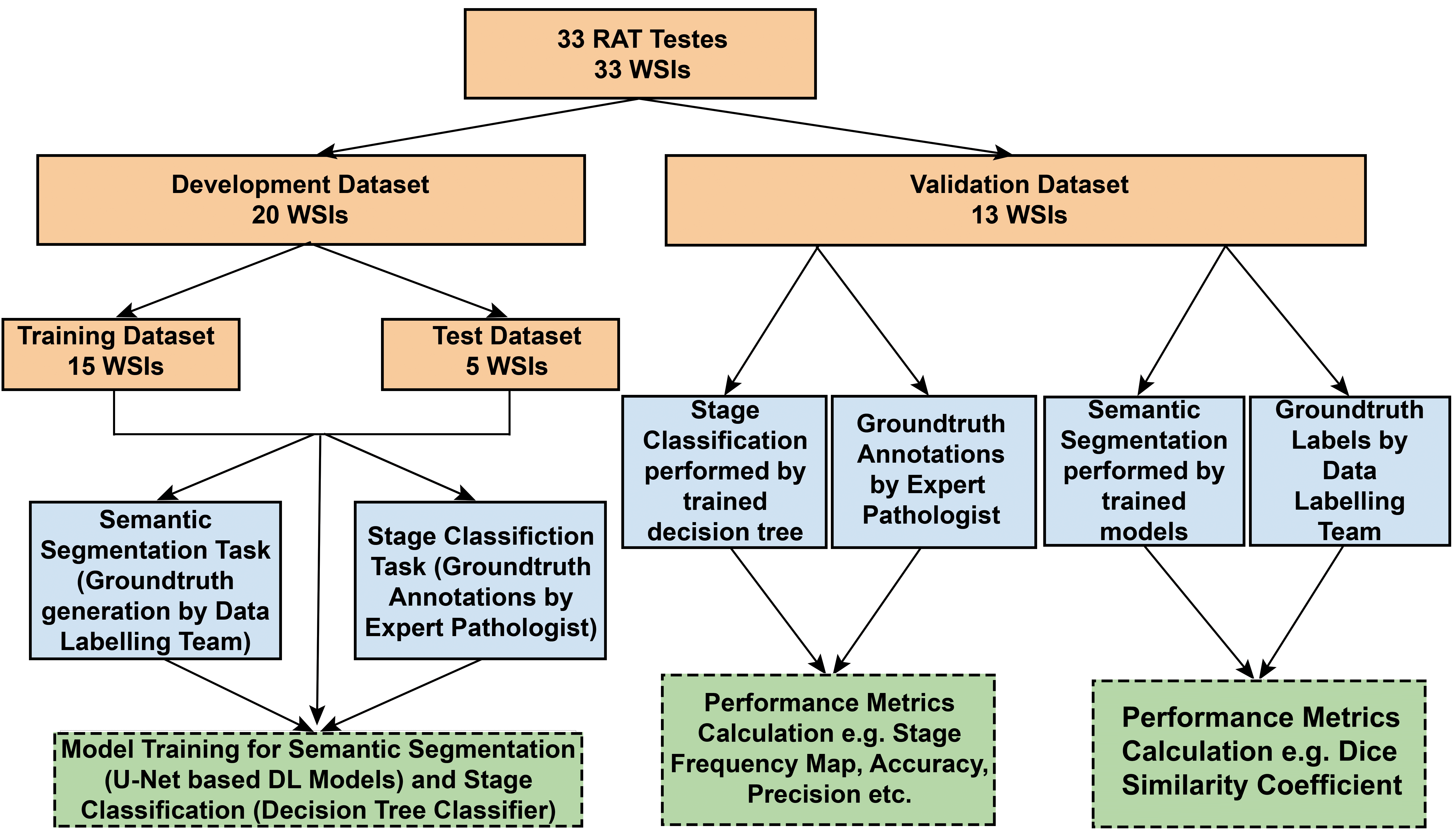
Data sets and flow diagram illustrating the overall development, training, and validation of the staging algorithm. Data sets are highlighted in orange, workflow tasks in blue, and output from the tasks in green. WSI = whole slide image.
Development, Training, and Validation of the Algorithm: Overview of Entire Process
The algorithm was developed through close cooperation between the algorithm development team and a pathologist, expert in staging testes (DC). Initially, a small number of WSIs from the development data set of images were staged by the pathologist and each tubule was annotated with the appropriate stage number. The annotated images were then reviewed with the algorithm development expert (RG), and the main features used for staging were discussed as well as the difficulties associated with delineating where one stage ends and the next begins. Based on these discussions, the algorithm development team produced a preliminary algorithm using the presence of RSps and Spcs, shape, and position of elongating spermatid heads within the tubular epithelium, presence of RBs along with their size, and presence of MFs. This algorithm was used to annotate all the tubules in the 15 WSIs from the training data set of images. The pathologist then reviewed the same tubules and provided a separate annotation. At the end of this exercise, each tubule had 2 annotations, 1 produced by the algorithm and 1 produced by the pathologist.
The tubular staging results of the algorithm were compared with those of the pathologist and any major discrepancies for particular stages were noted. In addition, the consistency of the staging results was tested, by calculating the frequency distribution of stages for each WSI. This was calculated for the algorithm results and the pathologist’s results individually. The frequency of each stage of the spermatogenic cycle is relatively consistent between individual rats, and the frequency distribution of stages in PAS-stained Sprague-Dawley testes has been published by Hess et al. 9 We compared the frequency distribution of stages classified by the pathologist and by the algorithm within a data set of H&E-stained testes against the frequency distribution published by Hess et al 9 in PAS-stained testes to provide a gauge of consistency and accuracy. Following identification of the main discrepancies between the staging results of the algorithm and the pathologist, it was decided to add additional criteria to the algorithm to improve its accuracy. These included taking into account the relative numbers of Spg and the relative size of pachytene Spcs in each tubule. In addition, the position of the RBs with respect to the elongating spermatid head at the tubular lumen was added as an additional criterion for stages VII and VIII. Due to the difficulties of separating stages XII and XIII and stages V and VI consistently (both by the pathologist and the algorithm), it was decided to pool these stages. So, the final 10 pools of stages consisted of stages I, II-III, IV-VI, VII, VIII, IX, X, XI, XII-XIII, and XIV. This new algorithm was then used to annotate the 5 WSIs in the test data set of images and compared with the annotations provided by the pathologist on the same data set.
This improved algorithm was then tested on the final validation data set of images. For the validation step, the algorithm was used to annotate the tubules in the 13 WSIs in the validation data set and then the pathologist reviewed the annotations and either confirmed the algorithm result or disagreed with the result, in which case, the correct stage was provided by annotation (Figure 2).
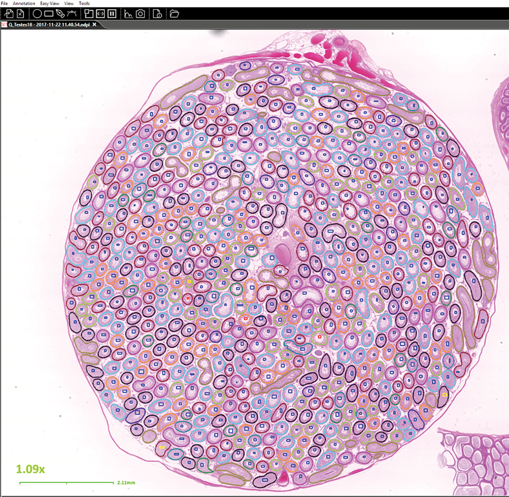
Tubules annotated by the algorithm and pathologist during validation of the algorithm. Each appropriately sectioned tubule was outlined using a different color, depending on the stage identification assigned by the algorithm. The pathologist then examined each annotated tubule and added an additional rectangular box annotation in the center of the tubule to confirm or correct the algorithm result. Blue rectangle = pathologist agrees with the algorithm result. Red rectangle = pathologist disagrees with the algorithm result. Yellow rectangle = pathologist considers the tubule inadequate for staging.
Algorithm Development: Technical Details
The staging algorithm was developed using deep learning and machine learning methods based on those described by Ronneberger et al
5
and Song and Lu.
7
Our approach for automated staging was broadly categorized into 3 steps: Segmentation of individual tubules at 10× magnification, stitching the 10× results at 2.5× magnification, and then mapping them to 40× magnification. Segmentation of the lumen and various germ cells (Spg, Spcs, RSps, and ESps), MFs, and RBs from the mapped tubules at 40×. Generation of a 28-dimension feature vector corresponding to each tubule and then training a decision tree-based classifier using the feature matrix obtained thereon.
These steps are explained in more detail below.
Step 1
In the first step, accurate semantic segmentation of the seminiferous tubules was carried out by training a U-Net-based deep learning model on the tiles from the training data set. The corresponding labeled tiles were generated by labelling the data for 3 classes, that is, 1 label for the content inside the tubule, second label for the content outside the tubule, and the third label for the periphery of the tubule. The reason behind such a labelling was to segment out the touching tubules separately. For training of the tubule segmentation model, a total of 1500 tiles at 10× magnification were selected from the development data set by taking 1125 tiles from the training data set (15 WSIs) and 375 tiles from the test data set (5 WSIs). The training setup is discussed below in the Algorithm Training section. The trained model was then tested on the tiles from 13 WSIs from the validation data set. As a single tile generally contained more than one tubule and some tubules were not complete at tile level, we stitched the 10× segmented output tiles together at 2.5× magnification. Tile stitching was performed at 2.5× magnification to avoid memory constraints in stitching a full image at 10× magnification due to its larger size. The individual connected components (tubules) were then mapped and saved at 40× magnification to detect the various germ cells present.
Step 2
In the second step, the lumen, various germ cells, and RBs were segmented out. Here, the lumen (at 10× magnification) and various germ cells (at 40× magnification) were segmented out using U-Net-based deep learning models, whereas the RBs were segmented out by using image processing-based methodology. The lumen was labeled in such a way that the RBs of stages VII and VIII were included as a part of the lumen. For training the lumen segmentation model, a total of 783 tiles at 10× magnification were selected from the development data set by taking 587 tiles from the training data set and 196 tiles from the test data set. The output tiles of the lumen segmentation model were stitched together at 2.5× magnification and mapped to 40× magnification, corresponding to individual tubules. The image processing method employed to segment out RBs was applied only to the lumen output.
Two models were used to segment out the different germ cells and meiotic bodies. The first model is a 6-class model where the germ cells segmented out were RSps (stage I to stage IX [round spermatids in stage IX = step 9 spermatids that are just starting to elongate] and stage XIV [round spermatids in stage XIV are step 1 spermatids that may or may not be present following the final meiotic division of secondary Spcs]), elongating spermatids (stage X), Spg (wherever present), Spcs (pachytene and secondary Spcs, wherever present), and MFs (wherever present). For training this 6-class model, a total of 881 tiles at 40× magnification were selected from the development data set by taking 661 tiles from the training data set and 220 tiles from the test data set. The second model is a binary model where elongated spermatids (stage I-stage VIII and stage XI-stage XIV) were segmented out. For training this binary model, a total of 788 tiles at 40× magnification were selected from the development data set by taking 591 tiles from the training data set and 197 tiles from the test data set. After accurate detection of germ cells, they were mapped onto corresponding tubules at 40×.
Step 3
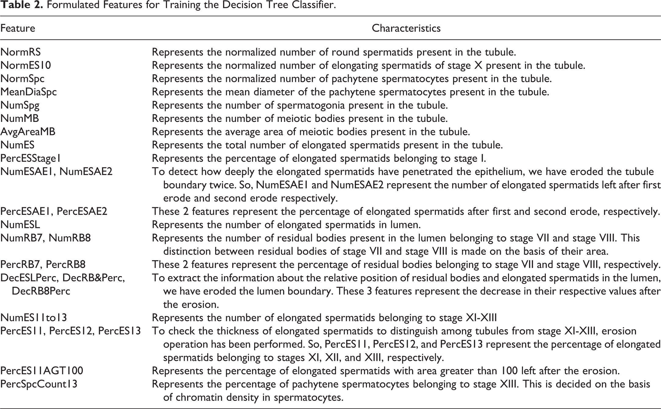
In the third step, a feature vector of 28 dimensions was created, corresponding to each tubule present in the development data set and the validation data set. A total of 9204 tubules were present in the 20 WSIs of the development data set and 7502 tubules were present in the 13 WSIs of the validation data set. The features corresponding to each tubule were formulated based on presence or absence of certain germ cells along with their morphological features such as shape, size, and relative position as described in Table 1. The formulated features that were developed for training the decision tree classifier are provided in Table 2. A feature matrix of dimension 9204 × 28 was obtained for the tubules present in the development data set and a decision tree classifier was trained using this feature matrix. The training setup for the decision tree classifier is described below in the algorithm training section.
Formulated Features for Training the Decision Tree Classifier.
Algorithm Training: Technical Details
Four U-Net-based deep learning models were trained to segment out the various parameters. In summary, one model was trained for tubule segmentation (3 class models), 1 for lumen segmentation (2 class models), 1 for ESp segmentation (2 class models), and 1 for other germ cells (6 class models), as mentioned in the Algorithm Development section. The exact architecture of the deep learning model is as shown in Figure 3. The network comprises downsampling and upsampling information flow with 31 convolution layers, 4 transpose convolution layers, and 1 up-sampling using nearest neighborhood. Similar to U-Net architecture, skip connections are added in the network to ease the optimization during backpropagation of gradients, hence eliminating the vanishing gradient problem. In this network, we incorporated a multipath branched module, namely an inception module 10 for multiscale processing of features in the encoder layer of the vanilla U-Net 5 architecture as shown in Figure 4. Beside this, we have also introduced a residual-bottleneck module 11 in the decoder layer to increase the resolution and reduce the feature dimension as shown in Figure 4.
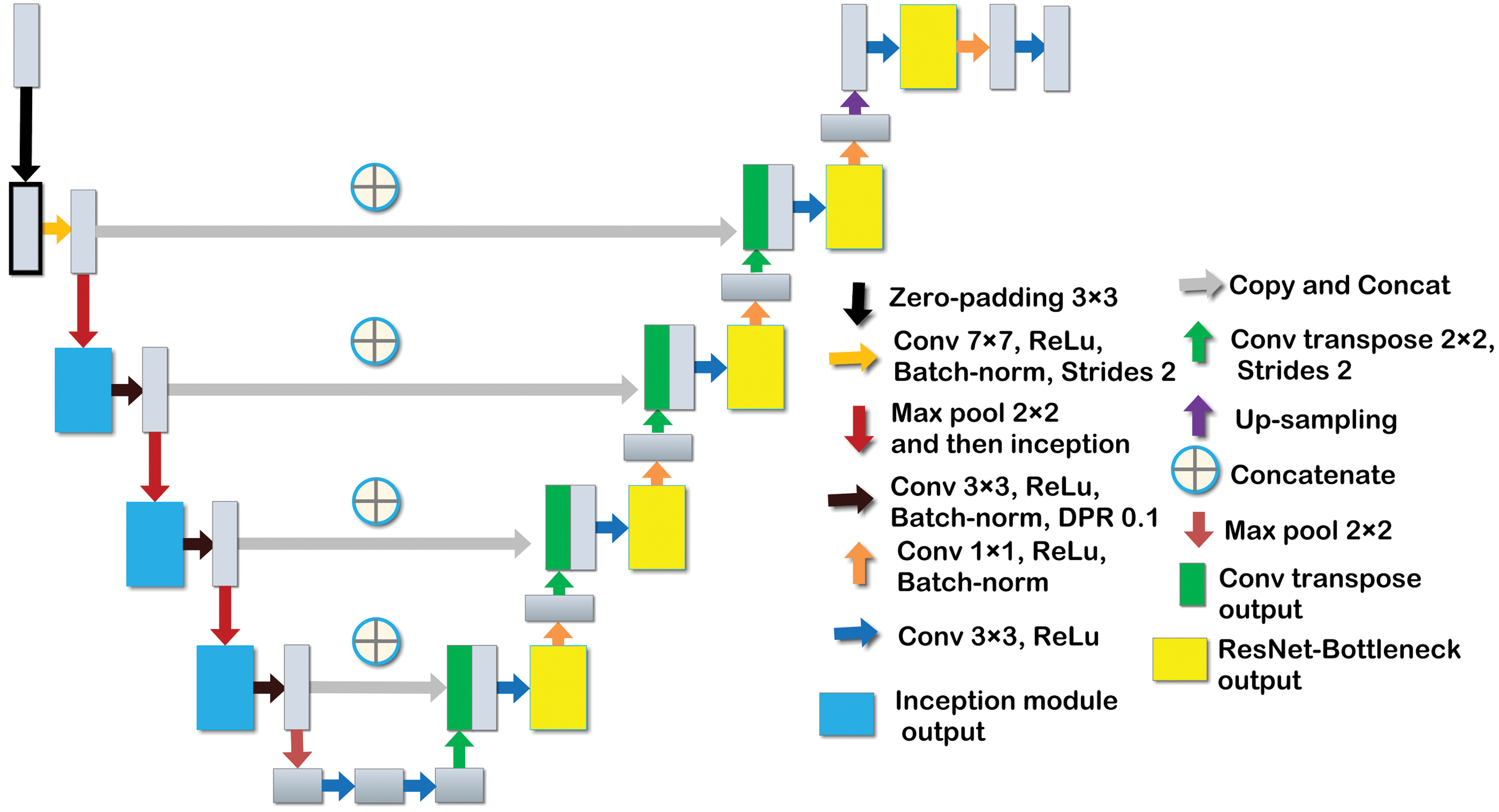
Network architecture of modified U-NET used for semantic segmentation of various parameters.
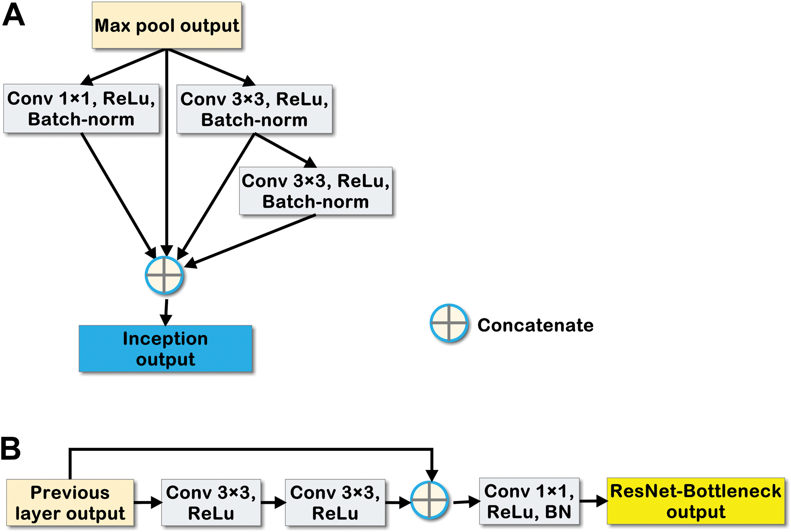
Structure of (a) the inception module which is used for multiscaling of features in the encoder layer of vanilla U-NET architecture. b, Structure of ResNet-bottleneck module which is used to increase the resolution and reduce the feature dimension in the decoder layer of vanilla U-NET architecture.
To train these models, tiles were selected from the training data set (75% of total tiles) and the test data set (25% of total tiles). The model was developed in Keras framework with tensorflow-backend where we have used Adam as an optimizer, categorical cross-entropy as a loss function, batch size of 8, and learning scheduler to set the learning rate. During training, the starting learning rate was 0.001 and it was increased 1 decimal place for every 200 epochs. Every convolution layer was initialized by Xavier initializer and every layer was followed by a batch-normalization layer. Using the above-mentioned training setup, the model was trained until it was converged, where validation loss was incorporated to monitor the convergence. After the segmentation of all the parameters, the tile-level results at 10× magnification (results from tubule and lumen segmentation models) were mapped to 40× magnification and then all the results at 40× magnification (including the results from the other 2 models) were saved tubule wise to extract the 28-dimensional feature vector corresponding to each tubule.
Secondly, a decision tree was incorporated to classify the tubules into 10 pooled stages. A decision tree is a supervised machine learning algorithm mainly used for classification problems. It is simply a series of sequential decisions made to reach a specific result. So, it makes a series of decisions based on a set of features present in the data, which in our case were count, position, shape, and size of various germ cells. The sequence of attributes to be checked is decided, on the basis of criteria like Gini impurity index (used in our case) or information gain. All decision trees need stopping criteria. There are a number of stopping criteria, namely maximum depth of the decision tree (=18 in our case), minimum samples at the node for further split (=2 in our case), minimum samples in the leaf node required for a split (=1 in our case), and so on. This decision tree classifier was trained using scikit-learn libraries in python. The learning and decision making by the trained decision tree classifier are similar to those pathologists consider while deciding on a particular stage. For example, stage XIV has 455 instances in the training data and the majority of the instances (327) have followed the decision path as shown in Figure 5. The entire decision tree is too large to illustrate in its entirety, but Figure 5 shows a branch of the decision tree classifier. Here the classifier decides, based on the presence of meiotic bodies and whether there are RSps and elongated spermatids belonging to stage I. These are the same features that a pathologist uses to make a decision when classifying stage XIV tubules.
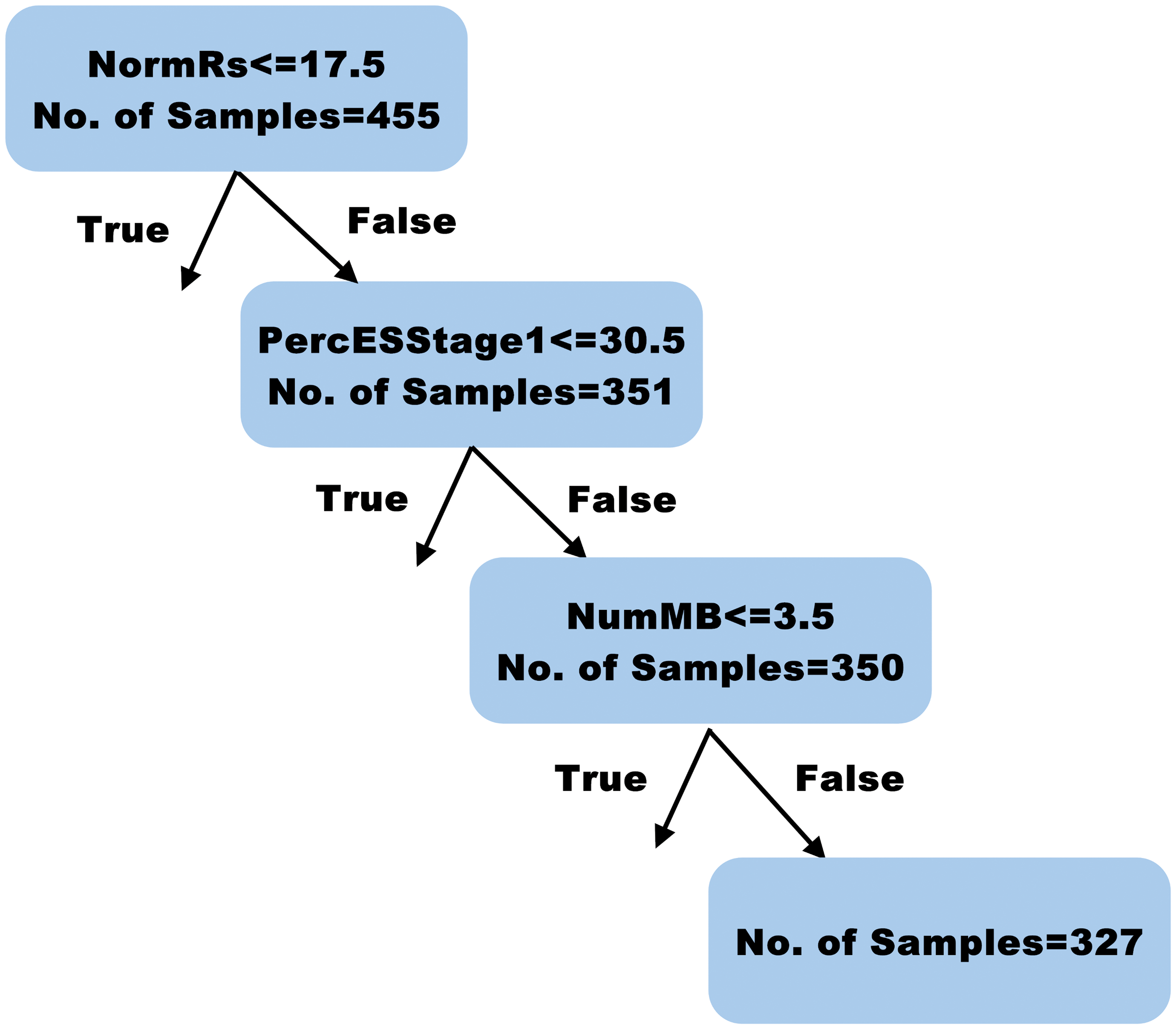
One of the branches of the trained decision tree classifier that shows 1 set of the decisions taken to classify a stage XIV tubule. The decisions learned by the classifier are similar to the ones that a pathologist takes.
Algorithm Validation
We validated our trained algorithm on 13 WSIs from the validation data set. We used the same procedures as during the training phase, whereby the algorithm-generated staging annotations for each appropriately sectioned tubule were reviewed by the same pathologist as in the training phase but in this case, the pathologist either confirmed their agreement with the algorithm stage or disagreed and added an annotation providing the corrected stage. We used these data to generate a confusion matrix and from this table, we calculated the various performance metrics for the algorithm when compared with the pathologist. In addition, we generated a stage frequency map for the algorithm and pathologist-generated results and compared this with the stage frequency map for PAS-stained rat testes published by Hess et al. 9
Data Handling and Generation of Performance Metrics
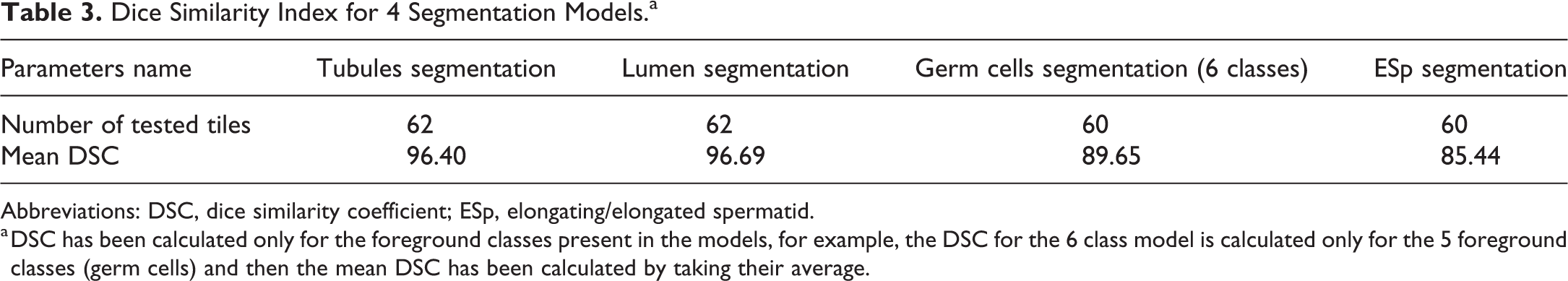
To evaluate the performance of semantic segmentation, we calculated the dice similarity coefficient (DSC) for all the segmentation models. Dice similarity coefficient has been adopted to validate the segmentation results. The value of a DSC ranges from 0, indicating no spatial overlap between ground truth and predicted output, to 1, indicating complete overlap between the 2 sets. Dice similarity coefficient is calculated by the formula: DSC = 2 × (overlapped region between ground truth and predicted output)/(union of ground truth and predicted output). Dice similarity coefficient for the 4 segmentation models is as shown in Table 3. Dice similarity coefficient has been calculated only for the foreground classes present in the models, for example, the DSC for the 6 class model is calculated only for the 5 foreground classes (germ cells) and then the mean DSC has been calculated by taking their average.
Dice Similarity Index for 4 Segmentation Models.a
Abbreviations: DSC, dice similarity coefficient; ESp, elongating/elongated spermatid.
a DSC has been calculated only for the foreground classes present in the models, for example, the DSC for the 6 class model is calculated only for the 5 foreground classes (germ cells) and then the mean DSC has been calculated by taking their average.
To evaluate the performance of the decision tree classifier, we calculated the precision, recall (sensitivity), and f1-score corresponding to each stage. The combined data for all stages was then used to calculate the overall accuracy of the algorithm when compared with the pathologist. Below are detailed definitions for the performance parameters: True positive (TP): When a positive sample annotated by the pathologist is truly predicted as positive by the algorithm. For example, when a stage I tubule is predicted as stage I by the algorithm. True negative (TN): When a negative sample annotated by the pathologist is truly predicted as negative by the algorithm. For example, when a nonstage I tubule is predicted as a stage other than stage I by the algorithm. False positive (FP): When a negative sample annotated by the pathologist is falsely predicted as positive by the algorithm. For example, when a nonstage I tubule is predicted as stage I by the algorithm. False negative (FN): When a positive sample annotated by the pathologist is falsely predicted as negative by the algorithm. For example, when a stage I tubule is predicted as a stage other than stage I by the algorithm. Precision: Precision is a measure that tells us what proportion of instances detected by the algorithm as positives, were TPs, that is, precision = TP/(TP + FP). Recall or sensitivity: Recall is a measure that tells us what proportion of instances that actually were positives, were detected by the algorithm as positives, that is, recall = TP/(TP + FN). F1 score: F1 score combines both precision and recall using the harmonic mean. F1 score = 2 × precision × recall/(precision + recall). A high value of f1 score represents a high value for both precision and recall. Accuracy: Accuracy is defined as the percentage of correctly classified instances, that is, (TP + TN)/(TP + TN + FP + FN).
Results
Development and Training of the Algorithm
During the initial assessment and training phase of the project, it became apparent that the basic criteria used by Creasy and Chapin 4 were insufficient on their own to allow automated digital methodology to differentiate between stages. Their basic criteria rely predominantly on the shape and position of the ESps as they move through the tubular epithelium. Additional criteria, including the size and appearance of the accompanying Spcs, the relative numbers of Spg, and the size and position of the RBs, were additional important features that were incorporated into the algorithm. The main criterion used to identify early stage tubules (stages I-VI) was the position of the elongated (step 15-18) spermatid heads as they move from the lumen in stage I, down through the epithelium during stages II and III, arriving at the base of the epithelium in stages IV and V, and then moving back up through the epithelium during stage VI (Figure 6A-D). Not all elongated spermatids move at the same rate and so there is some inconsistency in the level that each bundle reaches within a tubule. Although the pathologist can overcome this inconsistency by making a subjective decision on where the majority of the spermatid heads are positioned, an algorithm requires more precise features or additional criteria to make an accurate stage determination. For this reason, additional morphologic features including the relative diameter of the pachytene Spcs and the relative numbers of Spg were used to improve the staging accuracy of the early stages. Due to the difficulties outlined above, it was found necessary to combine some of the early stages to achieve adequate precision and accuracy. Therefore, stages II and III, IV-VI, and XII and XIII were combined. The features of the different stages are illustrated in Figures 6, 7, and 8.
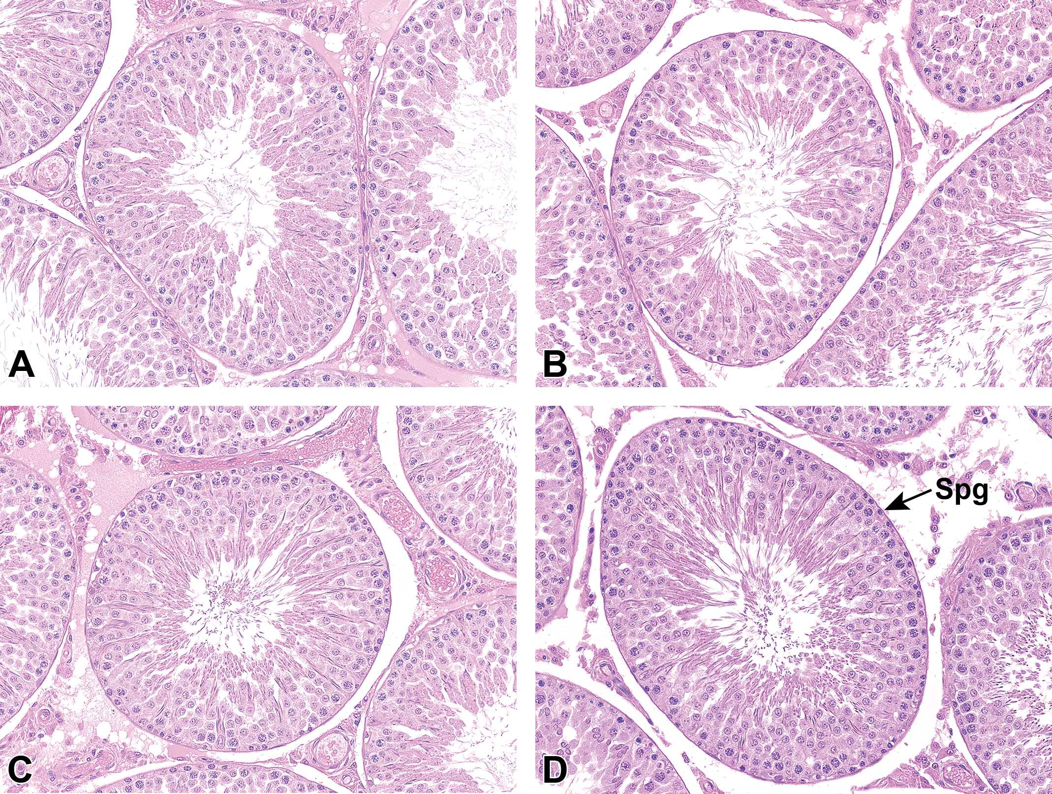
Histological appearance of tubules in stages I, II/III, and IV-VI. A, Stage I: ESp heads are close to the lumen and show limited bundling. B, Stage II/III: ESp heads have started descending toward the base of the tubule in bundles. C, Stage IV-VI (mid): Most ESp heads are bundled and close to the tubule base. D, Stage IV-VI (late): ESp heads are starting to return toward the lumen and there are increased numbers of B spermatogonia (Spg) compared with stage II/III. H&E stain. ESp indicates elongating/elongated spermatid; H&E, hematoxylin and eosin.
The mid stages (VII and VIII) were identified and distinguished from one another, largely by the presence, position, and size of the RBs (Figure 7A-D). For the later stages (stages IX-XIII), the shape of the elongating (step 9-13) spermatid heads was the main criterion used (Figure 8A-E). Due to the fact that not all of the spermatid heads in a tubular cross section will change shape at the same time, there was an element of variability in staging these later stages. In addition, it was difficult to clearly delineate the boundary between stage XII and XIII based on the changing shape of the elongating spermatid head and the relative size of the pachytene Spc and so these 2 stages were combined (Figure 8D and E).
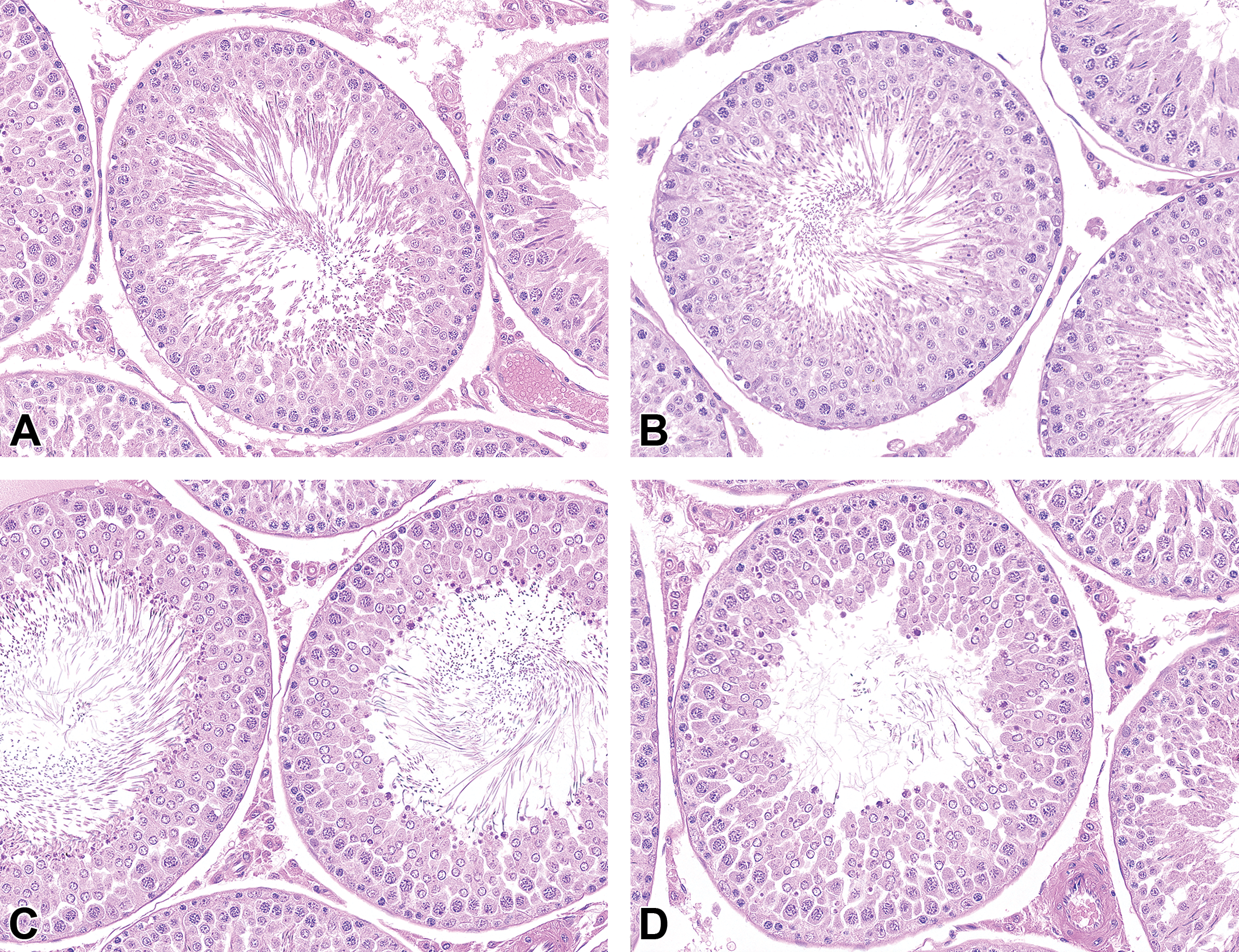
Histological appearance of tubules in stages VII and VIII. A, Stage VII (early): ESp heads are all at the lumen but RB formation is rudimentary. This tubule is transitioning from stage VI. B, Stage VII (mid) ESp heads at the lumen with small RBs above and below ESp heads. C, Stage VIII: left tubule is early stage VIII with large RBs around head of ESp. Right tubule is late stage VIII with large RBs below ESp heads and reduced numbers of ESp (due to partial release). D, Transition between stage VIII and IX. Most but not all ESps have been released but RBs are still at the lumen and RSps are just beginning to lose their round profile. H&E stain. ESp indicates elongating/elongated spermatid; H&E, hematoxylin and eosin; RB, residual body; RSps, round spermatid.
Stage XIV can have a very variable appearance depending on whether it is at the beginning, middle, or end of the stage. At the beginning of stage XIV, the tubule mostly contains large diakinetic Spcs, while in the middle of the stage (Figure 8F), it contains a variable mixture of diakinetic Spcs, secondary Spcs, and RSps, whereas at the end of the stage, it contains almost all RSps. The only reliable feature is the presence of at least 1 MF in the dividing primary or secondary Spcs and so this was used as the primary criterion for stage XIV.
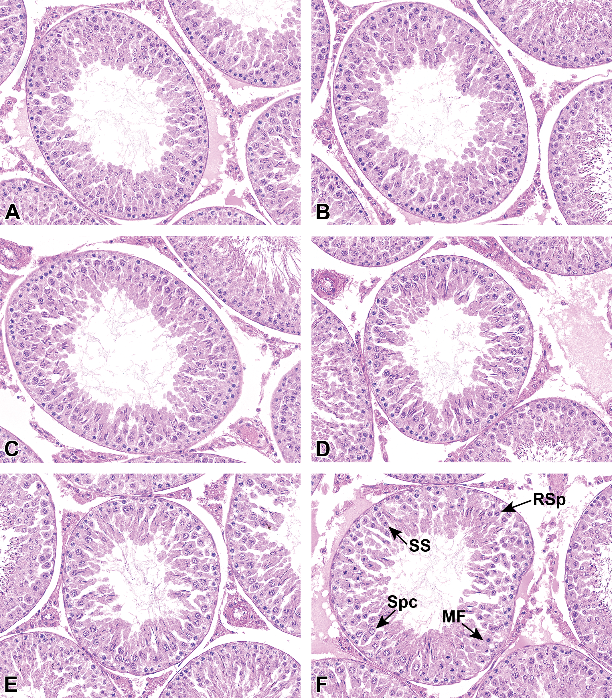
Histological appearance of tubules in stages IX, X, XI, XII/XIII, and XIV. A, Stage IX: RSps are just starting to become elliptical, RBs are mostly at the base. B, Stage X: ESps are mostly elliptical (but note the variable shape). C, Stage XI: ESps are mostly banana shaped. D, Stage XII/XIII (early): ESp heads have condensed and lengthened to form a scimitar shape. E, Stage XII/XIII (late): ESp heads are very thin and thread-like and the pachytene spermatocytes are enlarged with sparse chromatin. F, Stage XIV (mid): tubule contains diakinetic Spc, SS, RSps, and MF. H&E stain. ESp indicates elongating/elongated spermatid; H&E, hematoxylin and eosin; MF, meiotic figures; RB, residual body; RSps, round spermatid; Spcs, spermatocytes; SS, secondary spermatocytes.
Particular problems were encountered when tubules were transitioning between consecutive stages and contained features of both stages. This made it difficult to establish user-defined thresholds on various staging parameters, so it was necessary to automate this. Hence, we trained a decision tree classifier on the 28-dimensions feature vectors using methodology based on Song and Lu. 7
Validation of the Algorithm
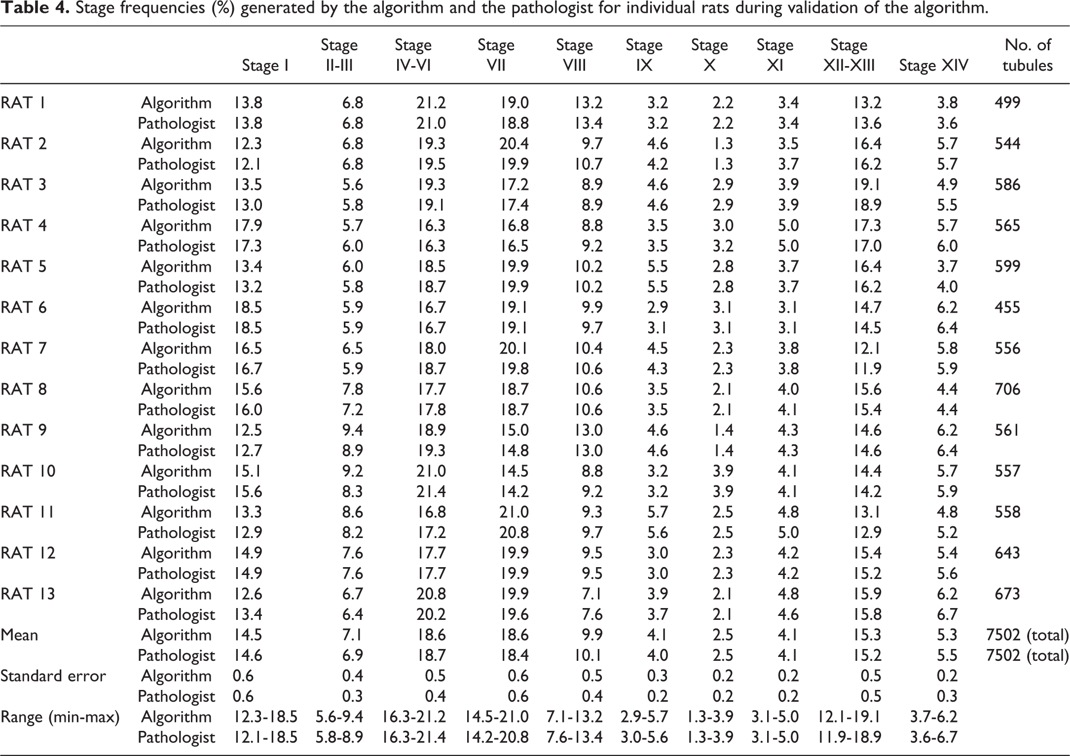
Once the staging criteria had been improved and finalized using the initial set of 20 testis images, the validation of the algorithm was performed on a further set of 13 testis images. In this study, we only included nearly round tubules for staging analysis. We excluded those tubules sectioned longitudinally because they often comprise more than one stage and are frequently sectioned tangentially. From the 13 testis images, we obtained 7502 tubules that met the qualifying criteria for staging analysis. As mentioned earlier, we pooled some of the stages leaving us with 10 different classifications, that is, stages I, II-III, IV-VI, VII, VIII, IX, X, XI, XII-XIII, and XIV. All the tubules were then classified in one of the above-mentioned categories by the algorithm, and these results were confirmed or refuted by the pathologist (Table 4). After the algorithm was run on all the tubules, we generated a confusion matrix, which describes the performance of a classification model on a set of test data for which the true values are known (in this case, the true value being the stage called by the pathologist). From this confusion matrix, we then calculated the various performance metrics, that is, precision and recall. Precision refers to what proportion of the positive identifications made by the algorithm was actually positive (according to the pathologist), while recall refers to what proportion of the actual positives (according to the pathologist) was called positive by the algorithm. Both the parameters, in some sense, represent the accuracy of the algorithm. For a good classification model, both precision and recall should be high; f1 score gives the combined information about the precision and recall of a model such that a high value of f1 score indicates high value for both precision and recall. Comparison of the staging results obtained by the algorithm versus those obtained by the pathologist is presented in the confusion matrix in Table 5 and the performance metrics for the algorithm in Table 6. Precision was ≥0.93, recall was ≥0.96, and f1-score was ≥0.94 (all stages considered), with overall accuracy of the staging algorithm being 0.984. The performance metrics demonstrate that there was very good agreement between the staging results of the algorithm and the pathologist. This was true for all the different stages evaluated. Table 5 demonstrates that for the few tubules where there was a difference in stage identification, the difference was largely restricted to ±1 stage.
Stage frequencies (%) generated by the algorithm and the pathologist for individual rats during validation of the algorithm.
Confusion Matrix for Staging Results From Pathologist Versus Algorithm.a
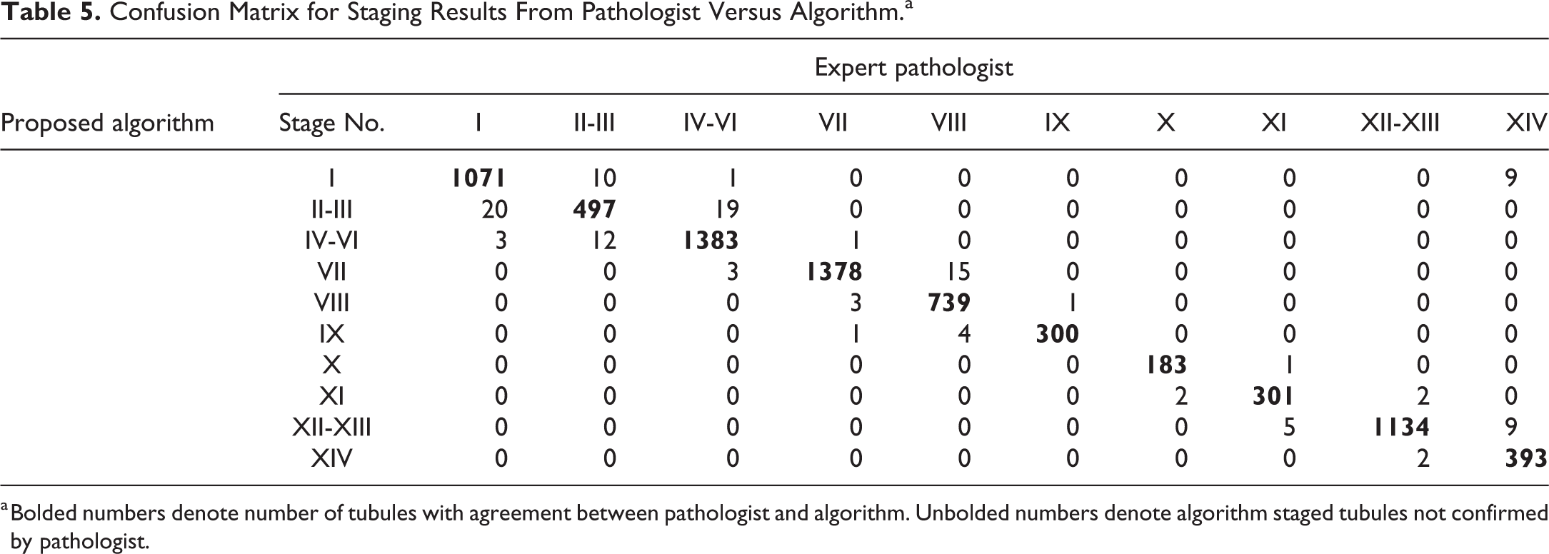
a Bolded numbers denote number of tubules with agreement between pathologist and algorithm. Unbolded numbers denote algorithm staged tubules not confirmed by pathologist.
Stage-Wise Performance Metrics of the Algorithm.
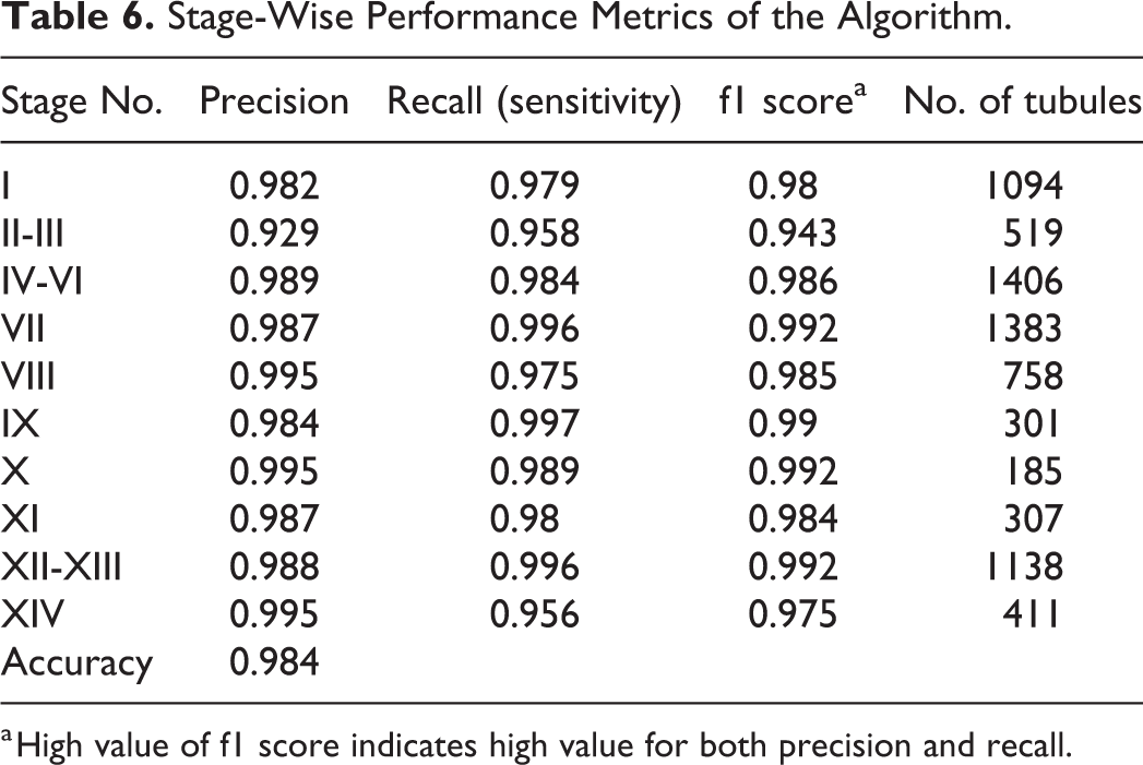
a High value of f1 score indicates high value for both precision and recall.
Comparison of Stage Frequency (%) Distribution in H&E-Staged Testes by the Algorithm and the Pathologist With Published Stage Frequencies in PAS-Stained Testes 9,a.
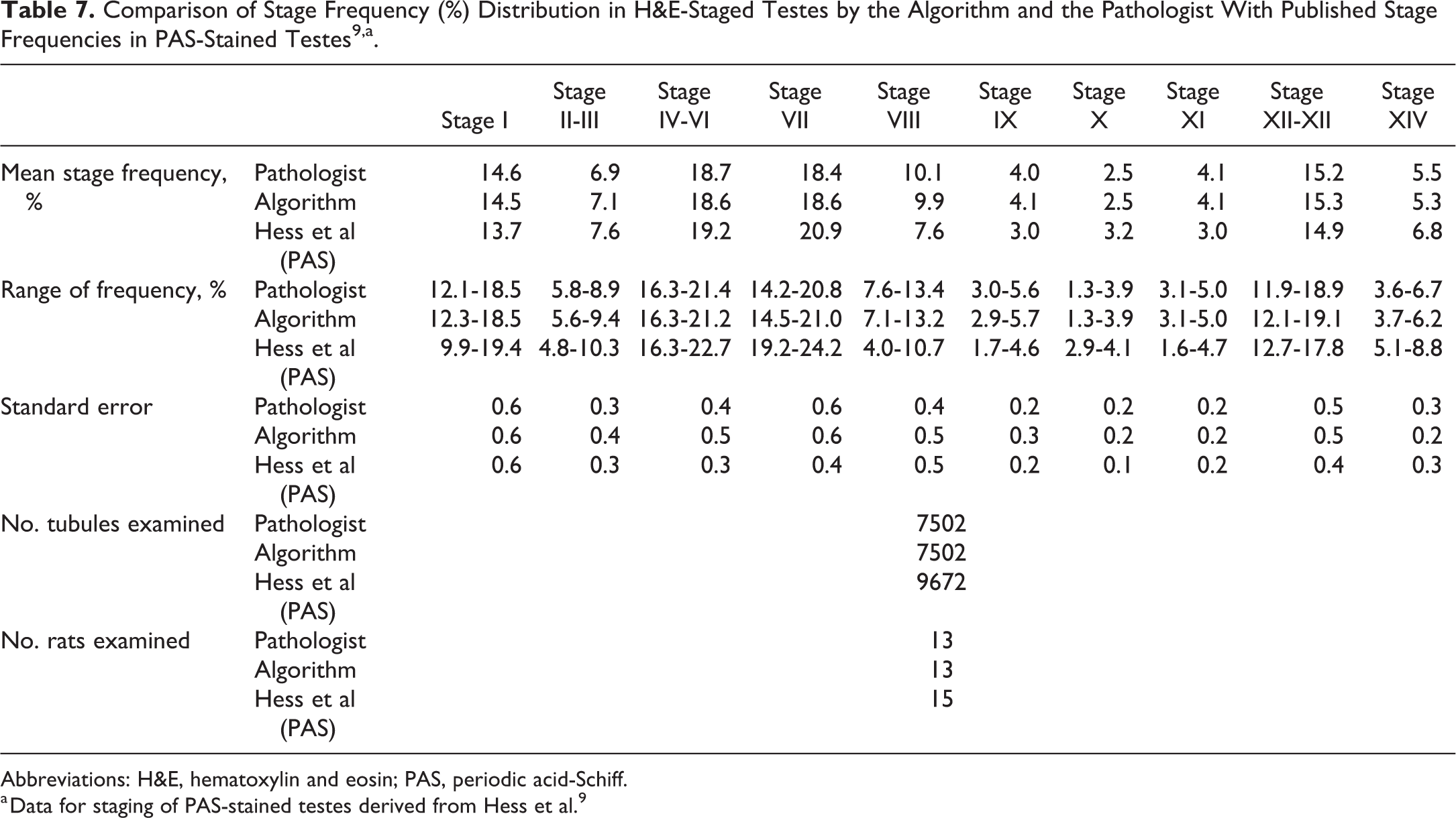
Abbreviations: H&E, hematoxylin and eosin; PAS, periodic acid-Schiff.
a Data for staging of PAS-stained testes derived from Hess et al. 9
To confirm that the staging criteria that we developed for the H&E-stained testes provided similar stage frequencies to those obtained from PAS-stained testis sections, we generated staging frequency tables using the data generated by the pathologist and the algorithm on the 13 testes (7502 tubules) used in the validation study. This was compared with the stage frequencies published by Hess et al 9 who staged 15 PAS-stained testes (9,672 tubules) from Sprague-Dawley rats. The results are detailed in Table 7 and illustrated in Figures 9 and 10. Figure 9 illustrates the stage frequency comparison between the algorithm and the pathologist in the form of box plots, whereas Figure 10 illustrates this comparison plus the data from Hess et al, in the form of bar graphs. The mean frequencies for the different stages were broadly similar between the data sets, as was the individual variation (range) of frequencies for the same stage between individual rats
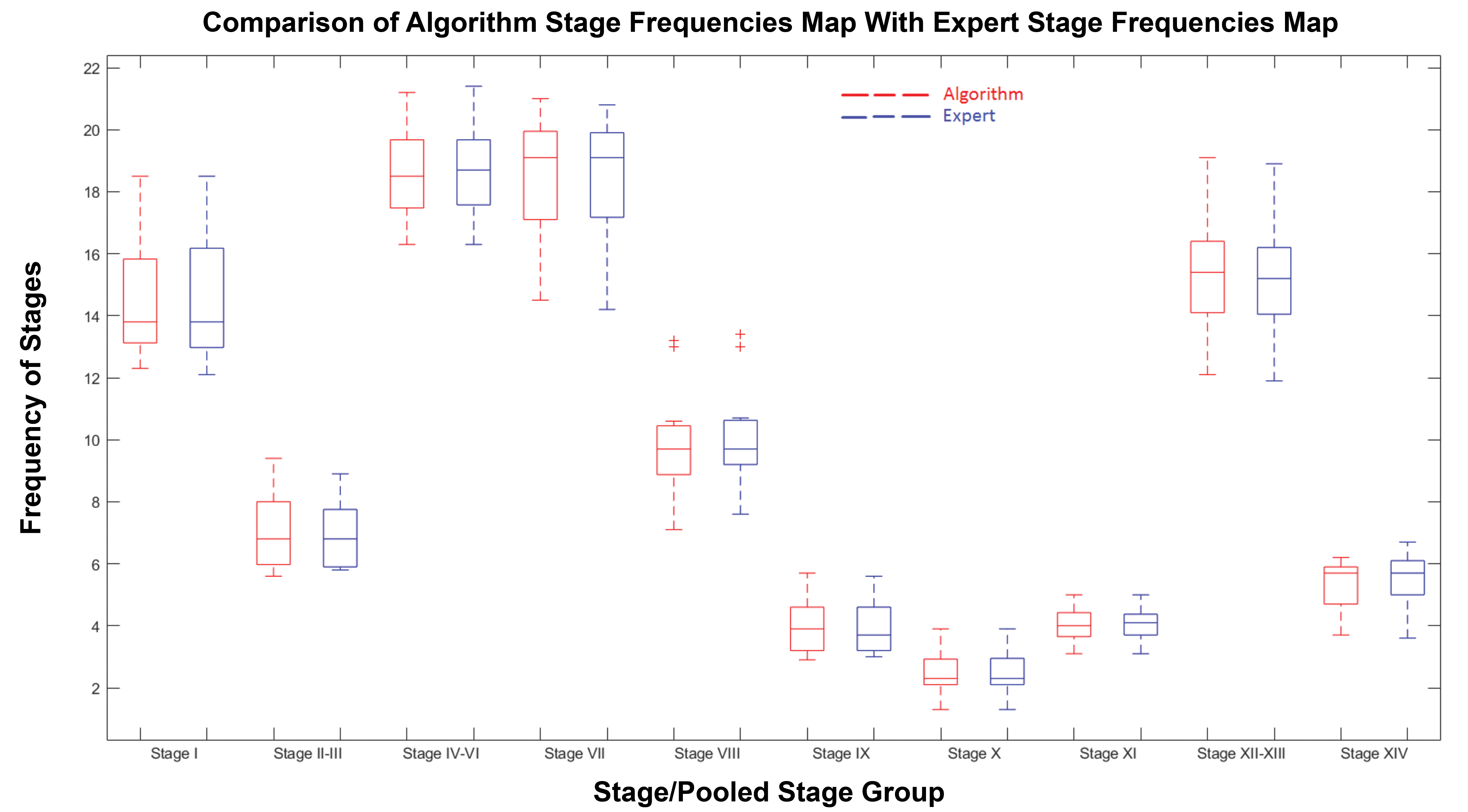
Boxplot for the comparison of algorithm stage frequencies (%) with pathologist stage frequencies (%).
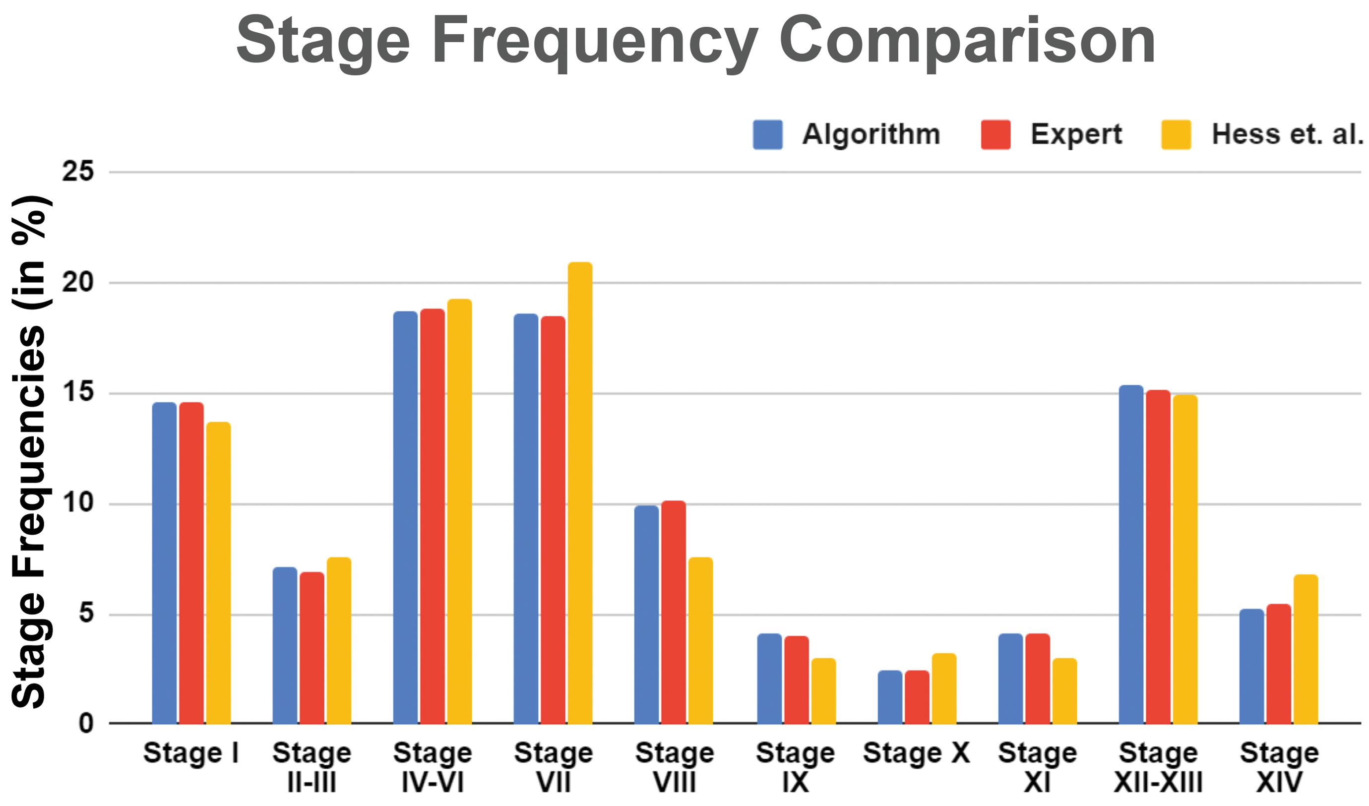
Stage frequency following staging by pathologist and algorithm in H&E-stained testes, compared with stage frequency in PAS stained. H&E indicates hematoxylin and eosin; PAS, periodic acid-Schiff.
Discussion
Development of Staging Criteria for H&E-Stained Testes
Criteria for staging H&E-stained testes have previously been published. 4 The published criteria utilize the changing shape and movement of the elongating spermatid (step 14-19 spermatids) within the seminiferous epithelium, along with the size of the RB to distinguish between stages I-VIII. For stages IX-XIII, the criteria utilize the changing shape of the elongating spermatid (step 9-13 spermatids), while stage XIV is recognized by the presence of Spcs undergoing meiotic division. Since the stages of the spermatogenic cycle form a continuum and the development of all the spermatids within a stage will not be in complete synchrony with one another, there are always difficulties with deciding where 1 stage ends and the next begins (Figure 7A-D). This is not a significant problem for a pathologist, because they can make a subjective judgment based on what most of the spermatids are doing in a tubule. However, it does present a problem when trying to develop an algorithm based on defined criteria. This proved to be a particular problem for stages I-VIII. To improve the accuracy and precision of the algorithm, additional criteria were introduced that took into account (1) the position of the RBs with respect to the elongating spermatid head, (2) the relative size of the pachytene Spcs, and (3) the relative numbers of Spg around the base of the tubule. The final criteria used by the algorithm for distinguishing between the stages are summarized in Table 1.
Testing for Accuracy and Consistency of Staging and Rationale for Pooling Stages
During development of the algorithm, we needed to confirm that the H&E method of staging conformed adequately with the PAS method of staining (which is considered the “gold standard”). To do this, we compared the stage frequency data obtained by the pathologist and the algorithm with the published stage frequency data for PAS-stained testes. 9 Even using the enhanced criteria described above, certain stages proved difficult to separate with acceptable consistency (both by the pathologist and by the algorithm). For example, stage II and III are identified by the presence of bundles of ESp heads descending toward the base of the tubule, which they do at variable rates. So, there is no distinctive feature to separate stage II from III. During stage IV, V, and VI, the ESp heads are arriving at the base of the tubule and then starting to ascend back to the surface. However, we could not separate these 3 stages with an acceptable degree of consistency. Similarly for stage XII and XIII, it proved difficult to distinguish consistently between the shape of the ESp heads in the two stages. Accuracy and consistency were assessed on the basis of the stage frequency data generated from the staging results of the algorithm and of the pathologist (Figure 9) and comparing them with the mean, range, and standard error data published by Hess et al 9 for PAS-stained sections (Table 7 and Figure 10). To alleviate this problem, certain stages (II-III, IV-VI, and XII-XIII) were pooled. Once these stages were pooled and compared with the data from Hess et al, 9 the overall mean frequency for each group of stages was similar, as was the standard error and the range of frequencies of a given stage between animals. Hess et al performed his assessment on Sprague-Dawley rats whereas this study used Wistar rats. Although mean stage frequency differs slightly between strains, they are broadly similar.
For the purpose of screening testes for abnormalities, such as the presence or absence of specific populations of germ cells, this pooling is not considered a problem because the makeup of these adjacent stages is very similar. However, if changes were observed in a specific cell population of these pooled stages and accurate stage specificity of the change was required, it may be necessary to perform a PAS stain to establish the exact stage(s) affected.
Performance Metrics of the Algorithm
The performance metrics for the algorithm results versus the pathologist results (Table 6) shows very good agreement for all the stages with precision, recall, and F1-score being ≥0.93 and ≥0.96 and ≥ 0.94, respectively, and overall accuracy of the staging analysis was 0.984. Differences between the algorithm and the pathologist diagnosis were generally limited to ± 1 stage (Table 5), and most of the differences were in the early part of the cycle (stages I-VI). The difficulties in distinguishing these early stages are due to the inconsistent rate at which the elongated spermatids descend from the lumen to the base of the tubule and then return. For example, in stage II/III, the elongating spermatid heads will begin to form bundles and will start to descend toward the base of the tubule. However, in a given cross section of tubule, a few will have already reached the base and a few will still be at the lumen, so the stage is decided on the basis of where the majority of the spermatid heads lie (Figure 6B). The same is true when staging PAS-stained testes, where the developing acrosomic granule in the RSp is the main criterion used for staging. A proportion of spermatids will show the feature while others will not. In addition, since the spermatogenic cycle represents a continuous morphological development of germ cell features, identifying where 1 stage ends and the next begins is a subjective decision and not a precise event, and so many of the tubules that were transitioning between 1 stage and the next provided a source of variability between the pathologist and the algorithm. Even the same transitional tubule (eg, stage VI/VII as shown in Figure 7A) could be staged as VI on 1 occasion and stage VII on another occasion by the expert pathologist. To minimize the impact of this subjectivity on the final assessment of the algorithm, it was decided that during the validation stage of algorithm development, the pathologist would decide whether they agreed with the algorithm annotation rather than provide a separate (subjective) “blinded” annotation. Based on this assessment, the performance metrics of the algorithm versus the pathologist and the similarity of the stage frequency map between the H&E-stained testes and the published frequencies of PAS-stained testes indicate that this automated staging program provides an acceptable substitute for manual staging of testes.
Utility of Automated Staging for the Pathologist
The usefulness of the automated technique lies in its ability to provide the pathologist with a digital map of a transverse section of testis that is annotated with the stage of spermatogenesis for each tubular cross section. Some regulatory guidelines specifically recommend that testes should be examined with an awareness of staging so that subtle changes in germ cell populations or spermatid retention can be recognized (reviewed by Lanning et al). 1 In addition, the STP recommendations for examination of testes and epididymides recommend that testes from all shorter-term studies should be examined with an awareness of staging. 1 This generally necessitates staining an additional section of testis with PAS stain followed by a specially trained pathologist performing the examination. This automated staging program is designed to be used on routine H&E-stained sections and will provide an image of the testis, ready annotated with the stage of each tubule. With such an annotated image, the pathologist can readily evaluate the testis with an “awareness of staging,” as recommended by the guidelines. However, it is essential that the pathologist understands the underlying histological basis and the dynamics of staging so that they are able to recognize abnormalities within the staged seminiferous tubules, because the algorithm will not do this for them. An example of its usefulness would be for the detection of spermatid retention. This is a subtle but important change characterized by the inappropriate presence of step 19 spermatids (which should be released in stage VIII) still being present in stages IX-XII. Tubules in these stages could be rapidly identified, selected, and examined by the pathologist for the abnormality. However, it requires that the pathologist understands what step 19 spermatids look like and know that they should not be present in stage IX-XII tubules. Another example would be if a cell population such as pachytene Spcs was degenerating or depleted from stage VII tubules. The pathologist needs to recognize that there is an abnormality, that is, that germ cells are degenerating or depleted, but the algorithm would be able to identify which stage they were in and would be able to select all remaining stage VII tubules so that the pathologist could easily examine them.
Analysis of individual stage frequency could also be performed very easily. The frequency of an individual stage or pool of stages is proportional to the duration of the stage(s). Therefore, if the frequency of a stage significantly increases (compared with control values), it would suggest that the duration of the stage had increased. Similarly, if the frequency of a stage decreases, it would suggest a decreased duration of the stage. Although such a disturbance in the dynamics of the spermatogenic cycle by a toxicant is a theoretical possibility, the authors do not know of any published reports where this has been demonstrated. However, it is also unusual for such a quantitative analysis to be performed as a routine procedure. Although the authors would not recommend performing a stage frequency analysis as a routine procedure for a regulatory toxicity study, it is a rapid and useful tool that could be employed if the pathologist has an impression that a certain stage (eg, stage XIV) is more or less common in the test article-treated animals than in the control. So, stage frequency analysis should be considered more of an investigative tool than a routine procedure.
The algorithm in its present format is a valuable tool to the pathologist for automatically identifying stages of spermatogenesis. However, this work could be extended to develop the algorithm to identify subtle, stage-specific degeneration or absence of germ cells, as well as the inappropriate presence of germ cells (eg, spermatid retention) that might be caused by testicular toxicants.
Footnotes
Acknowledgments
The authors would like to thank WuXi AppTec (Suzhou) Co, Ltd, China, for their assistance in preparing and providing the H&E-stained testes slides for this study.
Declaration of Conflicting Interests
The author(s) declared the following potential conflicts of interest with respect to the research, authorship, and/or publication of this article: Rohit Garg and Pranab Samanta are employees of AIRA Matrix, Thane, Maharashtra, India.
Funding
The author(s) received no financial support for the research, authorship, and/or publication of this article.