A hybrid analytical-machine learning framework for data-driven modeling of soliton solutions in the complex Ginzburg-Landau equation

Abstract

The extended complex Ginzburg-Landau equation serves as a fundamental model for nonlinear wave dynamics, governing diverse physical phenomena ranging from particle motion in plasmas to pulse propagation in optical fibers. In this study, we introduce a hybrid analytical-machine learning framework that synergizes traditional mathematical techniques with modern data-driven approaches to comprehensively explore soliton dynamics within this system. First, we employ two advanced analytical methods, the modified Riccati extended simple equation methodology and the new modified generalized exponential rational function approach to derive a rich spectrum of nonlinear wave solutions. These include bright, dark, kink, and combined solitons, alongside hyperbolic, periodic, and exponential function solutions, thereby providing a comprehensive analytical foundation. On these analytical insights we construct a hybrid symbolic-numeric model, implemented by a multilayer perceptron regressor neural network, to find and synthesize soliton solutions to data. The key soliton types such as dark and bright solitons, combined solitons, and periodic solitons are well represented by the proposed framework with high levels of concurrence with the analytical benchmarks as seen by the low error measures. This combination provides a common platform that allows connecting classical analysis methods with modern machine learning, allowing creating as well as effectively simulating nonlinear wave behavior. This work paves the way to the frontiers of the physics of higher dimensional nonlinear waves by demonstrating the utility of this hybrid approach and highlighting some fundamental nonlinear dynamical properties of the model under consideration, and provides a paradigm that can be extended to understand the phenomena involving complex waves in interdisciplinary contexts.

1. Introduction

The study of integrability of any of the forms of nonlinear evolution equations is important in understanding the dynamics of nonlinear waves as well as other related properties. These equations, which characterize time-dependent processes, are often developed from nonlinear partial differential equations (NLPDEs). NLPDEs are now an essential tool for modeling and analyzing natural phenomena in scientific and engineering systems. ¹ Mathematical modeling plays a significant role in the analysis and understanding of physical events by engineers and scientists working in the applied field. ² Solitons, NLPDEs and the Korteweg-de Vries (KdV) equation are concepts that are related to the mathematical sciences. ³ They assist us in comprehension and modeling about the complex systems in nature and engineering. Nonlinear science is the study of disproportionate interactions among variables in a system that can cause chaos, complex patterns and an increase in sensitivity to initial conditions, making it a phenomenon that can result in chaos and complex forms as well as sensitivity of the system to initial conditions. Nonlinear systems can often be meteorology, fluid dynamics and biological systems. NLPDEs are also useful in representing these systems showing how events vary in time and space as nonlinear science is difficult to predict and understand complex systems since relatively small changes can have extremely different impacts. ⁴

It is a balance between nonlinearity and dispersion that allows solitons to exist as localized wave packets that travel long distances without altering their shape or speed. The study of the behavior of waves and the basic ideas of nonlinear dynamics are fundamental to a broad scientific field which includes plasma physics, fluid mechanics, nonlinear optics, and condensed matter physics. ⁵ The KdV equation ⁶ and the nonlinear Schrodinger equation (NLSE) ⁷ are two paradigm models in this area, which are useful in modeling many diverse physical phenomena, including shallow water waves, fibre optical pulse propagation, and the dynamics of BoseEinstein condensates. In contrast to linear partial differential equations (PDEs), where wave packets irreversibly disperse because of dispersion or diffusion, nonlinear evolution equations can support coherent self-reinforcing structures called solitons. The secret of this extraordinary stability is that, nonlinearity cancels dispersive broadening, and solitons can preserve their integrity on arbitrarily long scales. The nonlinear nature of these equations therefore allows us to learn more about the transport of energy, the interactions between waves and how coherent structures arise out of apparently chaotic processes. Solitons are used in numerous technologies, including fusion dynamics, optical coupling deviation, controllers, and sensors.^8,9

In recent years, numerous strategies have been successfully implemented, such as: a novel Jacobi elliptic function expansion technique is employed to investigate a variety of soliton solutions in the (2+1)-dimensional nonlinear electrical transmission line model, as detailed in ¹⁰ . The generalized exponential rational function approach, as described in ¹¹ , is used to study the solitary wave dynamics and interaction phenomena of the ultrasonic model. The fractional resonant Schrödinger equation is examined using the auxiliary equation methodology. ¹² The chaos and sensitivity analyses, together with the solutions to the truncated fractional telegraph equation, are analyzed in ¹³ . The Riccati equation mapping technique has been used to examine Brownian motion inside the stochastic Schrödinger wave equation. ¹⁴ The solitons of the cubic-quartic nonlinear Schrödinger equation have been examined using the Bernoulli G′/G-expansion technique. ¹⁵ The extended nonlinear equation was explored by modified Sardar sub-equation technique. ¹⁶ The neural network approach was applied to extract the exact solutions.^17,18

With recognition of the importance in many domains, we examine in this work the complex Ginzburg–Landau equation and the nonlinear dynamic properties of soliton solutions. This work’s primary innovation is the utilization of sophisticated, innovative techniques to acquire multiple types of soliton solutions by the application of the advanced integration techniques, such as the modified Riccati extended simple equation technique (RMSEM) ¹⁹ and the new modified generalized exponential rational function method (nGERFM). ²⁰ Then, core part of this work is the application of the multilayer perceptron regressor neural network for observing the performance of the soliton solutions. Machine learning improves task performance without explicit programming by identifying patterns in data. In this particular research, the supervised learning is used, and the training models are provided with labeled data, which is divided into training and testing sets to measure the predictive accuracy. Machine learning refers to a revolution in the field of artificial intelligence. It enables computers to learn and become better at data with no explicit programming of each task. Machine learning models can predict and make intelligent decisions by detecting complicated patterns and relationships in the datasets. Its methods include both supervised learning based on labeled data and unsupervised methods based on the discovery of hidden structures.

The findings indicate that the methodologies used are not only beneficial but also strong enough; they can be taken as effective tools having a great impact on engineering and research. The strategies determine substantial results that are progressing in many branches of science and produce new waveforms and solitons. The application of these tools has improved our comprehension of nonlinear dynamics and facilitated the identification of effective solutions. Researchers emphasize the significance of these techniques due to their adaptability; they offer new alternatives for examining nonlinear systems and improve comprehension within that domain. The study has the following sequence as shown in the Figure 1.

Figure 1.

Flow chart of the study.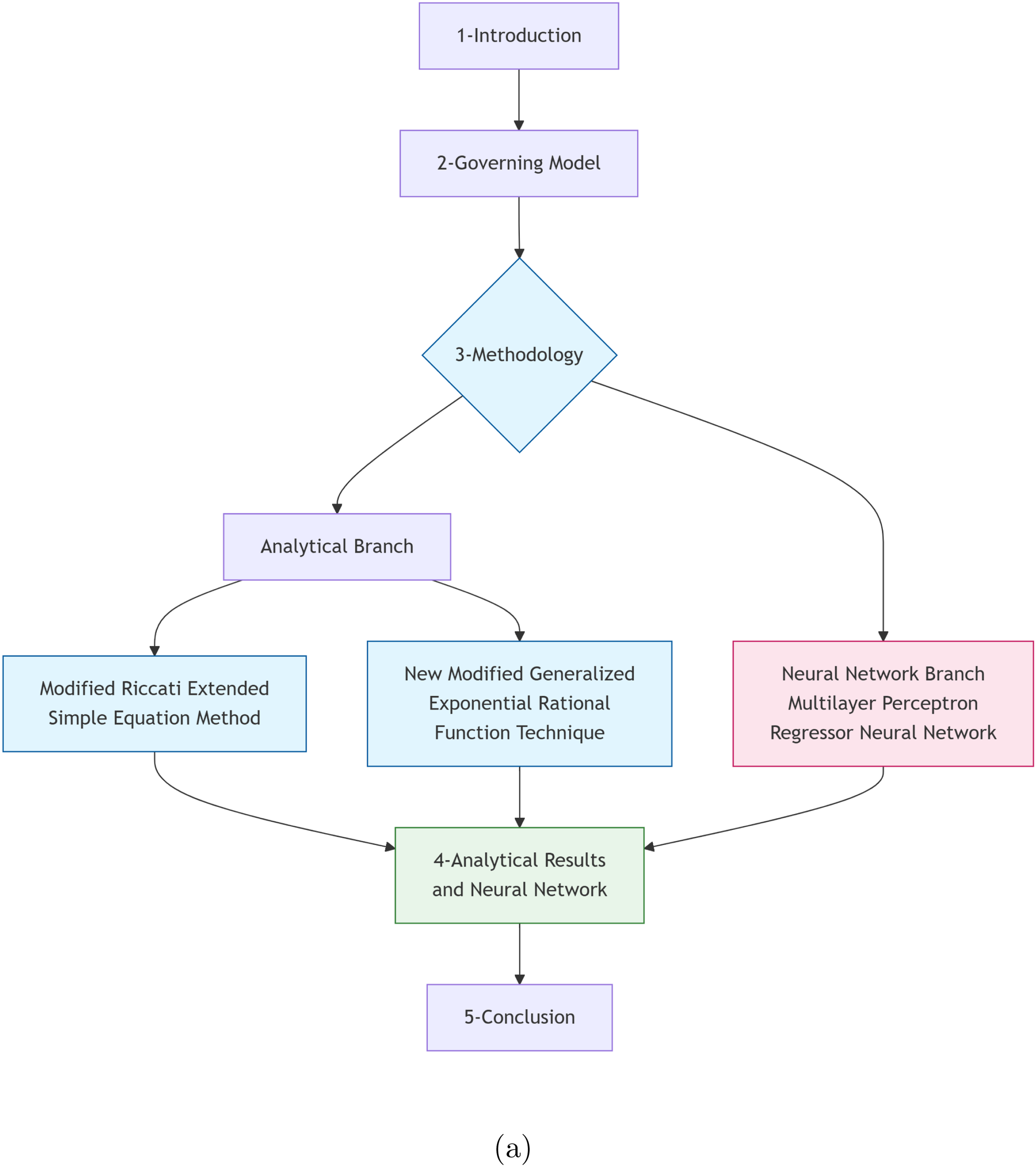

2. The governing equation

The complex Ginzburg-Landau equation is one of the most well-known NLPDE in physics. It describes a wide range of physical phenomena, including nonlinear waves, Bose-Einstein condensation (BEC), second-order phase transitions, superfluidity, superconductivity, liquid crystals, and strings in field theory. To enhance our understanding of nonlinear dynamics, it is beneficial to use mathematical frameworks that elucidate significant concepts across several fields of study. Analytical solutions are required to comprehend the intricate physical effects of nonlinear mathematical problems in nonlinear physics. To study the theory of solitary wave propagation in nonlinear wave dynamics, we need integrable nonlinear models. The complex Ginzburg-Landau equation,^21–24 read as:

$i{W}_t+{\eta }_1{W}_{xx}+{\eta }_2|W{|}^{2}W-\frac{{\eta }_3}{|W{|}^2{W}^{*}}\left(2|W{|}^2{\left(|W{|}^2\right)}_{xx}-{\left({\left(|W{|}^2\right)}_x\right)}^2\right)-{\eta }_{4}W=0,$

(1)

where W = W(x, t) is the complex wave profile with indicated coordinates. In Eq. (1) the parameters η₁, η₂, η₃ and η₄ are represented as: η₁ is the dispersion coefficient that governs the linear dispersive or diffusive behavior of the system. In optical fibers, it corresponds to group velocity dispersion; in plasma, it represents wave spreading due to temperature gradients or density variations. This term balances nonlinearity to facilitate soliton formation. η₂ is the nonlinearity coefficient that represents the dominant nonlinear self-interaction, such as the Kerr effect in optics or ponderomotive nonlinearity in plasma. It is responsible for wave steepening and the formation of bright, dark, or combined solitons depending on its sign relative to dispersion. Besides, the perturbation coefficient is denoted as η₃, which can be used to measure the strength of the higher-order perturbative interactions that will add nonlocal or derivative nonlinearities to the system. Physical phenomena that are explained by this term include self-steepening, Raman scattering, third-order dispersion, or kinetic corrections, and the detuning factor is identified as η₄, and is the frequency detuning or the linear phase mismatch in the system. In optical terms, the phenomenon that is described by the coefficient of η₄ is the angular deviation of the exact resonance of the carrier wave and the natural frequency of the medium. In the plasma physics, it is related to the incompatibility of wave frequency with characteristic plasma frequencies. This parameter is important in the establishment of stability conditions, regimes of existence of solitons, and general energy balance within the system.

Moreover, the proposed model was investigated with the application of various techniques, as in ²¹ trail equation method is applied to describe the soliton solution, where in ²² the new extended direct algebraic method is used to study multiple solitons solution. Also, in ²³ Kumar-Malik and generalized Arnous methods are applied to obtain the soliton solutions of the proposed model, where in ²⁴ modified simple equation method is employed for the investigation of Eq. (1). This study examines the use of novel integration analytical as well as the neural network methods to get diverse soliton solutions and their validation for the specified model.

3. Methodology

Consider

$Q(f,f_t,f_{n_1},f_{n_2},f{f}_{n_1},\cdots )=0.$

(2)

3.1. Modified riccati extended simple equation method

To solve Eq. (2) applying RMSEM, the following procedure will be applied as:

Step-1: A wave hypothesis is introduced and this process changes Eq. (2), into the following ODE:

$R(G,G^{\prime },G{G}^{\prime },\cdots )=0.$

(3)

with G′ = dG/dζ. Then, the balance principle is applied to the Eq. (3) for the further process.

• Step-2: Subsequently, we employ the extended Riccati ODE solution to infer the following series-based solution to the ODE in Eq. (3):

$G(\zeta )=\sum _{j=0}^N{\gamma }_j{\left(\frac{{\mathrm{\Delta }}^{\prime }(\zeta )}{\mathrm{\Delta }(\zeta )}\right)}^j+\sum _{\omega =0}^{N-1}{\chi }_{\omega }{\left(\frac{{\mathrm{\Delta }}^{\prime }(\zeta )}{\mathrm{\Delta }(\zeta )}\right)}^{\omega }\cdot \left(\frac{1}{\mathrm{\Delta }(\zeta )}\right)(\omega =0,1,2,\cdots N-1).$

(4)

The variables γ _j and χ represent the unknown constants that will be determined later. Where, Δ(ζ) denotes the solution of the following Riccati ODE:

${\mathrm{\Delta }}^{\prime }(\zeta )={\beta }_0+{\beta }_1\mathrm{\Delta }(\zeta )+{\beta }_2\mathrm{\Delta }{(\zeta )}^2,$

(5)

where β₀, β₁, β₂ are unknown constants.

• Set-3: The greatest nonlinear component and the highest-order derivative in Eq. (3) can be homogeneously balanced to acquire the positive integer N presented in Eq. (4).

• Step-4: Subsequently, the variables with the same powers of Δ(ζ) are combined when Eq. (4) is substituted into Eq. (3) or the equation that results from the integration of Eq. (3). Expressions in terms of Δ(ζ) are produced during this procedure. A algebraic system of equations containing γ _j and χ _ω , as well as other related parameters, is derived by setting each coefficient in this expression to zero.

• Step-5: The system of nonlinear algebraic equations is analytically evaluated using the Mathematica or Maple tool.

• Step-6: The analytical soliton solutions of Eq. (3) are subsequently obtained by incorporating the derived values of the unknown constants into Eq. (4) along with the Δ(ζ) (the solutions of Eq. (5)). By employing the general solution of Eq. (5), we can generate a variety of soliton solution families as given in 19.

3.2. New modified generalized exponential rational function technique

To obtain the soliton solutions of the presented equation the first step is the same as step 1 in the RMSEM.

Step-2: Consider the solution ²⁰ to Eq. (3):

$\begin{array}{c}\hfill \mathrm{\Phi }(\zeta )={\gamma }_0+\sum _{j=1}^N{\gamma }_j{\left(\mathrm{\Delta }(\zeta )\right)}^j+\sum _{j=1}^N{\beta }_j{\left(\mathrm{\Delta }(\zeta )\right)}^{-j}+\sum _{j=1}^N{\chi }_j{\left(\frac{{\mathrm{\Delta }}^{\prime }(\zeta )}{\mathrm{\Delta }(\zeta )}\right)}^j,\end{array}$

(6)

and

$\mathrm{\Delta }(\zeta )=\frac{{\varsigma }_1{e}^{{\vartheta }_1\zeta }+{\varsigma }_2{e}^{{\vartheta }_2\zeta }}{{\varsigma }_3{e}^{{\vartheta }_3\zeta }+{\varsigma }_4{e}^{{\vartheta }_4\zeta }}.$

(7)

where ς _n and ϑ _n with n = 1, 2, 3, 4 are constants to be extracted.

• Step-3: A polynomial equation is obtained by plugging Eq.(6) into Eq. (3). The polynomial’s coefficients are set to zero, yielding a system of algebraic equations.

• Set-4: The system of equations is solved and the values of γ₀, γ _j , and β _j , χ _j are determined. One may eventually obtain the exact solutions to Eq. (3).

The modified Riccati extended simple equation method and the new modified generalized exponential rational function approach offer distinct advantages over existing analytical techniques. In contrast to the more traditional approaches, e.g. the standard tanh-function method, simplest equation method, simple exp-function method, etc, that provide more limited families of solutions, or use restrictive forms of the ansatz, the modified Riccati extended simple equation method employs the Riccati equation as a scaffolding over which a wider and more diverse base of exact traveling wave solutions, e.g. bright, dark, kink and combined, hyperbolic, periodic and exponential functions solutions, are generated within a more general algebraic framework. Along with this, the new modified generalized exponential rational function method generalizes the classical exponential rational function methods through a more flexible ansatz that allows the discovery of new structures of solutions that are often unreachable through the less general methods discussed. These two methods are especially well adapted to the treatment of higher-order nonlinearities as well as perturbation terms, which most current methods can algebraically treat. Moreover, being algorithmic makes them efficient to implement in symbolic computational systems to reduce the complexity of manual algebraic systems, and guarantee their reproducibility. Together these two approaches constitute a complementary hybrid scheme with the draw the benefit of not only broadening the range of phenomena of exact solitons but also creating a strong foundation of analysis upon which future machine learning applications can be built by offering data of high quality ground truth.

3.3. Multilayer perceptron regressor neural network

The Multi-Layer Perceptron (MLP) regression model which starts by normalizing input features and target values in the range [0,1] and divides the data to 80 percent training and 20 percent testing set that is used in this study. The model architecture is a 2-52-46-1 layer structure with sigmoid, sin and tanh activation functions in the hidden layers and linear activation in the output layer and using Xavier initialize weight initialization and Adam optimizer with 0.1 and 0.01 learning rates to optimize the weights efficiently using gradient. In training on 4000 or more epochs, the model uses forward propagation to make predictions, and mean squared error loss, and back propagation to use gradient descent to update weights, and to periodically report progress. Finally, the trained model makes predictions across the entire spatial-temporal grid and reverses the normalization scaling to produce final results comparable to the original target function values. The model was implemented and trained in Python 3.13.0, using Mean Squared Error (MSE) as the loss function to quantify the disparity between predicted and actual outputs.

4. Extraction of solutions and machine learning validation

Consider the transformation provided by:

$W=W(x,t)=\mathrm{\Phi }(\zeta )e^{i(x-vt)},\zeta =lx-mt;$

(8)

here l, m are real constants. By implementing the transformation in Eq. (1), we get.

$\begin{array}{ccc}\hfill \mathbf{R}\mathbf{e}\mathbf{a}\mathbf{l}\mathbf{P}\mathbf{a}\mathbf{r}\mathbf{t}:\left({\eta }_1{l}^2-4{\eta }_3{l}^2\right){\mathrm{\Phi }}^{″}(\zeta )+{\eta }_2\mathrm{\Phi }{(\zeta )}^3+\mathrm{\Phi }(\zeta )\left(-{\eta }_1-{\eta }_4+v\right)=0,& \hfill & \hfill \end{array}$

(9)

$\begin{array}{ccc}\hfill \mathbf{I}\mathbf{m}\mathbf{a}\mathbf{g}\mathbf{i}\mathbf{n}\mathbf{a}\mathbf{r}\mathbf{y}\mathbf{P}\mathbf{a}\mathbf{r}\mathbf{t}:2{\eta }_{1}l{\mathrm{\Phi }}^{\prime }(\zeta )-m{\mathrm{\Phi }}^{\prime }(\zeta )=0.& \hfill & \hfill \end{array}$

(10)

From imaginary part, we obtain

$m=2l{\eta }_1.$

(11)

Here the real part in Eq. (9) is considered an ODE

$\left({\eta }_1{l}^2-4{\eta }_3{l}^2\right){\mathrm{\Phi }}^{″}(\zeta )+{\eta }_2\mathrm{\Phi }{(\zeta )}^3+\mathrm{\Phi }(\zeta )\left(-{\eta }_1-{\eta }_4+v\right)=0.$

(12)

We find that N = 1 by using the balancing principle in Eq. (12).

4.1. Application of new modified generalized exponential rational function technique

The solution for the nGERFM ²⁰ is represented by

$\begin{array}{c}\hfill \mathrm{\Phi }(\zeta )={\gamma }_0+\sum _{j=1}^N{\gamma }_j{\left(\mathrm{\Delta }(\zeta )\right)}^j+\sum _{j=1}^N{\beta }_j{\left(\mathrm{\Delta }(\zeta )\right)}^{-j}+\sum _{j=1}^N{\chi }_j{\left(\frac{{\mathrm{\Delta }}^{\prime }(\zeta )}{\mathrm{\Delta }(\zeta )}\right)}^j,\end{array}$

(13)

where

$\mathrm{\Delta }(\zeta )=\frac{{\varsigma }_1{e}^{{\vartheta }_1\zeta }+{\varsigma }_2{e}^{{\vartheta }_2\zeta }}{{\varsigma }_3{e}^{{\vartheta }_3\zeta }+{\varsigma }_4{e}^{{\vartheta }_4\zeta }}.$

(14)

When N = 1, Eq. (13) reduces to:

$\mathrm{\Phi }(\zeta )={\gamma }_0+{\gamma }_1\mathrm{\Delta }(\zeta )+{\beta }_1{\left(\mathrm{\Delta }(\zeta )\right)}^{-1}+{\chi }_1\frac{{\mathrm{\Delta }}^{\prime }(\zeta )}{\mathrm{\Delta }(\zeta )}.$

(15)

• • When ς _n = [1, 1, 1, 0] along with ϑ _n = [0, − 1, 0, 0](n = 1, 2, 3, 4), in Eq. (14), results in Δ(ζ) = e^−ζ + 1, while incorporating Eq. (15) into Eq. (12) gives ${\gamma }_1=0,{\beta }_1={\chi }_1-2{\gamma }_0,{\eta }_3=2{\eta }_2{\left({\gamma }_0-{\chi }_1\right)}^2+{\eta }_1{l}^2/4l^2,{\eta }_4={\eta }_2{\left({\gamma }_0-{\chi }_1\right)}^2-{\eta }_1+v$ , then we get:

The exponential solution

$W_1(x,t)=e^{i(x-tv)}\left({\gamma }_0+\frac{{\chi }_1-2{\gamma }_0}{e^{2{\eta }_{1}lt-lx}+1}-\frac{{\chi }_1{e}^{2{\eta }_{1}lt-lx}}{e^{2{\eta }_{1}lt-lx}+1}\right).$

(16)

The explicit hyperbolic solution

$\begin{array}{ccc}\hfill W_2(x,t)=e^{i(x-tv)}\left({\gamma }_0-\frac{2{\gamma }_0}{-\sinh \left(lx-2{\eta }_{1}lt\right)+\cosh \left(lx-2{\eta }_{1}lt\right)+1}+\frac{{\chi }_1}{-\sinh \left(lx-2{\eta }_{1}lt\right)+\cosh \left(lx-2{\eta }_{1}lt\right)+1}\right.& \hfill & \hfill \\ \hfill \left.\frac{{\chi }_1\sinh \left(lx-2{\eta }_{1}lt\right)}{-\sinh \left(lx-2{\eta }_{1}lt\right)+\cosh \left(lx-2{\eta }_{1}lt\right)+1}-\frac{{\chi }_1\cosh \left(lx-2{\eta }_{1}lt\right)}{-\sinh \left(lx-2{\eta }_{1}lt\right)+\cosh \left(lx-2{\eta }_{1}lt\right)+1}\right).& \hfill & \hfill \end{array}$

(17)

• • Next, for ς _n = [2, 0, 1, 1] and ϑ _n = [0, 0, 1, − 1], with Eq. (14), provides that Δ(ζ) = sech(ζ) where employing Eqs. (15) and (12) results in ${\gamma }_0=0,{\gamma }_1=i{\chi }_1,{\beta }_1=0,{\eta }_3=1/4\left({\eta }_1+2{\eta }_2{\chi }_1^2/l^2\right),{\eta }_4={\eta }_2{\chi }_1^2-{\eta }_1+v$ , and ${\gamma }_0=0,{\chi }_1=0,{\beta }_1=0,{\eta }_3={\eta }_1/4-{\gamma }_1^2{\eta }_2/8l^2,{\eta }_4=1/2{\gamma }_1^2{\eta }_2-{\eta }_1+v$ , the following solutions are expressed as follows:

The combined soliton solution

$W_3(x,t)=e^{i(x-tv)}\left(-{\chi }_1\tanh \left(lx-2{\eta }_{1}lt\right)+i{\chi }_1\text{sech}\left(lx-2{\eta }_{1}lt\right)\right),$

(18)

The bright soliton solution

$W_4(x,t)={\gamma }_1{e}^{i(x-tv)}\text{sech}\left(l\left(x-2{\eta }_{1}t\right)\right).$

(19)

• • Taking ς _n = [−i, − i, − i, − i] and ϑ _n = [1, − 1, 0, 0], Eq. (14), offers Δ(ζ) = cosh(ζ), Eqs. (15) and (12) offer η₂ = 0, η₃ = η₁/4, η₄ = v − η₁, gives the soliton solution as:

$W_5(x,t)=e^{-i(tv-x)}\left({\gamma }_0+{\beta }_1\text{sech}\left(l\left(x-2{\eta }_{1}t\right)\right)+{\gamma }_1\cosh \left(l\left(x-2{\eta }_{1}t\right)\right)+{\chi }_1\coth \left(l\left(x-2{\eta }_{1}t\right)\right)\right).$

(20)

• • For the parameters ς _n = [1, 1, 1, 0] and ϑ _n = [3, 2, 0, 0], Eq. (14), transforms to Δ(ζ) = e^3ζ + e^2ζ, where putting Eq. (15) in (12) gives ${\gamma }_0=-1/2\left(5{\chi }_1\right),{\gamma }_1=0,{\beta }_1=0,{\eta }_3=1/8\left(2{\eta }_1+{\eta }_2{\chi }_1^2/l^2\right),{\eta }_4=1/4{\eta }_2{\chi }_1^2-{\eta }_1+v$ , then we get:

$W_6(x,t)=e^{i(x-tv)}\left(\frac{{\chi }_1\left(2e^{2\left(lx-2{\eta }_{1}lt\right)}+3e^{3\left(lx-2{\eta }_{1}lt\right)}\right)}{e^{2\left(lx-2{\eta }_{1}lt\right)}+e^{3\left(lx-2{\eta }_{1}lt\right)}}-\frac{5{\chi }_1}{2}\right).$

(21)

Where, its hyperbolic form solution

$\begin{array}{ccc}\hfill W_7(x,t)=e^{i(x-tv)}& \hfill & \hfill \\ \hfill \left(\frac{{\chi }_1\left(2\sinh \left(2\left(lx-2{\eta }_{1}lt\right)\right)+3\sinh \left(3\left(lx-2{\eta }_{1}lt\right)\right)+2\cosh \left(2\left(lx-2{\eta }_{1}lt\right)\right)+3\cosh \left(3\left(lx-2{\eta }_{1}lt\right)\right)\right)}{\sinh \left(2\left(lx-2{\eta }_{1}lt\right)\right)+\sinh \left(3\left(lx-2{\eta }_{1}lt\right)\right)+\cosh \left(2\left(lx-2{\eta }_{1}lt\right)\right)+\cosh \left(3\left(lx-2{\eta }_{1}lt\right)\right)}-\frac{5{\chi }_1}{2}\right).& \hfill & \hfill \end{array}$

(22)

• • Choosing ς _n = [1, − 1, 2, 0] and ϑ _n = [2, 0, 0, 0], then Eq. (14), provides Δ(ζ) = e ^ζ sinh(ζ), Eqs. (15) along with (12) results in ${\gamma }_1=0,{\beta }_1={\gamma }_0+{\chi }_1,{\eta }_3={\eta }_2\left({\gamma }_0+2{\chi }_1\right){}^2+2{\eta }_1{l}^2/8l^2,{\eta }_4={\eta }_2\left({\gamma }_0+2{\chi }_1\right){}^2-{\eta }_1+v$ , we get:

$W_8(x,t)=e^{i(x-tv)}\left({\gamma }_0+\left({\gamma }_0+{\chi }_1\right)e^{2{\eta }_{1}lt-lx}\text{csch}\left(lx-2{\eta }_{1}lt\right)+{\chi }_1{e}^{lx-2{\eta }_{1}lt}\text{csch}\left(lx-2{\eta }_{1}lt\right)\right).$

(23)

• • Similarly, for ς _n = [1, 1, 2, 0] and ϑ _n = [i, − i, 0, 0](n = 1, 2, 3, 4), Eq. (14), implies that Δ(ζ) = cos ζ, Eqs. (15) and (12) provide ${\gamma }_0=0,{\gamma }_1=0,{\beta }_1=-{\chi }_1,{\eta }_3=1/4\left({\eta }_1+2{\eta }_2{\chi }_1^2/l^2\right),{\eta }_4=-{\eta }_2{\chi }_1^2-{\eta }_1+v$ , and ${\gamma }_0=0,{\gamma }_1=0,{\chi }_1=0,{\eta }_3=1/8\left(2{\eta }_1+{\beta }_1^2{\eta }_2/l^2\right),{\eta }_4=1/2{\beta }_1^2{\eta }_2-{\eta }_1+v$ , we get:

$W_9(x,t)=e^{i(x-tv)}\left({\chi }_1\left(-\sec \left(lx-2{\eta }_{1}lt\right)\right)-{\chi }_1\tan \left(lx-2{\eta }_{1}lt\right)\right),$

(24)

$W_{10}(x,t)={\beta }_1{e}^{i(x-tv)}\sec \left(lx-2{\eta }_{1}lt\right).$

(25)

• • Choosing ς _n = [1, − 1, i, i] and ϑ _n = [i, − i, 0, 0], then Eq. (14), gives Δ(ζ) = sin ζ, Eqs. (15) and (12) provide ${\gamma }_0=0,{\gamma }_1=0,{\beta }_1=-{\chi }_1,{\eta }_3=1/4\left({\eta }_1+2{\eta }_2{\chi }_1^2/l^2\right),{\eta }_4=-{\eta }_2{\chi }_1^2-{\eta }_1+v$ , and ${\gamma }_0=0,{\gamma }_1=0,{\chi }_1=0,{\eta }_3=1/8\left(2{\eta }_1+{\beta }_1^2{\eta }_2/l^2\right),{\eta }_4=1/2{\beta }_1^2{\eta }_2-{\eta }_1+v$ , we get:

$W_{11}(x,t)=e^{i(x-tv)}\left({\chi }_1\cot \left(lx-2{\eta }_{1}lt\right)-{\chi }_1\csc \left(lx-2{\eta }_{1}lt\right)\right),$

(26)

$W_{12}(x,t)={\beta }_1{e}^{i(x-tv)}\csc \left(l\left(x-2{\eta }_{1}t\right)\right).$

(27)

• • Data-driven solutions of Eq. (16)

In this case, our aim is to check the performance of the soliton solution mentioned obtained in Eq. (16). The model architecture consisted of two hidden layers and a sin activation function. The Adam optimizer was used with a learning rate of 0.01 and 1500 training epochs.

In the Figure 2 the subplot (a) show thes exact dynamics and subplot (b) represents predicted dynamics and error in the subplot (c), the combined dynamics is represented in subplot (d) for the real dynamics of the solution (16) for the parametric values v = .01, γ₀ = 1.52, l = .056, η₁ = .09, χ₁ = .52. The graph shows the training loss for each epoch in subplot (e).

Figure 2.

Plots for the real dynamics of the solution (16).

The corresponding, epoch-wise loss values is mentioned as:

The exact and predicted behaviour of solution (16) at the different values of the t have been discussed in the Figure 3.

Figure 3.

Graphs for the real dynamics to the solution (16).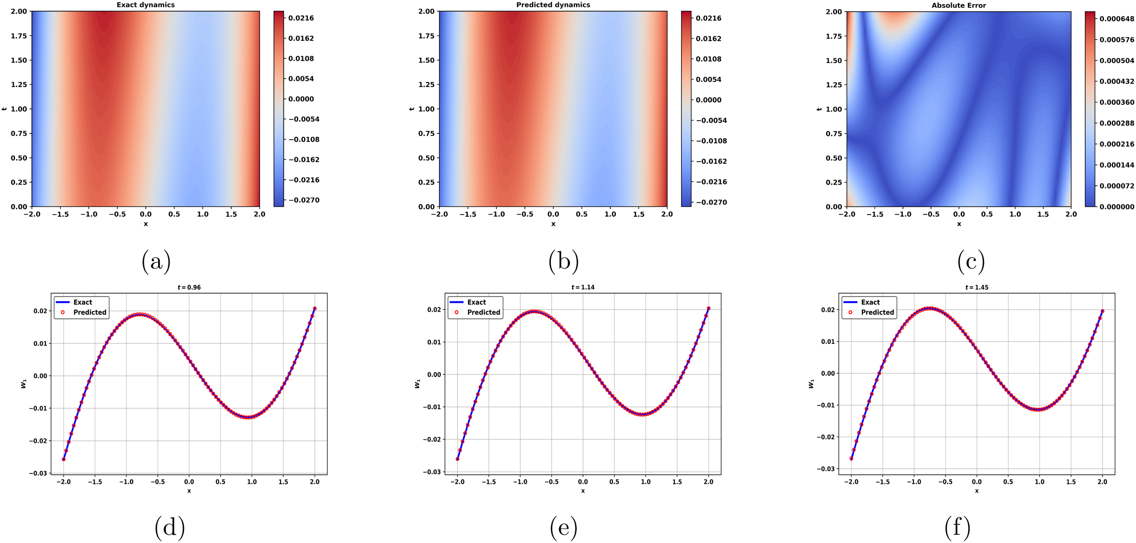

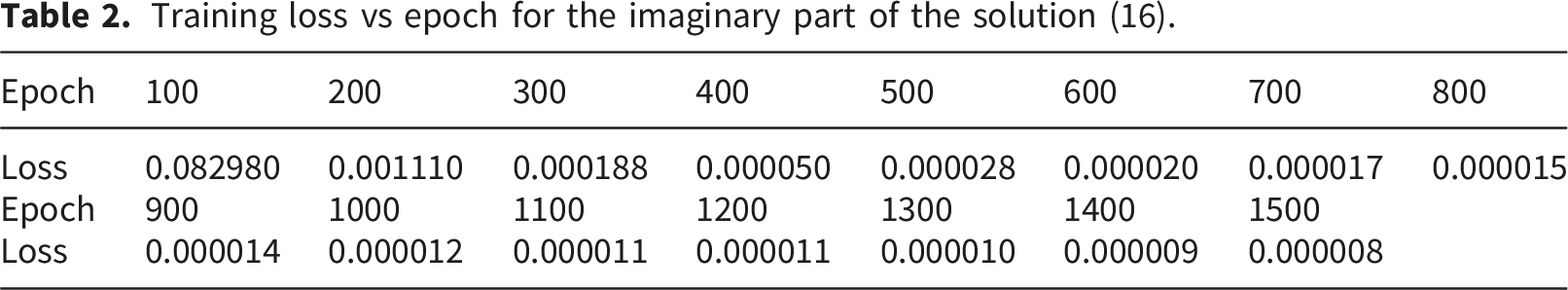
Moreover, the imaginary behaviour of the solution (16) with the parametric values v = .01, γ₀ = 1.52, l = 0.056, η₁ = .09, χ₁ = .52 has been discussed and performance of the solution have been checked. Figure 4 contains five subplots: (a) exact dynamics, (b) predicted dynamics, (c) absolute error, (d) combined exact-predicted dynamics, and (e) training loss by epoch. The epoch-wise loss is mentioned as:

Figure 4.

Graphs for the imaginary dynamics to the solution (16).

The exact and predicted behaviour of solution (16) at the different values of the t have been discussed in the Figure 5. The above figures illustrate the propagation of the combined and dark soliton solutions. Dark solitons fiber are applied to transmit data in a stable way using dark pulses. They model topological defects and quantum vortices in Bose-Einstein Condensates. Their properties are key for studying nonlinear waves in superfluids and plasmas. They also act as information carriers in developing photonic logic circuits. Moreover, the performance of activation function suggests it should be the preferred choice for similar problems involving nonlinear solutions.

• Data-driven solutions of Eq. (19)

Figure 5.

Graphs for the imaginary dynamics to the solution (16).

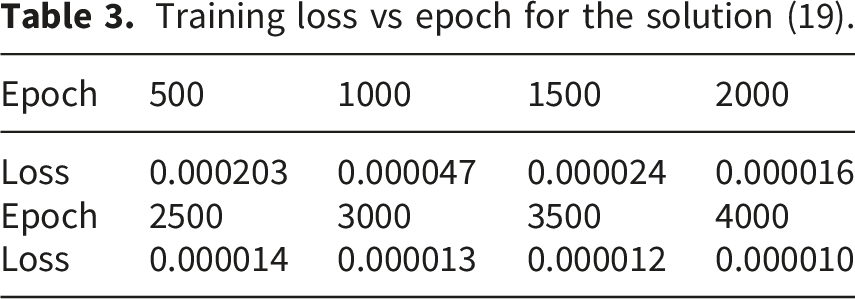
The performance of the absolute behaviour of the solution (19) has been explored with the learning rate 0.1 and sigmoid activation function. The model was trained upto 4000 training epochs. The exact, predicted, combined dynamics and the training loss corresponding to the each epoch for the solution Eq. (19) for the v = 0.01, l = 1.2, η₁ = 0.19, γ₁ = 0.22 are mentioned in Figure 6 as:

Figure 6.

Graphs for the absolute behaviour to the solution (19).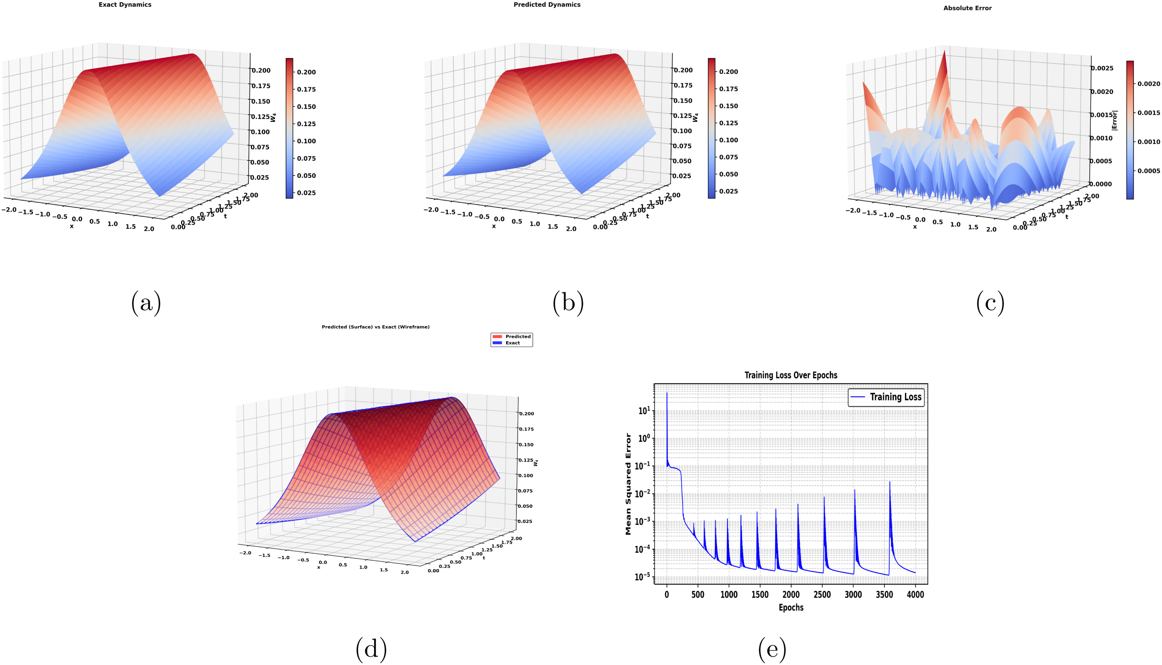

The corresponding, epoch-wise loss values is mentioned as:

The exact and predicted behaviour of solution (19) at the different values of the t have been discussed in the Figure 7. The 3 dimensional, contour and two dimensional graphs show the dynamics of the bright soliton. The plots vividly demonstrate the bright soliton’s stable, particle like propagation maintaining its shape and amplitude over distance a crucial property for optical communication. Moreover, the bright solitons enable ultra-long distance, high-speed data transmission in optical fibers by perfectly balancing nonlinear and dispersive effects, revolutionizing modern telecommunications infrastructure.

Figure 7.

Graphs for the absolute dynamics to the solution (19).

4.2. Application of modified riccati extended simple equation technique

Consider the ¹⁹ as:

$\mathrm{\Phi }(\zeta )=\sum _{j=0}^N{\gamma }_j{\left(\frac{{\mathrm{\Delta }}^{\prime }(\zeta )}{\mathrm{\Delta }(\zeta )}\right)}^j+\sum _{\omega =0}^{N-1}{\chi }_{\omega }{\left(\frac{{\mathrm{\Delta }}^{\prime }(\zeta )}{\mathrm{\Delta }(\zeta )}\right)}^{\omega }\cdot \left(\frac{1}{\mathrm{\Delta }(\zeta )}\right)(\omega =0,1,2,\cdots N-1).$

(28)

Taking N = 1, in Eq. (28) results in

$\mathrm{\Phi }(\zeta )={\gamma }_0+{\gamma }_1\left(\frac{{\mathrm{\Delta }}^{\prime }(\zeta )}{\mathrm{\Delta }(\zeta )}\right)+\frac{{\chi }_0}{\mathrm{\Delta }(\zeta )},$

(29)

with Δ′(ζ) = β₀ + β₁Δ(ζ) + β₂Δ(ζ)².

The incorporation of Eq. (28) and Eq. (29) into Eq. (12) produces the solutions as:

Family-1:

• Set-1: For ${\gamma }_0=-1/2{\beta }_1{\gamma }_1,{\chi }_0=-{\beta }_0{\gamma }_1,{\eta }_3=1/8\left(2{\eta }_1+{\gamma }_1^2{\eta }_2/l^2\right),{\eta }_4=-{\eta }_1+v+1/4{\gamma }_1^2{\eta }_2\mathcal{H},\mathcal{H}={\beta }_1^2-4{\beta }_0{\beta }_2<0$ , we obtain the periodic solution as:

$W_1(x,t)=e^{i(x-tv)}\left(-\frac{1}{2}{\beta }_1{\gamma }_1-\frac{{\gamma }_1\mathcal{H}\left({\tan }^2\left(\frac{1}{2}\sqrt{-\mathcal{H}}(lx-mt)\right)+1\right)}{2\left(\sqrt{-\mathcal{H}}\tan \left(\frac{1}{2}\sqrt{-\mathcal{H}}(lx-mt)\right)-{\beta }_1\right)}-\frac{{\beta }_0{\gamma }_1}{\frac{\sqrt{-\mathcal{H}}\tan \left(\frac{1}{2}\sqrt{-\mathcal{H}}(lx-mt)\right)}{2{\beta }_2}-\frac{{\beta }_1}{2{\beta }_2}}\right).$

(30)

• • Set-2: When ${\gamma }_1=0,{\chi }_0=2{\beta }_0{\gamma }_0/{\beta }_1,{\eta }_3=1/4\left({\eta }_1+2{\gamma }_0^2{\eta }_2/{\beta }_1^2{l}^2\right),{\eta }_4=\left(1-4{\beta }_0{\beta }_2/{\beta }_1^2\right){\gamma }_0^2{\eta }_2-{\eta }_1+v,\mathcal{H}={\beta }_1^2-4{\beta }_0{\beta }_2<0$ , gives the periodic solution such as:

$W_2(x,t)={\gamma }_0{e}^{i(x-tv)}\left(1-\frac{4{\beta }_0{\beta }_2}{{\beta }_1^2-{\beta }_1\sqrt{-\mathcal{H}}\tan \left(\frac{1}{2}\sqrt{-\mathcal{H}}(lx-mt)\right)}\right).$

(31)

Family-2:

• Set-1: When ${\gamma }_0=-1/2{\beta }_1{\gamma }_1,{\chi }_0=-{\beta }_0{\gamma }_1,{\eta }_3=1/8\left(2{\eta }_1+{\gamma }_1^2{\eta }_2/l^2\right),{\eta }_4=-{\eta }_1+v+1/4{\gamma }_1^2{\eta }_2\mathcal{H},\mathcal{H}={\beta }_1^2-4{\beta }_0{\beta }_2<0$ , the soliton solution is obtained as:

$W_3(x,t)=\frac{{\gamma }_1{e}^{ix-itv}\cot \left(\frac{1}{2}\sqrt{-\mathcal{H}}(lx-mt)\right)\left({\beta }_1^2\cot \left(\frac{1}{2}\sqrt{-\mathcal{H}}(lx-mt)\right)-4{\beta }_0{\beta }_2\cot \left(\frac{1}{2}\sqrt{-\mathcal{H}}(lx-mt)\right)-{\beta }_1\sqrt{-\mathcal{H}}\right)}{2\left({\beta }_1+\sqrt{-\mathcal{H}}\cot \left(\frac{1}{2}\sqrt{-\mathcal{H}}(lx-mt)\right)\right)}.$

(32)

• • Set-2: When ${\gamma }_1=0,{\chi }_0=2{\beta }_0{\gamma }_0/{\beta }_1,{\eta }_3=1/4\left({\eta }_1+2{\gamma }_0^2{\eta }_2/{\beta }_1^2{l}^2\right),{\eta }_4=\left(1-4{\beta }_0{\beta }_2/{\beta }_1^2\right){\gamma }_0^2{\eta }_2-{\eta }_1+v,\mathcal{H}={\beta }_1^2-4{\beta }_0{\beta }_2<0$ , we have:

$W_4(x,t)={\gamma }_0{e}^{i(x-tv)}\left(1-\frac{4{\beta }_0{\beta }_2}{{\beta }_1^2+{\beta }_1\sqrt{-\mathcal{H}}\cot \left(\frac{1}{2}\sqrt{-\mathcal{H}}(lx-mt)\right)}\right).$

(33)

Family-3:

• Set-1: When ${\gamma }_0=-1/2{\beta }_1{\gamma }_1,{\chi }_0=-{\beta }_0{\gamma }_1,{\eta }_3=1/8\left(2{\eta }_1+{\gamma }_1^2{\eta }_2/l^2\right),{\eta }_4=-{\eta }_1+v+1/4{\gamma }_1^2{\eta }_2\mathcal{H},\mathcal{H}={\beta }_1^2-4{\beta }_0{\beta }_2<0$ , then

$\begin{array}{ccc}\hfill W_5(x,t)=e^{i(x-tv)}\left(\frac{{\gamma }_1(-\mathcal{H})\left(\sin \left(\sqrt{-\mathcal{H}}(lx-mt)\right)+1\right)\sec \left(\sqrt{-\mathcal{H}}(lx-mt)\right)}{-{\beta }_1\cos \left(\sqrt{-\mathcal{H}}(lx-mt)\right)+\sqrt{-\mathcal{H}}\sin \left(\sqrt{-\mathcal{H}}(lx-mt)\right)+\sqrt{-\mathcal{H}}}-\frac{{\beta }_1{\gamma }_1}{2}\right.& \hfill & \hfill \\ \hfill \left.-\frac{{\beta }_0{\gamma }_1}{\frac{\sqrt{-\mathcal{H}}\left(\tan \left(\sqrt{-\mathcal{H}}(lx-mt)\right)+\sec \left(\sqrt{-\mathcal{H}}(lx-mt)\right)\right)}{2{\beta }_2}-\frac{{\beta }_1}{2{\beta }_2}}\right).& \hfill & \hfill \end{array}$

(34)

• • Set-2: When ${\gamma }_1=0,{\chi }_0=2{\beta }_0{\gamma }_0/{\beta }_1,{\eta }_3=1/4\left({\eta }_1+2{\gamma }_0^2{\eta }_2/{\beta }_1^2{l}^2\right),{\eta }_4=\left(1-4{\beta }_0{\beta }_2/{\beta }_1^2\right){\gamma }_0^2{\eta }_2-{\eta }_1+v,\mathcal{H}={\beta }_1^2-4{\beta }_0{\beta }_2<0$ , results in the periodic solution as follows:

$W_6(x,t)={\gamma }_0{e}^{i(x-tv)}\left(1-\frac{4{\beta }_0{\beta }_2}{{\beta }_1\left({\beta }_1-\sqrt{-\mathcal{H}}\left(\tan \left(\sqrt{-\mathcal{H}}(lx-mt)\right)+\sec \left(\sqrt{-\mathcal{H}}(lx-mt)\right)\right)\right)}\right).$

(35)

Family-4:

When ${\gamma }_0=-1/2{\beta }_1{\gamma }_1,{\chi }_0=-{\beta }_0{\gamma }_1,{\eta }_3=1/8\left(2{\eta }_1+{\gamma }_1^2{\eta }_2/l^2\right),{\eta }_4=-{\eta }_1+v+1/4{\gamma }_1^2{\eta }_2\mathcal{H},\mathcal{H}={\beta }_1^2-4{\beta }_0{\beta }_2>0$ , we have

$W_7(x,t)=e^{i(x-tv)}\left(-\frac{1}{2}{\beta }_1{\gamma }_1-\frac{{\gamma }_1\mathcal{H}\left({\tanh }^2\left(\frac{1}{2}\sqrt{\mathcal{H}}(lx-mt)\right)-1\right)}{2\left({\beta }_1+\sqrt{\mathcal{H}}\tanh \left(\frac{1}{2}\sqrt{\mathcal{H}}(lx-mt)\right)\right)}-\frac{{\beta }_0{\gamma }_1}{-\frac{{\beta }_1}{2{\beta }_2}-\frac{\sqrt{\mathcal{H}}\tanh \left(\frac{1}{2}\sqrt{\mathcal{H}}(lx-mt)\right)}{2{\beta }_2}}\right).$

(36)

• • Set-2: When ${\gamma }_1=0,{\chi }_0=2{\beta }_0{\gamma }_0/{\beta }_1,{\eta }_3=1/4\left({\eta }_1+2{\gamma }_0^2{\eta }_2/{\beta }_1^2{l}^2\right),{\eta }_4=\left(1-4{\beta }_0{\beta }_2/{\beta }_1^2\right){\gamma }_0^2{\eta }_2-{\eta }_1+v,\mathcal{H}={\beta }_1^2-4{\beta }_0{\beta }_2>0$ , we have:

$W_8(x,t)={\gamma }_0{e}^{i(x-tv)}\left(1-\frac{4{\beta }_0{\beta }_2}{{\beta }_1^2+{\beta }_1\sqrt{\mathcal{H}}\tanh \left(\frac{1}{2}\sqrt{\mathcal{H}}(lx-mt)\right)}\right).$

(37)

• • Data-driven solutions of Eq. (37)

The soliton solution (37) is under consideration for applying the neural networking technique. For this, we have selected the tanh as the activation function with the learning rate 0.01 and the training upto 2000 epochs.

In the Figure 8 the different subplots are discussed for the real dynamics of the solution (37) with the parametric values m = 0.1, v = 0.01, γ₀ = 0.1, l = .39, β₁ = 2.04, β₀ = 0.4, β₂ = 1.1.

Figure 8.

Plots for the real dynamics of the solution (37).

The corresponding, epoch-wise loss values is mentioned as:

The exact and predicted behaviour in the density plots and two dimensional graphs in the blue line represents the actual data and red circles show the predict data behavior of solution (37) at the different values of the t have been discussed in the Figure 9.

Figure 9.

Plots for the real dynamics of the solution (37).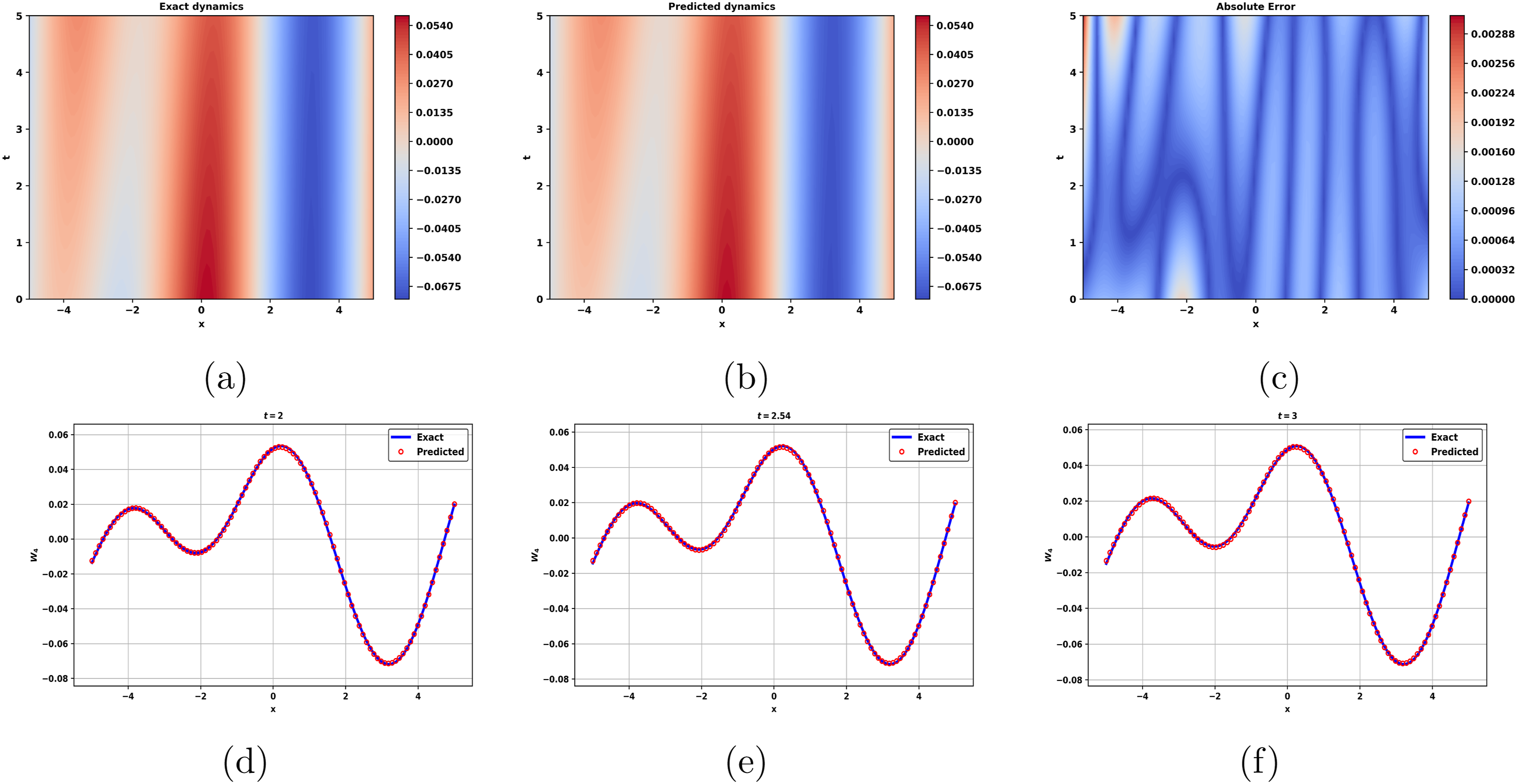

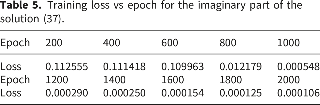
Further more, the performance of the imaginary part of the solution the (37) is discussed with parametric values m = 0.1, v = 2.01, γ₀ = 0.1, l = 0.1, β₁ = 1.04, β₀ = .4, β₂ = .1. The tanh is considered as the activation function with the training upto 2000 epochs and learning rate is 0.01. The different aspects are offered in the Figure 10. The corresponding, epoch-wise loss values is mentioned as:(Figure 11)

Figure 10.

Graphs for the solution for the imaginary dynamics to the solution (37).

Figure 11.

Graphs for the imaginary dynamics to the solution (37). The exact and predicted behaviour in the density plots and two dimensional graphs at the different values of the t.

Family-5:

• Set-1: When ${\gamma }_0=-1/2{\beta }_1{\gamma }_1,{\chi }_0=-{\beta }_0{\gamma }_1,{\eta }_3=1/8\left(2{\eta }_1+{\gamma }_1^2{\eta }_2/l^2\right),{\eta }_4=-{\eta }_1+v+1/4{\gamma }_1^2{\eta }_2\mathcal{H},\mathcal{H}={\beta }_1^2-4{\beta }_0{\beta }_2>0$ , we obtain the dark soliton solution:

$\begin{array}{ccc}\hfill W_9(x,t)=e^{i(x-tv)}\left(-\frac{1}{2}{\beta }_1{\gamma }_1-\frac{{\gamma }_1\mathcal{H}\left(-1+i\sinh \left(\sqrt{\mathcal{H}}(lx-mt)\right)\right)\text{sech}\left(\sqrt{\mathcal{H}}(lx-mt)\right)}{{\beta }_1\cosh \left(\sqrt{\mathcal{H}}(lx-mt)\right)+\sqrt{\mathcal{H}}\sinh \left(\sqrt{\mathcal{H}}(lx-mt)\right)+i\sqrt{\mathcal{H}}}\right.& \hfill & \hfill \\ \hfill \left.-\frac{{\beta }_0{\gamma }_1}{-\frac{{\beta }_1}{2{\beta }_2}-\frac{\sqrt{\mathcal{H}}\left(\tanh \left(\sqrt{\mathcal{H}}(lx-mt)\right)+i\text{sech}\left(\sqrt{\mathcal{H}}(lx-mt)\right)\right)}{2{\beta }_2}}\right).& \hfill & \hfill \end{array}$

(38)

• • Set-2: When ${\gamma }_1=0,{\chi }_0=2{\beta }_0{\gamma }_0/{\beta }_1,{\eta }_3=1/4\left({\eta }_1+2{\gamma }_0^2{\eta }_2/{\beta }_1^2{l}^2\right),{\eta }_4=\left(1-4{\beta }_0{\beta }_2/{\beta }_1^2\right){\gamma }_0^2{\eta }_2-{\eta }_1+v,\mathcal{H}={\beta }_1^2-4{\beta }_0{\beta }_2>0$ , we obtain:

$W_{10}(x,t)={\gamma }_0{e}^{i(x-tv)}\left(1-\frac{4{\beta }_0{\beta }_2}{{\beta }_1\left({\beta }_1+\sqrt{\mathcal{H}}\left(\tanh \left(\sqrt{\mathcal{H}}(lx-mt)\right)+i\text{sech}\left(\sqrt{\mathcal{H}}(lx-mt)\right)\right)\right)}\right).$

(39)

Family-6:

When ${\gamma }_0=-1/2{\beta }_1{\gamma }_1,{\chi }_0=-{\beta }_0{\gamma }_1,{\eta }_3=1/8\left(2{\eta }_1+{\gamma }_1^2{\eta }_2/l^2\right),{\eta }_4=-{\eta }_1+v+1/4{\gamma }_1^2{\eta }_2\mathcal{H},\mathcal{H}={\beta }_1^2-4{\beta }_0{\beta }_2>0$ , we get the solution:

$\begin{array}{ccc}\hfill W_{11}(x,t)=e^{i(x-tv)}\left(-\frac{1}{2}{\beta }_1{\gamma }_1-\frac{{\gamma }_1\mathcal{H}\left(1+i\sinh \left(\sqrt{\mathcal{H}}(lx-mt)\right)\right)\text{sech}\left(\sqrt{\mathcal{H}}(lx-mt)\right)}{-{\beta }_1\cosh \left(\sqrt{\mathcal{H}}(lx-mt)\right)-\sqrt{\mathcal{H}}\sinh \left(\sqrt{\mathcal{H}}(lx-mt)\right)+i\sqrt{\mathcal{H}}}\right.& \hfill & \hfill \\ \hfill \left.-\frac{{\beta }_0{\gamma }_1}{-\frac{{\beta }_1}{2{\beta }_2}-\frac{\sqrt{\mathcal{H}}\left(\tanh \left(\sqrt{\mathcal{H}}(lx-mt)\right)-i\text{sech}\left(\sqrt{\mathcal{H}}(lx-mt)\right)\right)}{2{\beta }_2}}\right).& \hfill & \hfill \end{array}$

(40)

Family-7:

When ${\gamma }_1=0;{\chi }_0=2{\beta }_0{\gamma }_0/{\beta }_1;{\eta }_3=1/4\left({\eta }_1+2{\gamma }_0^2{\eta }_2/{\beta }_1^2{l}^2\right);{\eta }_4=\left(1-4{\beta }_0{\beta }_2/{\beta }_1^2\right){\gamma }_0^2{\eta }_2-{\eta }_1+v;\mathcal{H}={\beta }_1^2-4{\beta }_0{\beta }_2>0$ , we have

$W_{12}(x,t)={\gamma }_0{e}^{i(x-tv)}\left(1-\frac{4{\beta }_0{\beta }_2}{{\beta }_1^2+{\beta }_1\sqrt{\mathcal{H}}\coth \left(\frac{1}{2}\sqrt{\mathcal{H}}(lx-mt)\right)}\right).$

(41)

Family-8:

When ${\gamma }_1=0,{\chi }_0=2{\beta }_0{\gamma }_0/{\beta }_1,{\eta }_3=1/4\left({\eta }_1+2{\gamma }_0^2{\eta }_2/{\beta }_1^2{l}^2\right),{\eta }_4={\gamma }_0^2{\eta }_2-{\eta }_1+v,{\beta }_2=0,{\beta }_1=\tau ,{\beta }_0=h\tau$ , we get the following soliton solution:

$W_{13}(x,t)={\gamma }_0{e}^{i(x-tv)}\left(\frac{2h}{e^{l\tau x-mt\tau }-h}+1\right).$

(42)

• Data-driven solutions of Eq. (42)

The machine learning validation has been discussed for the absolute behaviour of the solution (44) by applying the sigmoid activation function. The model has been trained upto 2800 epochs with the learning rate 0.01. The exact, predicted, combined dynamics and the training loss corresponding to the each epoch to the solution Eq. (42) for the m = 0.023v = 1.8, γ₀ = 0.1, τ = 0.1, h = 2.225, l = 1.34 are mentioned in Figure 12 as:

Figure 12.

Graphs for the absolute behaviour to the solution (42).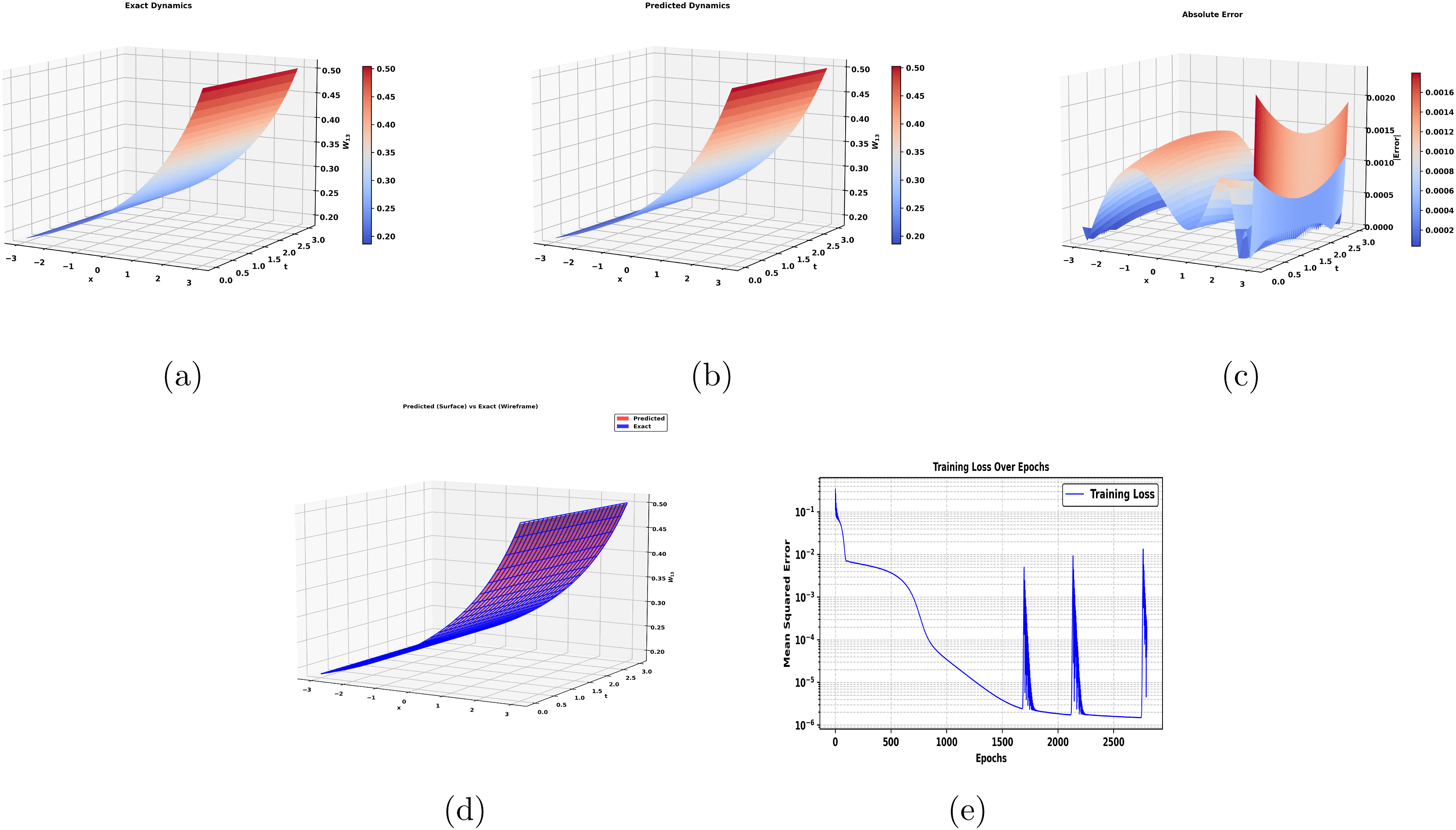

The exact and predicted behaviour in the density plots and two dimensional graphs in the blue line represents the actual data and red circles show the predict data behavior of solution (42) at the different values of the t(Figure 13).

Figure 13.

Plots for the absolute dynamics of the solution (42).

The corresponding, epoch-wise loss values is mentioned as:

Family-9:

When ${\gamma }_0=-1/2{\beta }_1{\gamma }_1,{\chi }_0=0,{\eta }_3=1/8\left(2{\eta }_1+{\gamma }_1^2{\eta }_2/l^2\right),{\eta }_4=1/4{\beta }_1^2{\gamma }_1^2{\eta }_2-{\eta }_1+v,{\beta }_0=0,{\beta }_1=\tau ,{\beta }_2=h\tau$ , we get:

$W_{14}(x,t)=\frac{1}{2}{\gamma }_1\tau e^{i(x-tv)}\left(-\frac{2}{h{e}^{l\tau x-mt\tau }-1}-1\right).$

(43)

Family-10:

When ${\gamma }_0=-1/2{\beta }_1{\gamma }_1,{\chi }_0=0,{\eta }_3=1/8\left(2{\eta }_1+{\gamma }_1^2{\eta }_2/l^2\right),{\eta }_4=1/4{\beta }_1^2{\gamma }_1^2{\eta }_2-{\eta }_1+v,{\beta }_0=0$ , the soliton solution we get is as follows:

$W_{15}(x,t)=e^{i(x-tv)}\left(\frac{{\beta }_1{\gamma }_1\left(\sinh \left({\beta }_1(lx-mt)\right)-\cosh \left({\beta }_1(lx-mt)\right)\right)}{\sinh \left({\beta }_1(lx-mt)\right)-\cosh \left({\beta }_1(lx-mt)\right)-\omega }-\frac{{\beta }_1{\gamma }_1}{2}\right).$

(44)

5. Conclusion

This paper has widely explored the the complex Ginzburg-Landau equation with several aspects. In the first phase, the soliton solutions have been developed by introducing the traveling wave transformation and getting the corresponding ordinary differential equation. Then, the comprehensive analytical methods, including the nGERFM, and RMSEM were applied to the ordinary differential equation based on the balance principle that is N = 1. The solutions like dark, periodic, bright, hyperbolic, combined, and exponential soliton solutions were secured with different parameters. Thus, in the second phase of this study, the neural network has been applied to check the performance and validation of the obtained solutions. The results have been discussed in the Figures 2–11, Figure 12, Figure 13, also the training epochs and corresponding loss values for the discussed solutions were discussed in the Tables 1–6. The analytical techniques and machine learning synergy create an all-inclusive and adaptive and robust structure of solving a nonlinear evolution equation. It simultaneously provides both symbolic methods of correctly finding the precise soliton solutions and data-driven discovery and simulation by neural networks, providing a scalable and reproducible route to the modeling of the complex wave phenomenon. The usefulness of the work in practice spans a wide range of physical systems such as plasma physics, fiber optics and condensate dynamics that offers a general guide on future research studying more demanding systems such as higher-dimensional wave fields, nonlocal interactions, and perturbed nonlinear models. The present study provides a blueprint of the future generations of hybrid scientific computing structures by showing that classical analysis and modern learning architectures can be mutually reinforcing.

Table 1.

Training loss vs epoch for the real part of the solution (16).

Epoch	100	200	300	400	500	600	700	800
Loss	0.053272	0.053234	0.053134	0.051988	0.000369	0.000114	0.000062	0.000039
Epoch	900	1000	1100	1200	1300	1400	1500	​
Loss	0.000026	0.000019	0.000014	0.000011	0.000009	0.000007	0.000006	​

Table 2.

Training loss vs epoch for the imaginary part of the solution (16).

Epoch	100	200	300	400	500	600	700	800
Loss	0.082980	0.001110	0.000188	0.000050	0.000028	0.000020	0.000017	0.000015
Epoch	900	1000	1100	1200	1300	1400	1500	​
Loss	0.000014	0.000012	0.000011	0.000011	0.000010	0.000009	0.000008	​

Table 3.

Training loss vs epoch for the solution (19).

Epoch	500	1000	1500	2000
Loss	0.000203	0.000047	0.000024	0.000016
Epoch	2500	3000	3500	4000
Loss	0.000014	0.000013	0.000012	0.000010

Table 4.

Training loss vs epoch for the real part of the solution (37).

Epoch	100	400	600	800	1000
Loss	0.053913	0.038763	0.001204	0.000566	0.000315
Epoch	1200	1400	1600	1800	2000
Loss	0.000155	0.000084	0.000044	000040	0.000020

Table 5.

Training loss vs epoch for the imaginary part of the solution (37).

Epoch	200	400	600	800	1000
Loss	0.112555	0.111418	0.109963	0.012179	0.000548
Epoch	1200	1400	1600	1800	2000
Loss	0.000290	0.000250	0.000154	0.000125	0.000106

Table 6.

Training loss vs epoch for the solution (42).

Epoch	200	400	600	800	1000	1200	1400
Loss	0.006179	0.004704	0.002456	0.000170	0.000035	0.000014	0.000006
Epoch	1600	1800	2000	2200	2400	2600	2800
Loss	0.000004	0.000004	0.000003	0.000003	0.000002	0.000002	0.000001