Sage Journals: Discover world-class research

Abstract

In this paper, a neural network model combining wavelet decomposition and attention mechanism is proposed for the accurate prediction of non-stationary wind pressure on the surface of the glass curtain wall of an airport terminal building under strong wind conditions. The traditional methods often prove difficult in capturing local features and time-frequency variations of non-smooth signals when dealing with them, resulting in limited prediction accuracy. The proposed methodology involves a two-step process. Initially, wavelet decomposition of the original wind pressure coefficient sequence is performed, resulting in the reconstruction of subsequences at high and low frequencies. Subsequently, a convolutional neural network–long short-term memory (CNN–LSTM) neural network model incorporating an attention mechanism is constructed, leading to the attainment of high-precision wind pressure predictions. The experimental results demonstrate that the model performs well in the task of predicting non-stationary wind pressure coefficient sequences, with significantly lower prediction errors compared to a single prediction model. Furthermore, in comparison with alternative models that do not incorporate wavelet decomposition, the wavelet transform–CNN–LSTM–Attention model proposed in this paper has the capacity to enhance the mean absolute error, root mean square error, and mean absolute percentage error metrics by 15% to 18%, 12% to 16%, and 26% to 46%, respectively. This study provides reliable technical support for the safety assessment of glass curtain wall structures of airport terminals under extreme weather conditions, and has important engineering application value.

Keywords

Wind pressure coefficient prediction convolutional neural network long short-term memory neural network attention mechanism wavelet transform

Introduction

In conditions of extreme weather, the non-stationary wind pressure on the surface of glass curtain walls in airport terminals poses a significant threat to the safety of the buildings. Figure 1 shows the glass curtain wall structure of a typical airport. Therefore, accurate prediction of changes in wind pressure is crucial for ensuring the safety of the buildings and protecting the lives and property of personnel. Existing wind characteristic analysis methods assume that wind loads are stationary stochastic processes. However, existing measured data show that under complex terrain conditions or strong wind fields, airflow is prone to strong separation or vortex motion. Consequently, conventional wind load prediction methods, which are predominantly statistical models or physics-based numerical simulations, frequently encounter limitations when dealing with non-stationary signals, hindering their ability to capture the instantaneous variations in wind pressure characteristics. In recent years, significant advances have been made in the field of time series prediction through the utilization of deep learning techniques, particularly the integration of wavelet decomposition and attention mechanisms in neural network models. These advancements have introduced novel approaches for the processing of non-stationary signals.

Figure 1.

Appearance of the airport terminal glass curtain wall.

With the continuous optimization and improvement of deep learning methods, the application of neural network models in wind engineering prediction has become a popular research topic. Uematsu and Tsuruishi¹ used a combination of aerodynamic databases, artificial neural network (ANN) models, and time series simulation techniques to predict the average pressure coefficient and skewness of any point on the dome based on its geometric shape and turbulence intensity information. Dongmei et al.² proposed a method combining backpropagation neural network (BPNN) and proper orthogonal decomposition (POD) to predict the time series of average pressure, root mean square (RMS) pressure coefficient, and wind pressure. The POD–BPNN method was compared with wind tunnel test results, and the results showed that the combination of BPNN and POD methods can effectively predict the time series of pressure data on various surfaces of high-rise buildings.² Bre et al.³ used an ANN model to accurately predict the average wind pressure coefficient on building surfaces based on building shape and wind direction angle, which is more precise than traditional parameter equations. Hu et al.⁴ used machine learning techniques, especially generative adversarial network models, to accurately predict the wind pressure coefficient of buildings by using only 30% of wind tunnel test data, saving a lot of costs. Liu et al.⁵ proposed a combined model based on data preprocessing, linear prediction models, neural networks, deep learning, and multi-objective optimization to overcome the problem of wind speed instability and variability, making prediction particularly difficult in the wind speed prediction process. The prediction results demonstrate that the proposed combination model has advantages and can effectively improve prediction accuracy.⁵ Ai et al.⁶ developed a dual-phase data preprocessing framework to mitigate wind speed intermittency and noise disturbances, subsequently establishing a long short-term memory (LSTM)-based forecasting system that exhibited superior predictive accuracy. Building upon this work.⁶ Lv et al.⁷ introduced an integrated framework incorporating optimized data processing techniques, neural network architectures, and parameter tuning algorithms, achieving performance metrics that surpassed conventional optimization approaches. Wang and Li⁸ created a comprehensive prediction system combining advanced data preprocessing, deep learning architectures, and interval analysis techniques. Their experimental validation confirmed the system's dual capability in capturing both global wind speed trends and localized stochastic fluctuations with remarkable precision.⁸ Nascimento et al.⁹ proposed a new deep neural network architecture based on a transformer integrated wavelet transform (WT) for predicting wind speeds for the next 6 h. The results indicate that the proposed method is effective in predicting wind speed and power generation, and its performance is superior to the benchmark model.⁹ Barjasteh et al.¹⁰ proposed a hybrid model for wind speed prediction based on discrete WT and bidirectional recurrent neural network, and its prediction results are satisfactory. Joseph et al.¹¹ used an optimized three-stage convolutional neural network (CNN) fused with a bidirectional LSTM network model for short-term wind speed prediction, and the results showed that this prediction method has higher effectiveness.¹¹ Ali and Aly¹² used feature selection techniques and artificial and wavelet neural networks with and without wavelet filtering data for short-term wind speed prediction. Compared with CNN prediction, the effectiveness of WT in improving prediction accuracy was emphasized.¹²

The research of the aforementioned scholars demonstrates that the neural network model has performed well in the prediction of wind speed and wind pressure for many years. However, there is still room for in-depth study in the prediction of non-stationary wind pressure compared with wind speed prediction. Presently, within the domain of frontier research concerning wind pressure prediction, Huang et al.¹³ constructed a CNN-based wind pressure prediction model for low-rise buildings, demonstrating that CNN outperforms traditional ANN and deep neural network models in prediction accuracy. While this study highlights the superiority of CNN in handling wind pressure data, it may lack consideration of the impact of complex environmental factors.¹³ An and Jung¹⁴ developed parameter-based ANN and morphology-based ANN to predict pressure coefficients of low buildings in complex terrain, effectively integrating empirical and morphological features. However, the generalization ability of these models across diverse terrains could be further explored.¹⁴ Wu et al.¹⁵ established a real-time wind pressure prediction model using on-site sensor data, providing practical application value. Nevertheless, the model's adaptability to sudden environmental changes remains unaddressed.¹⁵ Wang et al.¹⁶ created an intelligent framework with symbolic regression algorithms to evaluate high-rise building interference effects, achieving good consistency with wind tunnel tests. Yet, the computational efficiency of these algorithms might limit their large-scale application.¹⁶ Wei et al.¹⁷ combined wind tunnel tests and machine learning to model wind-building interactions, improving prediction accuracy through knowledge transfer. However, the model’s dependence on specific input variables may restrict its flexibility.¹⁷ Zhao et al.¹⁸ proposed a Bayesian optimization–Levenberg Marquardt–BPNN method with high accuracy for non-isolated low-rise buildings, but its applicability to other building types needs verification.¹⁸ Ren et al.¹⁹ presented a full convolution network model for large-span flexible photovoltaic structures, showing potential in sensor layout optimization, but the model's stability under extreme wind conditions requires further study.¹⁹ Zheng et al.²⁰ developed a high-rise building wind pressure prediction model with a sparrow search algorithm, achieving efficient multi-point prediction. However, the parameter tuning process of this algorithm could be more complex.²⁰

The paper proposes a neural network model based on wavelet decomposition and an attention mechanism for predicting non-stationary wind pressure coefficients on the surface of glass curtain walls in airport terminals. The employment of wavelet decomposition facilitates the capture of local features and frequency domain information, while the attention mechanism dynamically allocates weights to enable the model to focus on key time steps and enhance prediction accuracy. The model initiates with wavelet decomposition, which decomposes the original wind pressure coefficient sequence obtained from wind tunnel tests into multiple sub-signals. These are then reconstructed into high-frequency and low-frequency signals. Subsequently, CNN is employed to extract local features, and LSTM is used to capture time dependence. The model incorporates an attention mechanism to weight the key time steps, thereby enhancing its predictive ability. The empirical findings validate the proposed model's capability to effectively characterize the non-stationary properties of wind pressure, exhibiting substantially enhanced predictive precision compared to conventional approaches. This paper is organized systematically: section “Methodologies” presents the neural network architecture employed in this study, followed by section “Measurement” detailing the field measurement setup and experimental apparatus. Section “Experiment” conducts a rigorous performance evaluation of the developed model, while section “Conclusions” provides conclusive remarks and discusses potential implications.

Methodologies

Two neural networks that are frequently employed for the purpose of prediction will be introduced in this section.

Convolutional neural network (CNN)

CNN comprises multiple interconnected processing layers, as illustrated in Figure 2. The network begins with an input layer that accepts raw data, followed by a series of computational transformations. Feature extraction is performed through convolutional operations using specialized filters, while nonlinear transformations are achieved via activation functions. Subsequent dimensionality reduction and feature stabilization are accomplished through pooling operations. A comprehensive feature synthesis occurs in the fully connected layers, culminating in task-specific predictions generated by the output layer. The application of CNN in prediction tasks has demonstrated its powerful feature extraction and pattern recognition capabilities, especially when dealing with data that have spatial or temporal structures. In time series prediction, CNN can effectively extract features in the time dimension by capturing local dependencies in the sequence through one-dimensional convolution operations. In tasks such as multi-prediction, CNN convolves historical data through a sliding window to extract key temporal patterns and combines with the fully connected layer for the prediction of future values.

Figure 2.

Structure of a convolutional neural network (CNN) mode.

In addition, CNNs can be combined with other deep learning models (e.g. LSTM and transformer) to form a hybrid model to capture both spatial and temporal dependencies to improve prediction accuracy. The strength of CNNs lies in their hierarchical feature learning mechanism, which is able to automatically learn meaningful representations from the data without relying on manually designed features. It can be seen that CNNs can show a wide range of application potential and excellent performance in various prediction tasks through reasonable model design and training strategies.

X^{m + 1} = σ (\sum W^{m} \cdot X^{m} + B^{m})

(1)

In the formula: $X^{m + 1}$ and $X^{m}$ represent the input signal shared between the current and next layer, while $W^{m}$ corresponds to the weight matrix of the present layer; the term $B^{m}$ signifies the bias component, and $σ$ refers to the nonlinear activation function applied to the output.

LSTM network

LSTM represents a specialized form of recurrent neural network (RNN) that has been engineered to address the challenges of gradient vanishing and gradient explosion that are prevalent in conventional RNNs when handling long sequence data. It demonstrates notable efficacy in time series prediction tasks. LSTM employs a gating mechanism, comprising input gates, forgetting gates, and output gates, to regulate the flow of information. This mechanism facilitates the capture of long-term dependencies in a time series, a capability that is paramount for numerous prediction tasks.

The primary benefit of LSTM lies in its capacity to selectively retain or discard information, thereby preserving sensitivity to salient features during the processing of extensive, sequential data. Moreover, LSTM can be integrated with CNN to formulate a hybrid CNN–LSTM model, facilitating the concurrent extraction of both spatial and temporal features. This configuration renders the model well-suited to complex tasks, such as video analysis and traffic flow prediction. However, it is important to note that LSTM is not without its limitations, including a relatively long training time, sensitivity to hyperparameters, and the requirement of a substantial amount of data for training. Nevertheless, LSTM has become a staple tool in the field of deep learning research, a consequence of its rational model design and optimization.

The architectural configuration of this system is illustrated in Figure 3. Three gating mechanisms govern its operation: (1) a forgetting gate that selectively eliminates or preserves information, (2) an input gate responsible for modifying the cell state, and (3) an output gate that regulates the subsequent hidden state's magnitude. These control mechanisms can be mathematically expressed as: $f_{t}$ , $i_{t}$ , and $o_{t}$ .

f_{t} = σ (W_{f} \cdot [h_{t - 1}, x_{t}] + b_{f})

(2)

i_{t} = σ (W_{i} \cdot [h_{t - 1}, x_{t}] + b_{i})

(3)

{\tilde{C}}_{t} = \tanh (W_{C} \cdot [h_{t - 1}, x_{t}] + b_{C})

(4)

C_{t} = f_{t} ⊙ C_{t - 1} + i_{t} ⊙ {\tilde{C}}_{t}

(5)

o_{t} = σ (W_{o} \cdot [h_{t - 1}, x_{t}] + b_{o})

(6)

h_{t} = o_{t} ⊙ \tanh (C_{t})

(7)

Figure 3.

Structure of long short-term memory (LSTM) mode.

Among them, $x_{t}$ corresponds to the temporal input at step t, $h_{t}$ , and $h_{t - 1}$ symbolize the latent representations for current and previous time steps. ${\tilde{C}}_{t}$ and $C_{t - 1}$ represent the memory cell's internal states at these consecutive intervals. The transformation matrices $W_{f}$ , $W_{i}$ , $W_{C}$ , and $W_{o}$ encode the layer-specific weight parameters. Bias vectors b_f, b_i, b_c, and b_o provide additive adjustments to each transformation. $σ (\cdot)$ for logistic sigmoid operations and $\tanh (\cdot)$ for hyperbolic tangent transformations.

Measurement

Wind tunnel testing

In this study, the glass curtain wall of a coastal airport terminal building is utilized for wind tunnel testing. The dimensions of the airport terminal building employed in this study are 102 m × 53 m × 60 m (L × W × H). In order to meet the requirements of the wind tunnel test for the airport terminal building, a model for the test was constructed at a scale of 1:200 based on the design and construction data. After the construction of the model, it was positioned on a base, as illustrated in Figure 4.

Figure 4.

Schematic diagram of airport terminal model and glass curtain wall surface measurement points.

The experiments were conducted in the wind tunnel of the XNJD-1 wind tunnel facility at Southwest Jiaotong University. The cross-sectional area of the structure was 3.0 m (height) × 3.6 m (width). The test section was equipped with Scanivalve ZOC33 pressure scanners to measure the pressure coefficients on the surface of the glass curtain wall. These scanners were synchronized with the Scanivalve DSM4000 to ensure the acquisition of pressure coefficients was timed and synchronized. Each scanner is equipped with 64 channels, with pressure measurement ports measuring 1 mm in diameter. All scanning equipment is securely mounted within the model to ensure that the pipe length does not exceed 0.2 m. The sampling frequency and time for each test were set to 256 Hz and 60 s, respectively. The blockage rate was found to be <5%. The wind pressure coefficient data were collected by symmetrically arranging measurement points on the surface of the glass curtain wall, and four main measurement points, C₁, C₂, D₁, and D₂, at the corner edges were selected for the study in this paper.

Simulation of wind environment

In accordance with the Chinese specification (GB50009-2012), simulated coastal typhoon environments are classified as Level A. Initially, preliminary tests were conducted to ascertain the consistency of the prepared environments with the requirements of Class A. The data collected were plotted in Figure 5 for subsequent analysis. The measured data for both the mean wind speed and turbulence intensity profiles exhibit close agreement with the established reference values. Furthermore, the experimental results for the fluctuating wind speed power spectrum align well with the theoretical Von Kármán spectrum. These findings confirm that the simulated wind field satisfies the predefined performance criteria.

Figure 5.

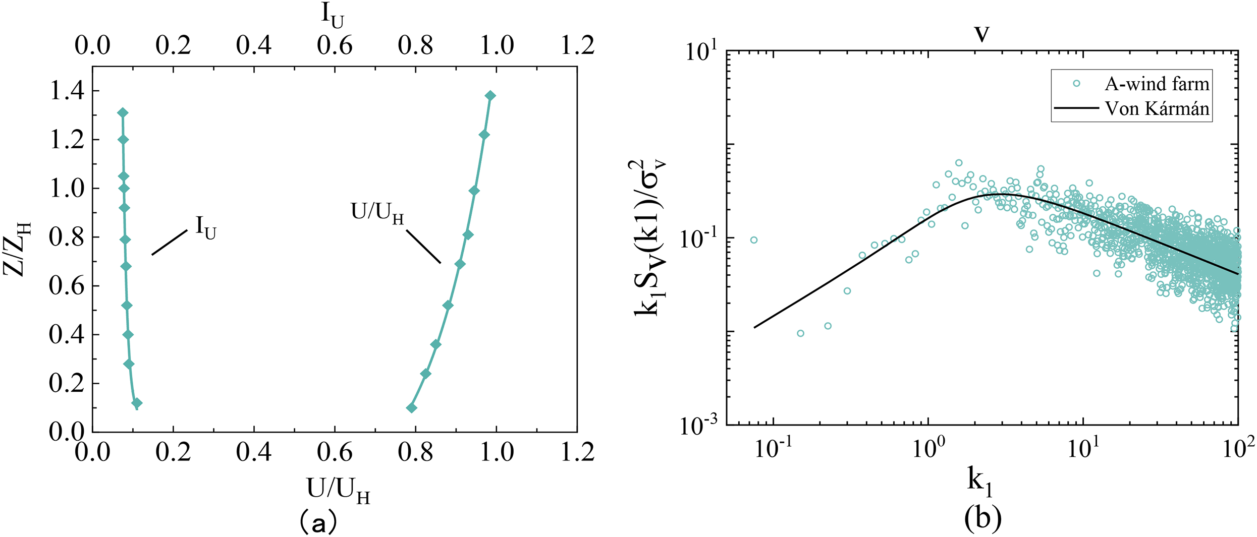
A-class atmospheric boundary layer simulated by wind tunnel tests: (a) mean velocity and intensity and (b) wind spectrum. Note: U = wind speed; Z = the height; I_U = the turbulence intensity; U_H = the model reference point wind speed; Z_H stands for the model reference point height; k1 = index of refraction.

Experiment

Model architecture

Measurements of wind pressure coefficients are frequently contaminated by environmental noise and instrumentation artifacts, introducing significant interference signals. To address this issue, the raw time-series data are initially segmented into stationary components through WT decomposition. Subsequently, a hybrid WT–CNN–LSTM–Attention predictive framework is developed, integrating CNN and RNN with attention mechanisms. Figure 6 illustrates the model's architecture, while the detailed methodological approach comprises the following key steps:

Step 1: The wind pressure coefficient measurements obtained from wind tunnel tests on the terminal building's glass curtain wall are imported as input. Preprocessing steps, including gap filling via mean interpolation, are applied to handle missing data.

Step 2: The preprocessed dataset is decomposed into multiple frequency-dependent subsets using wavelet analysis. Each subset undergoes a stationarity check. If the validation fails, decomposition parameters are iteratively refined until compliance is achieved.

Step 3: The validated wavelet components are reconstructed to isolate the low-frequency and high-frequency constituents separately.

Step 4: The hybrid CNN–LSTM–Attention architecture is utilized to separately model and predict the distinct frequency components (low-frequency and high-frequency) that were isolated during the preceding decomposition stage.

Step 5: The predictive outputs from both frequency domains are aggregated to generate the final wind pressure coefficient estimation.

Figure 6.

Model construction process of wavelet transform–convolutional neural network–long short-term memory (WT–CNN–LSTM)–attention.

Run test

Non-stationary wind pressure coefficient data often contain trend terms and fluctuation aggregation features, which need to be preprocessed to eliminate the interference of deterministic components. Firstly, a linear trend is fitted to the wind pressure coefficient series ${x_{t}}_{t = 1}^{n}$ using the least squares method:

x_{t} = α + β t + ε_{t}

(8)

where

α

and

β

are trend parameters and

ε_{t}

is the residual series. The residuals

ε_{t} = x_{t} - (\hat{α} + \hat{β} t)

are transformed into a zero-mean sequence by calculating the residuals. Subsequently, a binary sequence

{y_{t}}

is constructed based on the residual sign :

y_{t} = {\begin{matrix} 1, & if ε_{t} \geq 0 \\ 0, & if ε_{t} < 0 \end{matrix}

(9)

The non-stationary fluctuations of the wind pressure coefficients are transformed into a signed sequence, and a tour test is performed on the preprocessed binary sequence ${y_{t}}$ . The number of 1s in the sequence is set to $n_{1}$ , the number of 0s to $n_{2}$ , and the total number of tours to R. The normal approximation is used when $n_{1} \geq 10$ and $n_{1} \geq 20$ :

E (R) = \frac{2 n_{1} n_{2}}{n} + 1

(10)

Var (R) = \frac{2 n_{1} n_{2} (2 n_{1} n_{2} - n)}{n^{2} (n - 1)}

(11)

Z = \frac{R - E (R)}{\sqrt{Var (R)}}

(12)

At the significance level $α$ , if $| Z | > Z_{α / 2}$ , the null hypothesis of “sequence randomness” is rejected, indicating that the wind pressure coefficient data still exhibit non-stationary characteristics.

Wavelet transform (WT)

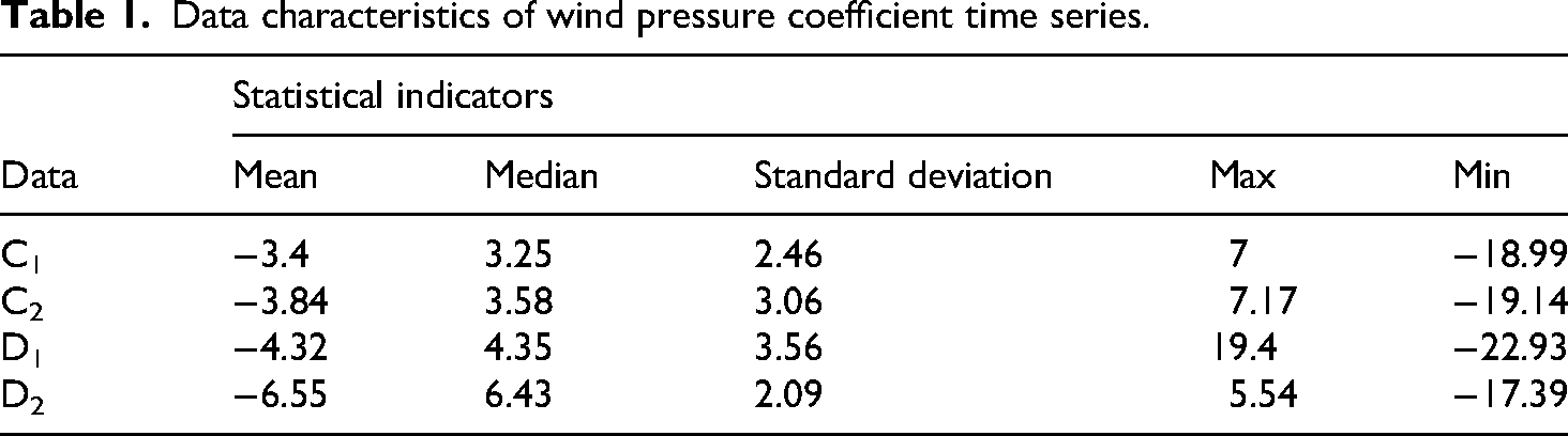
The WT is a mathematical tool for analyzing signals in the time-frequency domain, with the capability of providing both time and frequency information of signals. It is particularly well-suited for the processing of non-stationary signals, in contrast to the Fourier transform, which can only provide global frequency information. The WT is able to localize the signal through wavelet functions, which can capture the transient characteristics and detailed information of the signal on different scales. The fundamental principle of the WT hinges on the translation and scaling properties of the wavelet function, which are utilized to decompose the signal into subbands of varying frequencies through a multi-resolution decomposition of the signal. The process of wavelet decomposition typically encompasses two steps: decomposition and reconstruction. In the decomposition stage, the signal is decomposed through low-pass and high-pass filters into approximate and detail components, with the approximate component representing the low-frequency part of the signal and the detail component capturing the high-frequency part of the signal. Through the step-by-step decomposition, the signal can be decomposed into subbands at multiple scales, with each level of decomposition further refining the frequency characteristics of the signal. The reconstruction stage then follows, whereby the decomposed signal is recombined using an inverse WT, thereby recovering the original signal. The data characteristics of the raw data are displayed in Table 1.

Table 1.

Data characteristics of wind pressure coefficient time series.

	Statistical indicators
Data	Mean	Median	Standard deviation	Max	Min
C₁	−3.4	3.25	2.46	7	−18.99
C₂	−3.84	3.58	3.06	7.17	−19.14
D₁	−4.32	4.35	3.56	19.4	−22.93
D₂	−6.55	6.43	2.09	5.54	−17.39

On this basis, the probability density function (PDF) diagrams of four typical measuring points are also given, as shown in Figure 7.

Figure 7.

Probability density functions (PDFs) of fluctuating wind pressure at typical measuring points on the surface of the glass curtain wall: (a–d) point C₁, C₂, D₁, and D₂ (PDF at α = 0°).

As the wind pressure coefficient represents a discrete temporal sequence, appropriate discretization techniques are required for analysis. The proposed methodology successfully mitigates the non-stationary behavior inherent in wind pressure coefficient time series, consequently minimizing the adverse effects of data instability on prediction accuracy. This process is mainly implemented for proportional parameters and displacement parameters, with the formula referring to equation (8).

{DWT}_{f} (m, n) = α_{0}^{- m / 2} \int_{- \infty}^{+ \infty} f (t) ψ * (α_{0}^{- m} t - n τ_{0}) d t

(13)

In the formula, $α_{0}$ is the scale parameter; $τ_{0}$ is a translation parameter; m, $n$ are the scaling and translation parameters, respectively; $ψ * (x)$ is a complex conjugate function; and $f (t)$ is a time series.

The schematic diagram of the wavelet decomposition structure is shown in Figure 8. The time-frequency diagram of the wind pressure coefficient obtained by the wavelet decomposition method is shown in Figure 9.

Figure 8.

Discrete wavelet decomposition process.

Figure 9.

The time-frequency map obtained by applying the discrete wavelet transform (DWT) to the measured wind pressure coefficient sequence.

Wavelet decomposition is implemented through WT techniques, where the choice of wavelet basis functions critically influences the detection of localized signal characteristics. Standard wavelet bases such as Morlet, Daubechies, and Meyer wavelets are widely utilized in this context. Among these, the Daubechies wavelet (denoted as dbN, with N representing the wavelet order) exhibits orthogonality and demonstrates superior time-frequency localization capabilities, making it particularly suitable for noise reduction applications. In practical implementations, the dbN wavelet is typically applied using MATLAB's built-in functions. By systematically evaluating different wavelet orders through iterative refinement, the optimal db3 configuration was identified and subsequently employed to execute the decomposition procedure.

Results and discussion

In the prediction of wind pressure coefficients, the input time series of wind pressure coefficients is divided into a number of samples ${c_{t - w}, c_{t - w + 1}, \dots, c_{t}}$ , with each sample being used to predict the next wind pressure coefficient $c_{t + Δ}$ . In the actual prediction task, the window size is denoted by w and the forward step size by $Δ$ . In this study, 20% of the dataset is used for testing, and the rest of the dataset is used as part of the training set. The prediction model of wind pressure coefficient was developed by employing the back propagation technique for training, with the tests being executed on a computer with Python 3.11 framework installed. Figure 10 provides a concise overview of the primary procedure.

Figure 10.

Process of establishing wind pressure coefficient prediction models.

In this section, the focus is on four points (C₁, C₂, D₁, and D₂) located at the windward corner of the side of the glass curtain wall when the wind angle is 0°. These points are selected as the research objects. In order to highlight the advantages of the CNN–LSTM–Attention prediction model (the model structure is shown in Figure 11) proposed in this paper more effectively, the study will combine the wind pressure coefficient prediction results derived from a single CNN model and an LSTM model for comparative analysis, as shown in Figure 12.

Figure 11.

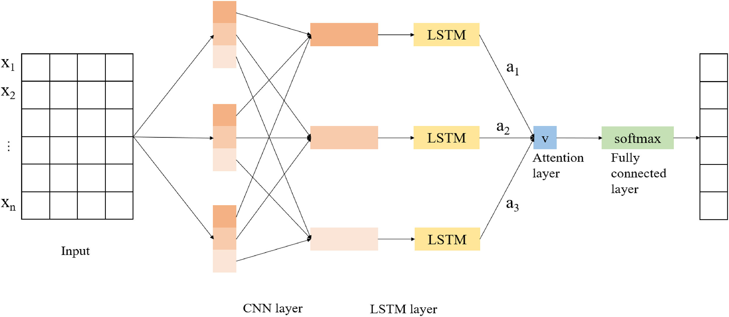
Structure of a convolutional neural network–long short-term memory (CNN–LSTM)–Attention model.

Figure 12.

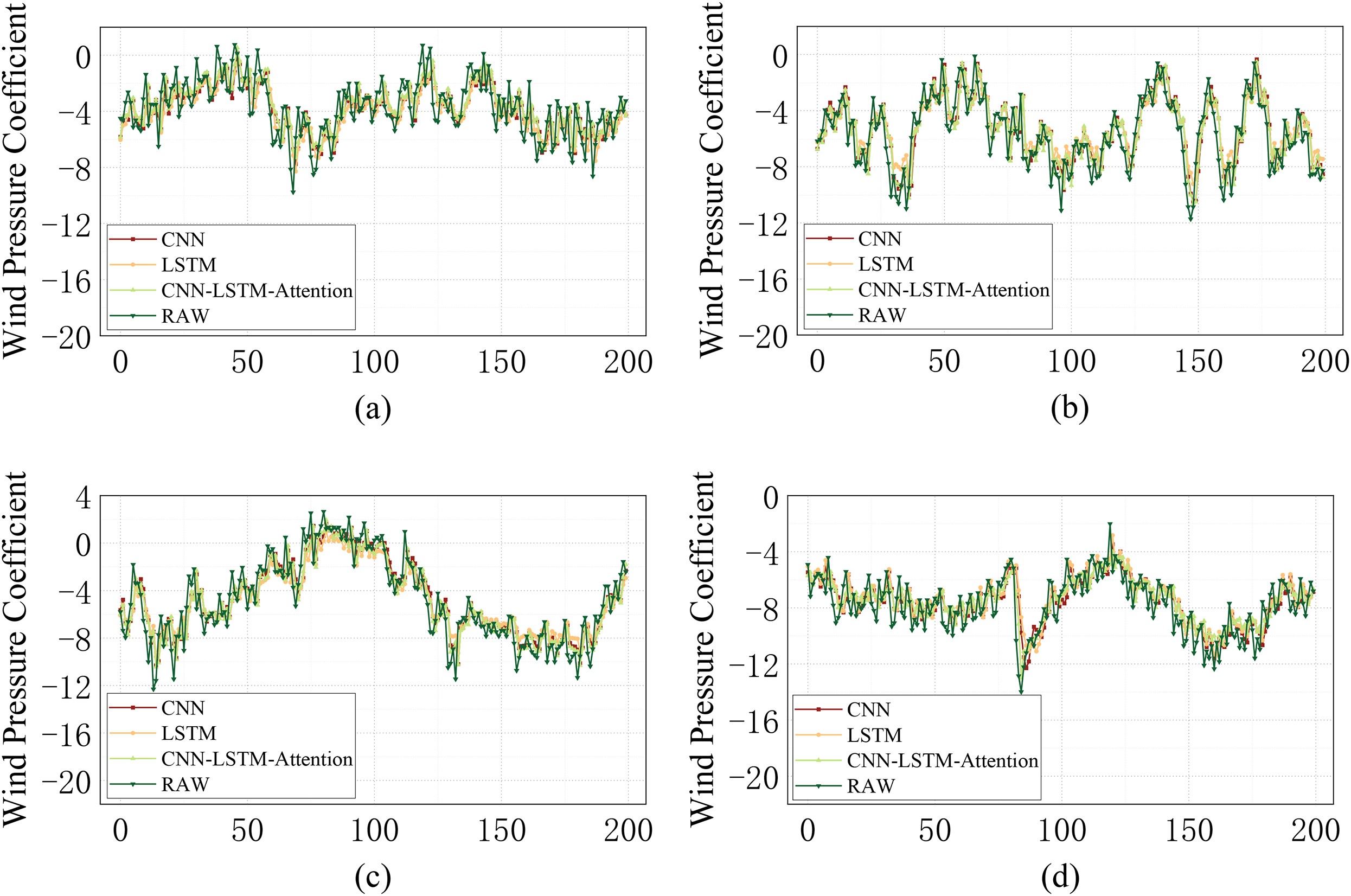
Plots of wind pressure coefficient prediction results for CNN, LSTM, and CNN–LSTM–Attention models: (a–d) correspond to the four points C₁, C₂, D₁, and D₂.

In the context of practical engineering applications, efficiency assumes paramount importance. The reduction of time loss is a key benefit of high efficiency, which is also an important factor to consider when selecting a model. As demonstrated in Figure 13, the training time of CNN, LSTM, and CNN–LSTM–Attention is shown. When there is no significant difference in the length of time, the model with higher prediction accuracy is preferred.

Figure 13.

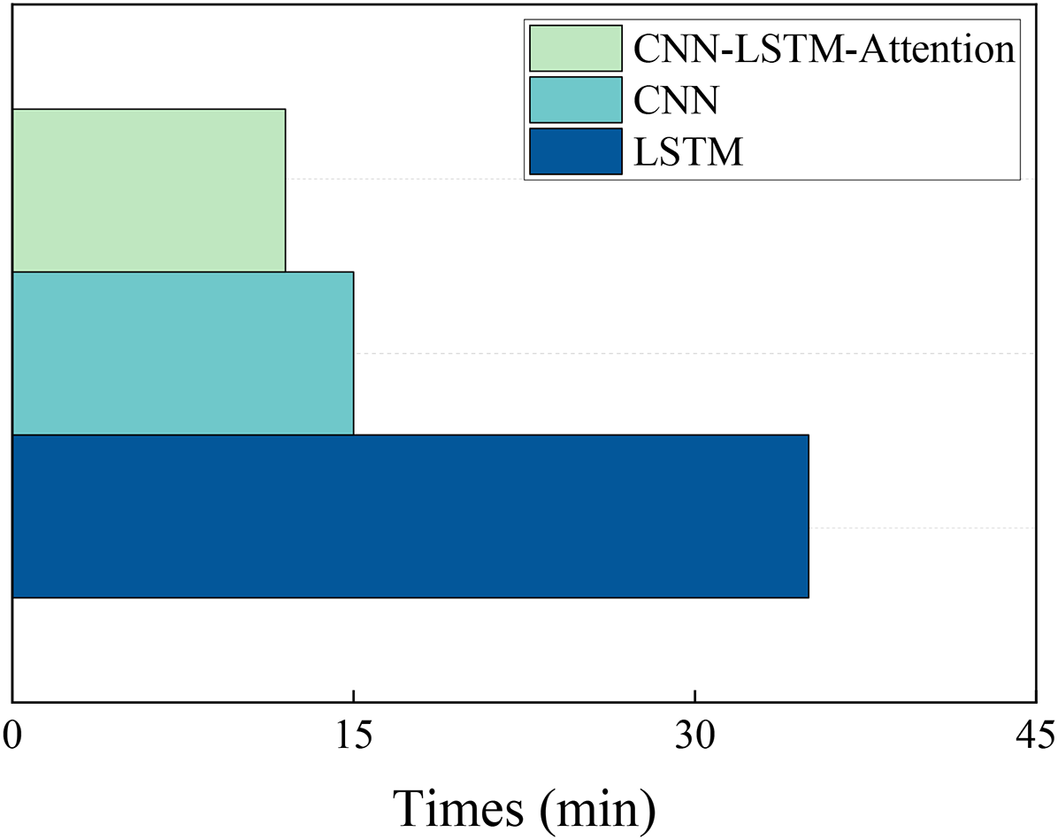
Training time diagram of different wind pressure coefficient prediction models.

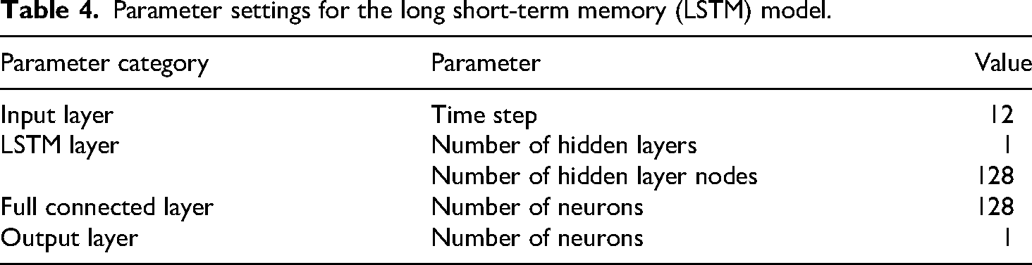
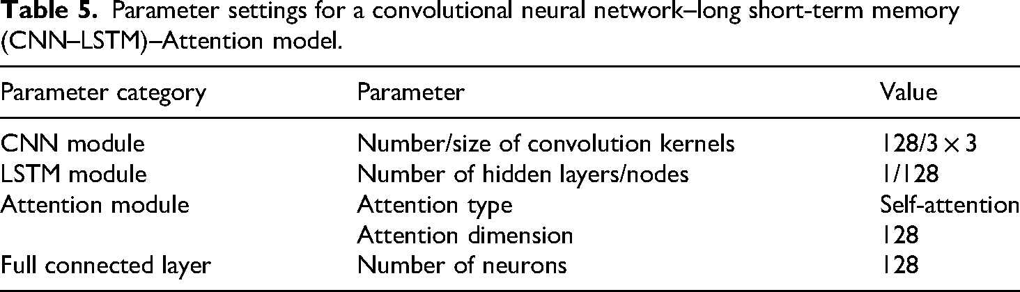
The results clearly demonstrate that each of the three models effectively captured short-term fluctuations in the wind pressure coefficient, underscoring the robust predictive performance of machine learning approaches for this application. Detailed configurations of the model parameters are provided in Tables 2 to 5.

Table 2.

Parameter settings for CNN, LSTM, and CNN–LSTM–Attention models.

Parameter	CNN	LSTM	CNN–LSTM–Attention
Input length	60	60	60
Training batch scale	32	32	32
Optimizer	Adam	Adam	Adam
Number of training iterations	30	30	30
Activation function	ReLu	ReLu	Softmax
Learning rate	1 × 10⁻⁴	1 × 10⁻⁴	1 × 10⁻⁴

CNN: convolutional neural network; LSTM: long short-term memory; ReLu: rectilinear unit.

Table 3.

Parameter settings for a convolutional neural network (CNN) model.

Parameter category	Parameter	Value
Input layer	Time step	12
Convolution layer	Number of convolution kernels	128
Convolution layer	Convolution kernel size	3 × 3
Pooling layer	Number of pooling kernels	3 × 3
Full connected layer	Number of neurons	128
Output layer	Number of neurons	1

Table 4.

Parameter settings for the long short-term memory (LSTM) model.

Parameter category	Parameter	Value
Input layer	Time step	12
LSTM layer	Number of hidden layers	1
LSTM layer	Number of hidden layer nodes	128
Full connected layer	Number of neurons	128
Output layer	Number of neurons	1

Table 5.

Parameter settings for a convolutional neural network–long short-term memory (CNN–LSTM)–Attention model.

Parameter category	Parameter	Value
CNN module	Number/size of convolution kernels	128/3 × 3
LSTM module	Number of hidden layers/nodes	1/128
Attention module	Attention type	Self-attention
Attention module	Attention dimension	128
Full connected layer	Number of neurons	128

A random sampling and visualization of the loss functions of the different predictive models used during the training process at the four measurement points was carried out through several experiments, as shown in Figure 14. The findings demonstrate that the choice of learning rate has a significant impact on model convergence during the training process of neural network models. Specifically, an elevated learning rate has been shown to expedite the initial convergence of the model, although it has also been observed to induce oscillations during the training process and potentially impact the convergence of the model to the global optimal solution. Conversely, a reduced learning rate has been demonstrated to ensure the stability of the training process, albeit with a substantial reduction in convergence speed of the model. In light of these findings, this study sets the learning rate to 1 × 10⁻⁴ as the convergence condition for model training through systematic parameter adjustment. The results demonstrate that this learning rate setting can effectively balance the training speed and stability, with the model reaching a stable state after approximately 30 rounds of iterations. It is evident that the CNN–LSTM–Attention model exhibits the fastest convergence speed, the CNN model exhibits the second fastest convergence speed, and the LSTM model exhibits the slowest convergence speed.

Figure 14.

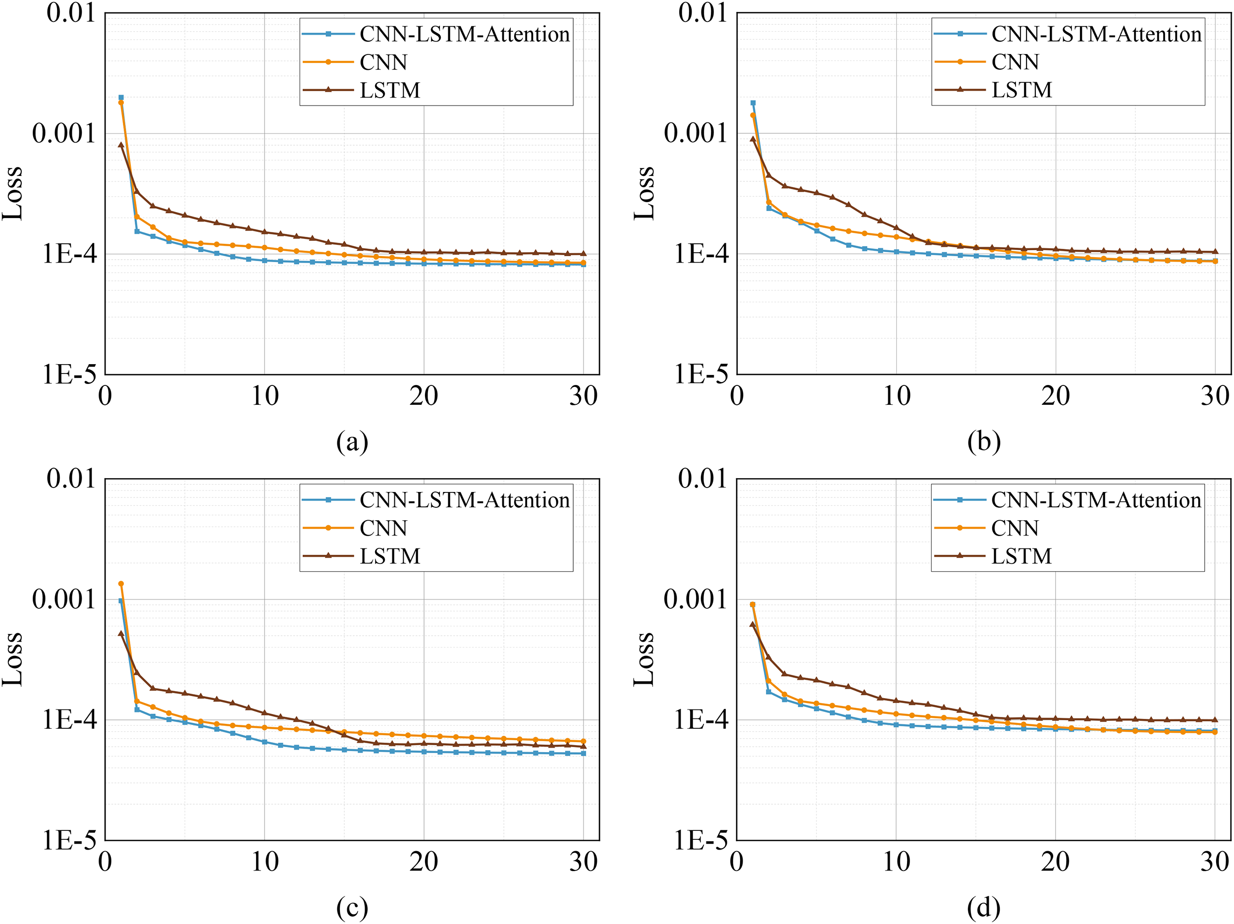
The loss function diagrams of CNN, LSTM, and CNN–LSTM–Attention models: (a–d) correspond to the four points C₁, C₂, D₁, and D₂.

Whilst all three types of models demonstrate effective prediction capabilities for wind pressure coefficients, it is evident from the prediction plots that the CNN–LSTM wind pressure coefficient prediction model, incorporating the attention mechanism proposed in this study, exhibits superior numerical convergence with the original wind pressure coefficient sequences when compared with the single prediction model. It is noteworthy that all evaluations are objective and substantiated by empirical evidence. The CNN–LSTM–Attention model demonstrates superior performance in the prediction of extreme points, exhibiting a more pronounced agreement with the original data curves. This suggests that the model exhibits excellent prediction capabilities. Following a series of training and testing comparisons, it can be concluded that the CNN–LSTM–Attention model maintains a consistent and reliable prediction accuracy, devoid of any significant fluctuations. Consequently, this paper asserts that the CNN–LSTM–Attention model exhibits superior prediction accuracy.

To further explore the impact of the wavelet decomposition technique in the prediction of non-stationary wind pressure coefficient sequences, the four points C₁, C₂, D₁, and D₂ mentioned above will be used as an example. The WT is applied to the original wind pressure coefficient sequence to ensure that the decomposed components can pass the traveling test. The high-frequency components are then reconstructed as U, and the low-frequency components are reconstructed as L, which are inputted into the CNN–LSTM–Attention model, respectively. The results are then summed up and compared with the results obtained when the original wind pressure coefficient sequence, which has not been decomposed by the wavelet decomposition, is imported into the CNN–LSTM–Attention model. The results are observed in comparison with the results obtained in the model, and the results are shown in Figure 15.

Figure 15.

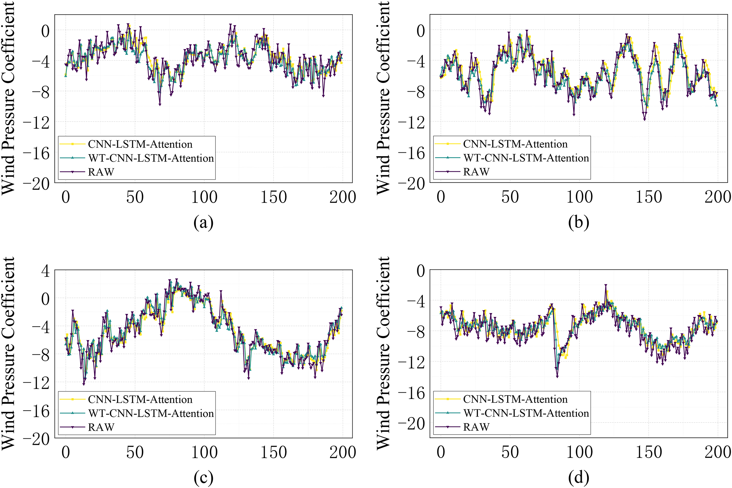
Plot of wind pressure coefficient prediction results for CNN–LSTM–Attention and WT–CNN–LSTM–Attention models: (a–d) corresponds to four points C₁, C₂, D₁, and D₂.

As demonstrated in the figure, the CNN–LSTM–Attention model has been shown to be superior to the single prediction model in terms of prediction accuracy. However, the WT–CNN–LSTM–Attention model has been observed to demonstrate a higher degree of convergence in the prediction of specific peaks and valleys. Through repeated iterations of the test, the WT–CNN–LSTM–Attention model has repeatedly demonstrated a higher degree of curve fit to the original wind pressure coefficient series. In light of the preceding discourse on the utilization of diverse models for wind speed prediction, the wavelet-based CNN–LSTM–Attention model proposed in this study is deemed to be the most efficacious.

Assessment of methods for predicting wind pressure coefficient

For a comprehensive evaluation of the proposed model's predictive performance, three quantitative metrics are employed: mean absolute error (MAE), RMS error (RMSE), and mean absolute percentage error (MAPE). These evaluation criteria are mathematically expressed as:

MAE = \frac{1}{T} \sum_{t = 1}^{T} | N_{t} - {\hat{N}}_{t} |

(14)

RMSE = \sqrt{\frac{1}{T} \sum_{t = 1}^{T} {(N_{t} - {\hat{N}}_{t})}^{2}}

(15)

MAPE = \frac{1}{T} \sum_{t = 1}^{T} | \frac{N_{t} - {\hat{N}}_{t}}{N_{t}} |

(16)

In the formula, $N_{t}$ corresponds to the measured value at temporal instance t, ${\hat{N}}_{t}$ indicates the model's predicted output for the same time step t, ${\bar{N}}_{t}$ represents the arithmetic mean of all observed measurements, and T specifies the total number of prediction points in the testing dataset.

In this section, the MAE, RMSE, and MAPE error indices of the four points C₁, C₂, D₁, and D₂ are calculated using different prediction models. The prediction performance of each model is then compared quantitatively, and the error results of multiple trials are plotted as a graph.

As illustrated in Table 6 and Figure 16, among the three types of models without wavelet decomposition, the CNN–LSTM–Attention model demonstrates the optimal performance in the three error metrics of MAE, RMSE, and MAPE. The CNN model exhibits the second-best performance, while the LSTM model shows the least optimal performance. For C1, the lowest MAE of the CNN–LSTM–Attention model is 1.15, which is optimized by 0.03 to 0.10 compared to CNN and LSTM; the lowest RMSE is 1.41, which is optimized by 0.02 to 0.09 compared to CNN and LSTM; the lowest MAPE is 0.69, which is optimized by 0.07 to 0.11 compared to CNN and LSTM. For the remaining three points, C2, D1, and D2, the CNN–LSTM–Attention model is also optimized to different degrees compared with CNN and LSTM in the three error metrics. This shows that the CNN–LSTM hybrid model with the introduction of the attention mechanism has a better overall performance in predicting the wind pressure coefficient sequence.

Figure 16.

Error diagram of wind pressure coefficient prediction results for CNN, LSTM, and CNN–LSTM–Attention models: (a–d) corresponding to four points C₁, C₂, D₁, and D₂.

Table 6.

Summary of error in wind pressure coefficient prediction using CNN, LSTM, and CNN–LSTM–Attention models at different points.

Point	Index	Model
C₁	MAE	CNN	1.18
		LSTM	1.25
		CNN–LSTM–Attention	1.15
	RMSE	CNN	1.43
		LSTM	1.50
		CNN–LSTM–Attention	1.41
	MAPE	CNN	0.76
		LSTM	0.80
		CNN–LSTM–Attention	0.69
C₂	MAE	CNN	1.15
		LSTM	1.17
		CNN–LSTM–Attention	1.12
	RMSE	CNN	1.46
		LSTM	1.48
		CNN–LSTM–Attention	1.42
	MAPE	CNN	0.41
		LSTM	0.42
		CNN–LSTM–Attention	0.38
D₁	MAE	CNN	1.25
		LSTM	1.31
		CNN–LSTM–Attention	1.20
	RMSE	CNN	1.58
		LSTM	1.65
		CNN–LSTM–Attention	1.54
	MAPE	CNN	0.59
		LSTM	0.67
		CNN–LSTM–Attention	0.56
D₂	MAE	CNN	1.01
		LSTM	1.03
		CNN–LSTM–Attention	0.99
	RMSE	CNN	1.26
		LSTM	1.32
		CNN–LSTM–Attention	1.23
	MAPE	CNN	0.14
		LSTM	0.15
		CNN–LSTM–Attention	0.11

CNN: convolutional neural network; LSTM: long short-term memory; MAE: mean absolute error; RMSE: root mean square error; MAPE: mean absolute percentage error.

Next, for the non-stationarity of the wind pressure coefficient sequence, the CNN–LSTM–Attention model with and without passing wavelet decomposition as the control group is set up, and quantitative analysis is performed to analyze the prediction results of the two. As can be seen in Figure 17, the WT–CNN–LSTM–attention prediction model also performs well in the three error metrics, MAE, RMSE, and MAPE, with MAE of 1.00 to 1.12, RMSE of 1.19 to 1.38, and MAPE of 0.13 to 0.60. Compared with the CNN–LSTM–Attention model, the MAE was optimized by 0.20 to 0.22, RMSE by 0.19 to 0.23, and MAPE by 0.11 to 0.21. It can be seen that the original non-stationary wind pressure coefficient sequences are reconstructed into high-frequency and low-frequency sequences by wavelet decomposition, and then imported into the CNN–LSTM–Attention model, respectively, and the summed results are significantly better than those of the scheme that is directly predicted without wavelet decomposition.

Figure 17.

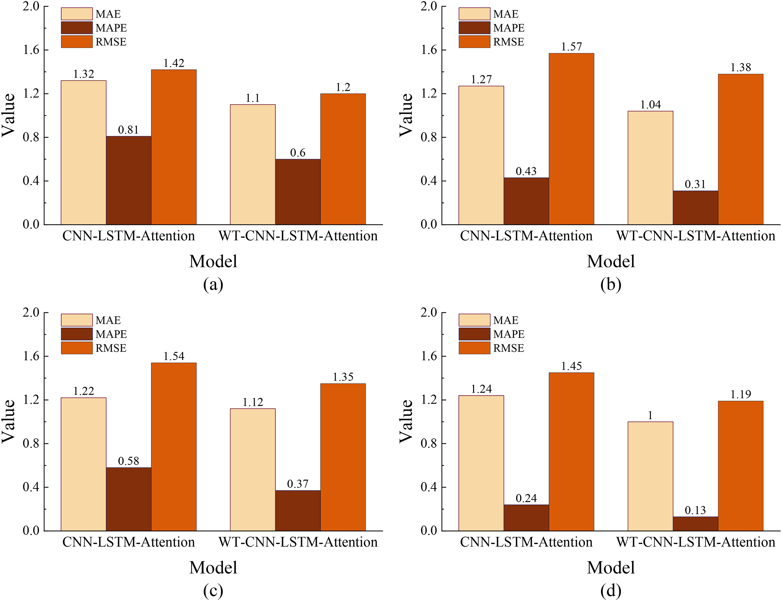
Error diagram of wind pressure coefficient prediction results for CNN–LSTM–Attention and WT–CNN–LSTM–Attention models: (a–d) corresponding to four points C₁, C₂, D₁, and D₂.

In order to further verify the robustness of the prediction ability of the WT–CNN–LSTM–Attention model, the typical measurement points C₁, C₂, D₁, and D₂ at 45° and 90° wind angles will continue to be tested. The results are displayed in the accompanying figure. As illustrated in Figure 18, the WT–CNN–LSTM–Attention model consistently demonstrates optimal prediction accuracy when employed to predict four measuring points at three distinct wind directions. In comparison with the model that does not involve wavelet decomposition, the WT–CNN–LSTM–Attention model has been shown to possess a number of significant advantages. It can thus be concluded that the WT–CNN–LSTM–Attention model is a more stable model when employed for the purpose of predicting wind pressure coefficient, and that it is suitable for prediction scenarios involving different wind directions.

Figure 18.

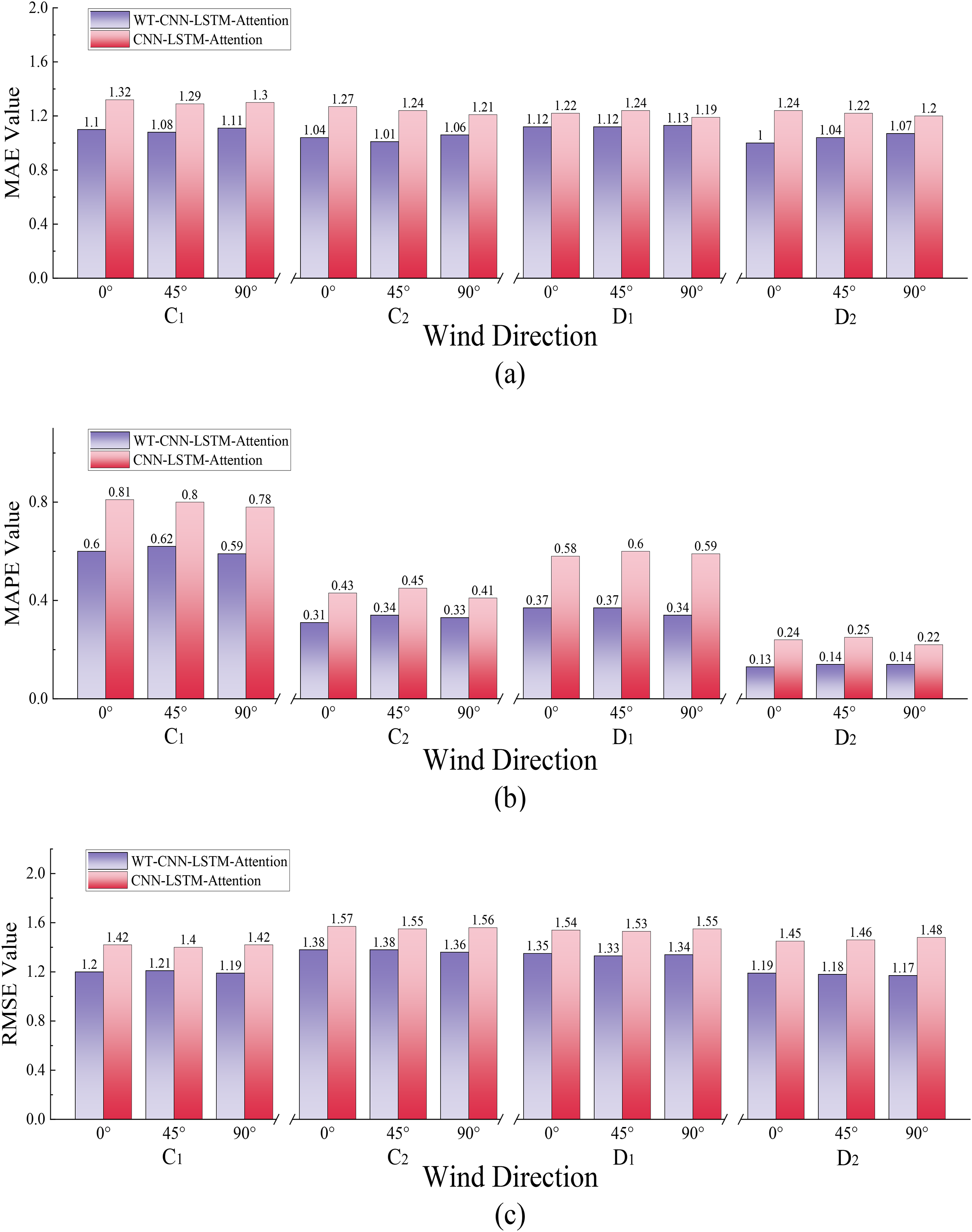
Error diagram of typical measuring points C₁, C₂, D₁, and D₂ at 0°, 45°, and 90° wind directions: (a–c) corresponds to MAE, MAPE, and RMSE.

Error analysis based on reality

The glass curtain wall structure is distinguished by its lightweight nature and permeability. The panel and support structure are interconnected, and the structure is vulnerable to wind pressure. The distribution of wind pressure is heterogeneous and pulsating, both spatially and temporally, due to the interference effect of building shape, height, and the surrounding environment. In this context, in addition to the individual differences of different neural network prediction models, the causes of errors may come from:

The structural parameters of glass curtain walls are intricate, with considerations including panel dimensions, keel stiffness, and connection method. In the event that the training data do not fully cover the actual parameter combination of the project, the model's generalization ability is limited.

It is important to note that the distribution of wind pressure is affected by nonlinear factors, including turbulence and interference effects. Should the model fail to accurately capture the complex mapping relationship between wind pressure and structural response (e.g. by ignoring local wind pressure mutations caused by interference), this can lead to prediction deviation.

The limitations of data acquisition must be considered. Such limitations may include insufficient on-site monitoring samples, differences between wind tunnel test conditions and actual environmental conditions, or the simplification of the computational fluid dynamics (CFD) simulated turbulence model. These factors may result in a disconnection between the training data and real working conditions.

The aforementioned error sources have been demonstrated to exert a substantial influence on the evaluation of project safety. It is imperative to accurately gauge wind pressure in structural design, as overestimation can lead to redundancy and escalate construction costs. Conversely, underestimation can compromise the structural integrity of glass curtain walls, potentially resulting in safety hazards such as panel rupture and connector failure, particularly in extreme conditions such as typhoons and strong winds. Furthermore, an inaccurate prediction of the abnormal wind pressure caused by the interference effect may result in the failure to inspect local weak areas, thereby compromising the safety of the building. It is imperative that future research endeavors are initiated from a multitude of perspectives to ensure the safety of the project. This involves the integration of field measurement and CFD simulation to generate multi-source data, the refinement of structural characteristic parameters of the glass curtain wall, the optimization of neural network model structure, and the enhancement of prediction accuracy. These measures are essential to establish a reliable foundation for the wind-resistant design and safety assessment of the terminal glass curtain wall.

Conclusions

This paper proposes a CNN–LSTM combinatorial model with wavelet decomposition and an attention mechanism for short-term wind pressure coefficient prediction. Developed using wind tunnel test data from an airport terminal's glass curtain wall, the model undergoes iterative training and comprehensive error analysis to assess its predictive capability. Comparative evaluations with standalone CNN, LSTM, and a wavelet-free integrated model show:

The study addresses the lack of research on wind pressure coefficients for terminal building glass curtain walls, providing references for safety assessments.

Treating wind pressure coefficient sequences as non-stationary signals achieves satisfactory prediction results, with the wavelet-decomposed CNN–LSTM–Attention model demonstrating stronger performance and generalization ability.

Error metrics across the curtain wall surface confirm that the attention-integrated CNN–LSTM model outperforms single prediction models in wind pressure coefficient prediction.

Supplemental Material

sj-docx-1-sci-10.1177_00368504251366365 - Supplemental material for A convolutional neural network–long short-term memory (CNN–LSTM)–Attention model based on wavelet transform for predicting non-stationary wind pressure coefficients on the surface of terminal glass curtain wall

Supplemental material, sj-docx-1-sci-10.1177_00368504251366365 for A convolutional neural network–long short-term memory (CNN–LSTM)–Attention model based on wavelet transform for predicting non-stationary wind pressure coefficients on the surface of terminal glass curtain wall by Yuxuan Bao, Cheng Pei, Yuhao Mou, Mingjie Li and Xiaokang Cheng in Science Progress

Footnotes

ORCID iD

Yuxuan Bao

Author contributions

Yuxuan Bao: Writing—original draft. Cheng Pei: Writing—review and editing. Yuhao Mou: Software. Mingjie Li: Methodology. Xiaokang Cheng: Supervision.

Funding

The authors disclosed receipt of the following financial support for the research, authorship, and/or publication of this article: This work was supported by the Fundamental Research Funds for the Central Universities (24CAFUC05004); the Fundamental Research Funds for the Central Universities (25CAFUC10023); the Fundamental Research Funds for the Central Universities (24CAFUC03037); Sichuan Provincial Engineering Research Center of Smart Operation and Maintenance of Civil Aviation Airports (JCZX2023ZZ03); National Key Research and Development Program of China (2022YFC3005301).

Declaration of conflicting interests

The authors declared no potential conflicts of interest with respect to the research, authorship, and/or publication of this article.

Data availability

The data that support the findings of this study are available on request from the corresponding author. The data are not publicly available due to privacy.

Supplemental material

Supplemental material for this article is available online.

References

Uematsu

Tsuruishi

. Wind load evaluation system for the design of roof cladding of spherical domes. J Wind Eng Ind Aerodyn 2008; 96: 2054–2066.

Dongmei

Shiqing

Xuhui

, et al. Prediction of wind loads on high-rise building using a BP neural network combined with POD. J Wind Eng Ind Aerodyn 2017; 170: 1–17.

Bre

Gimenez

Fachinotti

. Prediction of wind pressure coefficients on building surfaces using artificial neural networks. Energy Build 2018; 158: 1429–1441.

Liu

Tao

, et al. Deep learning-based investigation of wind pressures on tall building under interference effects. J Wind Eng Ind Aerodyn 2020; 201: 104138.

Liu

Wang

, et al. Wind speed point prediction and interval prediction method based on linear prediction model, neural network, and deep learning. J Ambient Intell Humaniz Comput 2022; 14: 9207–9216.

. Short-term wind speed forecasting based on two-stage preprocessing method, sparrow search algorithm and long short-term memory neural network. Energy Rep 2022; 8: 14997–15010.

Wang

. A hybrid neural network model for short-term wind speed forecasting. Energies 2023; 16: 1841–1841.

Wang

. Wind speed interval prediction based on multidimensional time series of convolutional neural networks. Eng Appl Artif Intell 2023; 121: 105987.

Nascimento

EGS

de Melo

TAC

Moreira

. A transformer-based deep neural network with wavelet transform for forecasting wind speed and wind energy. Energy 2023; 278: 127678.

10.

Barjasteh

Hamid Ghafouri

Hashemi

. A hybrid model based on discrete wavelet transform (DWT) and bidirectional recurrent neural networks for wind speed prediction. Eng Appl Artif Intell 2024; 127: 107340.

11.

Joseph

Deo

Pérez

, et al. Short-term wind speed forecasting using an optimized three-phase convolutional neural network fused with bidirectional long short-term memory network model. Appl Energy 2024; 359: 122624.

12.

Ali

Aly

. Short term wind speed forecasting using artificial and wavelet neural networks with and without wavelet filtered data based on feature selections technique. Eng Appl Artif Intell 2024; 133: 108201.

13.

Huang

, et al. Convolutional neural network-based wind pressure prediction on low-rise buildings. Eng Struct 2024; 309: 118078.

14.

Jung

. Data-driven prediction of wind pressure on low-rise buildings in complex heterogeneous terrains. Build Environ 2024; 265: 112022.

15.

Cao

Wang

, et al. Scientific preparation for JRT: wind pressure prediction model for large radio telescope based on real data from multi-sensors. Heliyon 2024; 10: e37892.

16.

Wang

Shen

Wei

, et al. An intelligent framework for deriving formulas of aerodynamic forces between high-rise buildings under interference effects using symbolic regression algorithms. Build Eng 2025; 99: 111614.

17.

Wei

Shen

Wang

, et al. Transfer learning framework for the wind pressure prediction of high-rise building surfaces using wind tunnel experiments and machine learning. Build Environ 2025; 271: 112620.

18.

Zhao

Xie

Chen

. A novel nested BO–LM–BPNN method for wind pressure field prediction of non-isolated low-rise buildings. Wind Eng Ind Aerodyn 2025; 259: 106047.

19.

Ren

Liu

Wang

, et al. Spatiotemporal wind pressure field prediction for long-span flexible photovoltaic structures using deep learning and sparse wind tunnel data. Sol Energy 2025; 286: 113192.

20.

Zheng

Tang

Chen

. Research on wind pressure time history prediction of high-rise buildings based on SSA-LSTM. Chongqing Architecture 2025; 24: 64–68.

Supplementary Material

Please find the following supplemental material available below.

For Open Access articles published under a Creative Commons License, all supplemental material carries the same license as the article it is associated with.

For non-Open Access articles published, all supplemental material carries a non-exclusive license, and permission requests for re-use of supplemental material or any part of supplemental material shall be sent directly to the copyright owner as specified in the copyright notice associated with the article.

0.00 MB

0.02 MB