Sage Journals: Discover world-class research

Abstract

High-formwork support systems (HFSSs) play a crucial role in constructing complex projects. However, insufficient monitoring techniques can sometimes lead to catastrophic failures of these structures. This study presents an integrated framework for monitoring HFSS that combines numerical simulation, deep learning, and a Retrieval-Augmented Generation (RAG) system. A finite element model of HFSS was first developed and optimized using a Genetic Algorithm-Particle Swarm Optimization hybrid algorithm, generating structural response data for three critical conditions: Normal operation, local instability, and global instability. These datasets were then used to train a Recurrent Neural Network Long Short-Term Memory (RNN-LSTM) network, which can correctly predict the working states of the structure. Moreover, the effectiveness of RNN-LSTM and convolutional neural network (CNN) was compared. The results demonstrated that RNN-LSTM has superior performance over CNN in predicting the working status of HFSS. Furthermore, the study developed an RAG system incorporating GPT technology and a domain-specific knowledge graph to automate structural health monitoring (SHM) report generation. Several assessment metrics were involved to evaluate the RAG model's performance. The findings indicate that the RAG model could generate accurate and reasonable SHM reports for HFSS.

Keywords

Finite element model updating recurrent neural network long short-term memory high-formwork support system condition monitoring retrieval-augmented generation knowledge graph

Introduction

High-formwork support systems (HFSSs) are very important in construction, especially in complex structures. However, in spite of their importance, these systems may be underestimated and result in disastrous failures in certain cases. This may lead to severe economic losses and casualties.^1–3 It is paramount that the HFSS have assurance of safety management. Specifically, a timely monitoring strategy should be adopted upon operation, to determine the structural performance. In response to these needs, this study offers a new monitoring method for HFSS, based on structural response information, for example pole displacements as well as vibration signals. Such measurements hold critical information about the operational condition, through which possible risks could be identified in a timely manner.

Based on the previous study results, the effectiveness of deep learning (DL) in evaluating structural conditions has been proven.⁴ However, a major challenge in training DL techniques is the acquisition of adequate training data, especially when an application deals with a large or complicated structure, where experimental testing is not feasible due to safety considerations or high cost. Training data can be attained from numerical simulations. However, discrepancies typically exist between finite element model (FEM) results and results obtained from an experiment. The established FEM is usually required to be optimized. One of the most essential steps during the optimization process is to set appropriate values for the model updating parameters. Initial uncertainty in parameter values necessitates iterative optimization approaches to identify optimal values that minimize discrepancies between model predictions and experimental measurements.^5,6 The optimized FEM could generate datasets of both normal and abnormal stages of the operation of the structures. This process significantly reduces experimental costs and resource requirements.

This paper proposes a new FEM-informed recurrent neural network long short-term memory (RNN-LSTM) model to predict the working status of the HFSSs. The approach comprises four key phases: First, a parameterized FEM of the HFSS was created and verified. This optimized FEM model was subsequently used to generate comprehensive simulation datasets representing different working conditions of the HFSS.

These simulated datasets were then used to train the RNN-LSTM network. Then the proposed RNN-LSTM model was rigorously validated through the test measurement based on a real 8-meter-high HFSS structure. The main stages of the framework are listed below. The entire sequence is described in Figure 1.

FEM development and optimization: An FEM of the HFSS with high-fidelity was developed and then optimizsed using genetic algorithm-particle swarm optimization (GA-PSO) algorithm.

Numerical dataset generation: The parameters of the calibrated FEM were used to generate simulation data, which included a set of diverse structural response scenarios.

Implementation of DL: An appropriate RNN-LSTM architecture was selected and trained based on the comprehensive FEM-generated data set.

Experimental validation: RNN-LSTM classifier was validated against test measurements to ensure the model could provide the correct classification.

Figure 1.

The framework of the suggested approach.

The site management practitioners use primarily personal observations, experience and group knowledge to prepare the structural health monitoring (SHM) reports of the HFSS irrespective of the guidelines, standards, and regulations. It is hard to present such text information and process it in a digital format, missing the required information. These limitations underscore the critical need for standardized SHM reports containing essential, actionable data. To comprehensively assess HFSS operational conditions, this study proposed a method to automatically generate SHM report for the HFSS.

The use of large language models (LLMs) offers significant potential to streamline the documentation generation processes as they can classify documents, interpret textual content, generate reports, and extract key insights.⁷ This study aims to develop a Retrieval-Augmented Generation (RAG) framework combining LLM and SHM-specific knowledge graph (KG) to automatically generate an SHM report for HFSS. A benchmark comparison of the proposed model and GPT-4 is performed.

The “Literature review” section provides a concise review of related literature. The details of the FEM updating (FEMU) are given in the “FEM calibration” section. The study describes the training scheme of the RNN-LSTM on the simulated datasets, and experimentally validating the RNN-LSTM is provided in the “RNN-LSTM model training and experimental validation” section. This section also compares the performance of the RNN-LSTM and convolutional neural network (CNN) with regard to the measurements in the experiments. The “Development process of the RAG model” section describes the RAG model development process in generating the SHM report together with the HFSS. The “Verification of the developed RAG model” section shows the validation of the developed RAG model. The “Conclusion” section presents the conclusion.

Literature review

Finite element model updating

Although FEM serves as a powerful computational tool for structural monitoring, remaining service life prediction, damage identification, and maintenance strategy optimization, it has inherent errors and uncertainties. These uncertainties typically originate from three primary sources: Parameter variability, structural idealization discrepancies, and numerical implementation limitations.⁸

FEMU is fundamentally an optimization process aimed at reducing discrepancies between numerical simulations and actual structural behavior. Conventional FEMU methodologies typically incorporate experimental data obtained through static and/or dynamic testing of the physical structure. The approach involves constructing an objective function that quantifies various forms of discrepancies between computational results and experimental measurements. The employed datasets may consist of static response measurements,^9–12 dynamic characteristics,^13–20 or hybrid combinations of both data types.^21–25

Iterative FEM updating algorithms are based on the adoption of changes in structural parameters and optimization methods to generate realistic and reasonable results.²⁶ These algorithms are usually based on dealing with an optimization problem for which optimization methods are employed to explore the global optimum. Genetic algorithm (GA) and particle swarm optimization (PSO) algorithms are most commonly used, but there are several algorithms also available in FEMU, including gray wolf,²⁷ harmony search,²⁸ gravitational search,²⁹ colliding bodies,³⁰ and simulated annealing.³¹

In this study, the FEMU process can be divided into the selection of updating model parameters, the setup of the tests on real structure and the availability of experimental measurements, the formulation of the objective function, and the selection of optimization approach. Commercially available software packages were adopted to create and optimize the model. Moreover, a full-scale HFSS was built to provide experimental measurements that are essential during the finite element (FE) updating process. A comparative analysis was conducted among multiple optimization algorithms, including GA-PSO, GA, gradient-based optimization (GBO), and gray wolf optimizer (GWO), to identify the most effective approach.

Hybrid DL methods

DL methods are good at exploring the relationships in complex, high-dimensional data, which makes them able to be employed in many fields, including fault detection, forecasting and prediction, health monitoring, and image processing.³² In addition, it was demonstrated that they can be successfully used in SHM and damage detection.^33–36

Recently, hybrid DL approaches have attracted considerable interest within the construction industry.³⁷ Li et al.³⁸ proposed a hybrid DL algorithm (CNN-BiLSTM-Adaboost) to predict HFSS displacement and load. The model achieved an R² score of over 98%, surpassing both standalone DL methods: CNN (93%) and BiLSTM (91%). Rathod et al.³⁹ also used a hybrid method to assess the damage severity of the structure by using FEM simulated data. FEM was adopted to provide training data for the hybrid DL algorithm in terms of various cases of damage involved in structures. Based on the study results, the proposed method could successfully explore the complex relationships between inputs and outputs. Madhusudhanan et al.⁴⁰ developed a hybrid DL method to evaluate structural strength conditions. When tested on a structural database, the proposed approach achieved high performance. The results highlight the importance of a hybrid DL method in accurately predicting building strength. Similarly, Fuentes et al.⁴¹ introduced a novel hybrid DL network (CNN-LSTM) to predict damage zone area in a seismic event. HybridNet demonstrated improved accuracy compared with single DL methods.

Based on previous studies, hybrid DL methods—which leverage the complementary strengths of different DL architectures—can enhance both the accuracy and robustness of predictions. Therefore, this study employs a hybrid DL approach to predict the working status of the HFSS. Although hybrid DL methods show great potential, their performance is highly dependent on the completeness and accuracy of the dataset. Thus, this study used an optimized FE Method (FEM) to generate high-quality data for model training.

LLMs and RAG

Through training on massive corpora, LLMs acquire advanced abilities in text categorization,^42,43 summarization, and generation.⁴⁴ However, GPT variants display limited domain-specific understanding despite their general linguistic competence, along with concerning hallucination tendencies. Study⁴⁵ demonstrates the potential of generative artificial intelligence (AI) (ChatGPT) to assist in FE-based structural analysis and design, while highlighting critical challenges in ensuring the reliability of AI-generated solutions for safety-sensitive engineering applications. Notably, Prieto et al.⁴⁶ used GPT in schedule planning for construction projects. Uddin et al.⁴⁷ applied GPT in construction safety training. They both identified that conventional LLMs frequently generate erroneous or hallucinated outputs due to insufficient domain-specific training data.

While LLMs often demonstrate limitations in factual knowledge retention, KGs provide explicitly structured representations of factual relationships. This complementary relationship enables synergistic integration, where KGs’ structured contextual framework enhances LLMs’ semantic understanding and response accuracy.

The RAG framework significantly improves LLMs’ information retrieval and precise knowledge application capabilities. This innovative architecture addresses LLMs’ limitations in domain-specific knowledge manipulation by dynamically accessing external knowledge sources, largely improving the relevance, accuracy, efficiency, and depth of its responses. Afzal et al.⁴⁸ and Siriwardhana et al.⁴⁹ addressed RAG as allowing retrieval of information from an external database, and easing hallucination problems in construction education. Taiwo et al.⁵⁰ developed a RAG model using contract documents, which improves the abilities of GPT-4 in the field of construction contracts. Contract documents were processed into a structured database and into embedding vectors. The developed RAG model used semantic similarity in the database to produce relevant responses. The results proved higher quality compared to the standalone GPT-4 model, and the developed RAG model alleviated the hallucination issues.

While numerous LLMs exist, their application to SHM remains limited by critical challenges such as hallucination tendencies, domain-specific knowledge gaps, data constraints, and interoperability issues. This research bridges existing gaps by developing a RAG model tailored for SHM of high-formwork systems. The model leverages a domain-specific knowledge base integrated with SHM-focused KGs to enhance retrieval accuracy. Designed to generate contextually relevant and technically precise outputs for SHM applications, the proposed framework is rigorously evaluated using quantitative performance metrics.

FEM calibration

This section presents the theoretical framework for calibrating FEMs of HFSSs, accounting for semi-rigid joints and initial defects. Experimental data from a full-scale high-formwork system were utilized to validate and refine the numerical model. The calibration process, illustrated in Figure 2, involves the following key steps:

Figure 2.

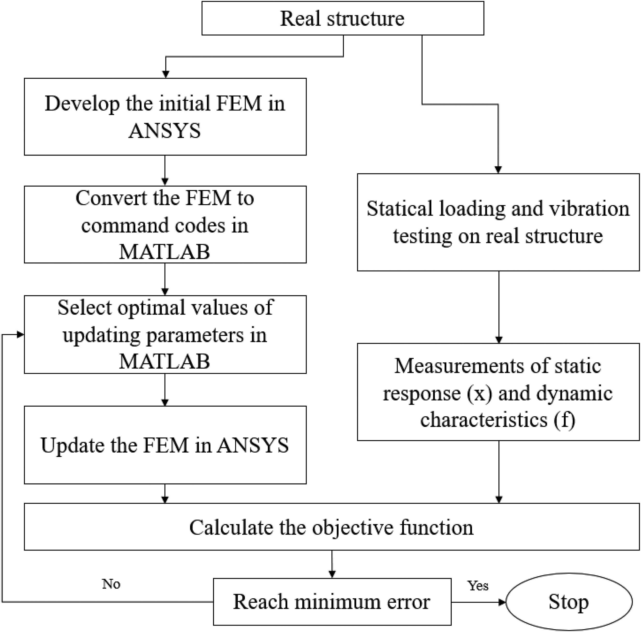
A novel approach for finite element model updating using MATLAB and Ansys.

Initial model development: Construct a baseline FE representation of the HFSS.

Parameter selection: Identify influential updating variables (θ) through sensitivity analysis.

Experimental validation: Acquire measured structural responses, including pole displacements and natural frequencies.

Objective function: Define a performance metric quantifying discrepancies between numerical and experimental results.

Optimization phase: Employ computational algorithms to iteratively minimize the objective function.

Model verification: Assess the calibrated model's accuracy and physical consistency.

The approach ensures systematic refinement of FE predictions to match real-world behavior, enhancing reliability for subsequent analyses.

Local stiffness of semi-rigid joints and initial structural imperfections

Semi-rigid joints are critical components in spatial network structures, governing global stability and load-bearing capacity. The fixity factor (ranging from 0 for pinned to 1 for rigid connections) quantifies their rotational stiffness and deformation capacity. This study adopts semi-rigid joint modeling, replacing idealized rigid assumptions to accurately capture nonlinear mechanical behavior. The initial stiffness S of semi-rigid joints is directly linked to Young's modulus E, enabling dynamic updates of the stiffness matrix in numerical simulations. By calibrating E and S, the global stiffness matrix can be adjusted to precisely replicate moment-rotation (M-Φ) curves. Experiments and numerical analyses demonstrate that initial joint stiffness significantly impacts critical buckling loads. This study combines experimental calibration (M-Φ) with advanced FE modeling to address semi-rigid joint nonlinearity.

Spatial network structures are highly sensitive to geometric imperfections, particularly in flexible systems like HFSSs. Building codes mandate perpendicularity deviations below 1/500H (where H is the structure height) and initial pole curvature under 1/1000L (where L is the pole length). Benchmarking against building codes and empirical data ensures theoretical rigor. To simulate real-world imperfections, this study employs the first-order buckling mode as the initial defect distribution, integrated into the FEM via modal superposition. Quantifies defect impacts using buckling modes, aligns with engineering practice and enhances predictions.

Selection of updating parameters

The selection of updating parameters in the FEM updating critically influences the accuracy and reliability of the calibrated model. Parameters must be chosen based on their physical significance and sensitivity to the structural responses of interest, while ensuring identifiability to avoid over-parameterization. Guided by prior studies and the structural characteristics of the system under investigation, the following parameters were selected for updating such as initial stiffness of semi-rigid joints, Young's modulus (E), Poisson's ratio (ν), real constant of the diagonal brace, and density (ρ). The initial values and bounds for these parameters are summarized in Table 1. The baseline material properties were set to E = 210 GPa, ν = 0.3, and ρ = 7850 kg/m³, with Rayleigh damping coefficients α₁ = 0.01998 and α₂ = 1.9998 (derived from a nominal damping ratio ζ = 0.01).

Table 1.

Material and geometric parameters for FEM optimization.

Components		Standing poles and horizontal ledgers	Diagonal brace	Joints
Geometric dimension	OD (mm)	48	48	$\sim$
	Thickness (mm)	3.2	2.5	$\sim$
	ACS (mm²)	450	357	$\sim$
Initial stiffness (kN $\cdot$ m/rad)	Initial value	$\sim$	$\sim$	65
Initial stiffness (kN $\cdot$ m/rad)	Range	$\sim$	$\sim$	[58.5, 71.5]
Young's Modulus E (GPa)	Initial value	206	206	$\sim$
Young's Modulus E (GPa)	Range	[185.4, 226.6]	$\sim$	$\sim$
Possion ratio $ν$	Initial value	0.3	0.3	$\sim$
Possion ratio $ν$	Range	[0.27, 0.33]	$\sim$	$\sim$
Real constant r (mm²)	Initial value	450	357	$\sim$
Real constant r (mm²)	Range	[420, 480]	[320, 380]	$\sim$
Density $ρ$ (kg/m³)	Initial value	7800	7800	$\sim$
Density $ρ$ (kg/m³)	Range	[7020, 8580]	$\sim$	$\sim$

OD: outer diameter; ACS: area of cross section; FEM: finite element model.

A systematic sensitivity analysis was conducted to quantify the influence of each parameter on the structural responses. Each parameter was perturbed by ±10%, and the resulting changes in the following responses were evaluated: The first seven natural frequencies of the structure and 20 nodal displacements (D₁–D₂₀) on the standing poles, as shown in Figure 3. The sensitivity results, as shown in Figure 4(a), revealed that displacements D₁, D₄, D₆, D₁₀, D₁₁, D₁₃, D₁₅, D₁₇, and D₁₈ exhibited negligible sensitivity (normalized sensitivity index < 2) and were thus excluded from subsequent updating to improve computational efficiency. For frequencies, the scaled sensitivities, as shown in Figure 4(b), demonstrated that the first three modes were most sensitive to the selected parameters, with all sensitivities being positive—consistent with the expected trend that increased stiffness elevates natural frequencies. Consequently, the following responses were retained for updating, including displacements: D₂, D₃, D₅, D₇, D₈, D₉, D₁₂, D₁₄, D₁₆, D₁₉, D₂₀, and frequencies: First three natural modes.

Figure 3.

Distribution of sensor locations.

Figure 4.

(a) Sensitivity analysis for displacements; (b) sensitivity analysis for frequencies.

This selection ensures a balance between information richness (prioritizing highly sensitive responses) and parameter identifiability (avoiding redundancy). The exclusion of low-sensitivity measurements aligns with the principles of parsimony in model calibration, while the retained responses capture the dominant properties of the structure.

Definition of the objective function

To optimize the model parameters, an iterative updating procedure is employed. Initially, suitable starting values are assigned to the parameters, which are then refined through an optimization process. A well-defined objective function is essential to guide this parameter updating. Experimental data, including structural responses such as accelerations and displacements, are collected for validation. The objective function is formulated based on discrepancies in both displacement and frequency responses, as expressed in Equation 1:

m i n R (θ) = \min (\sum_{i = 1}^{m} {(\frac{x_{i}^{'} - x_{i}}{x_{i}})}^{2} + \sum_{j = 1}^{n} {(\frac{f_{j}^{'} - f_{j}}{f_{j}})}^{2})

(1)

where x_i and x_i′ denote the measured and computed displacements, respectively; f_j and f_j′ represent the measured and computed frequencies, respectively. This formulation ensures a balanced minimization of relative errors in both displacement and frequency domains, enhancing the model's fidelity to experimental observations.

Experiment setup

The experimental investigation focuses on a five-story HFSS constructed from steel pipes, comprising vertical standing poles, horizontal ledgers, and diagonal braces bolted at the joints to form a rigid truss structure, as shown in Figure 5. The system has a total height of 8 m, with a lift height of 1.5 m per level. The overall dimensions of the structure are approximately 5 m in length and 4 m in width, with a transverse spacing of 1.2 m and a longitudinal spacing of 0.9 m between adjacent standing poles. Static loading was applied to the structure using four hydraulic jacks mounted on a reaction frame. Concentrated loads were imposed on the top of the structure and evenly distributed to each standing pole via load distribution beams. To assess localized behavior, only two of the four jacks were activated in certain loading phases. The loading protocol involved incremental force application, with each step introducing an additional 10 kN. As the load approached the structure's estimated ultimate capacity, the increment size was reduced to closely monitor nonlinear behavior. Loading progression was governed by real-time strain and displacement measurements from critical standing poles. A new load step was initiated only after stabilization of the measured responses. The ultimate bearing capacity was determined when displacements continued to increase despite unloading, indicating structural failure.

Figure 5.

The full-size configuration of the high-formwork support system.

To evaluate the dynamic characteristics of the structure, an electrodynamic shaker was employed to generate controlled impact excitations. The applied impact forces were precisely monitored using a high-precision load cell, while the structural response was captured through triaxial accelerometers positioned along the X, Y, and Z axes, as shown in Figure 6. This multi-directional sensor configuration enabled comprehensive modal analysis of the structural system. The experimental data acquisition system recorded both the excitation forces and corresponding acceleration responses with a sampling frequency range of 0––100 Hz, as shown in Figure 7. Structural frequencies were measured at multiple loading stages to account for stiffness variations induced by progressive loading. The evolution of the stiffness matrix throughout the loading process resulted in measurable shifts in the structure's natural frequencies at each load increment.

Figure 6.

Placement strategy for acceleration transducers.

Figure 7.

(a) Measured impact force time-history; (b) acceleration time-history at monitoring points A1 and A2.

Displacement meters, total-station instruments, a leveling instrument, and a 3D laser scanner were used to measure the displacements of standing poles. The laser scanning methodology, which provided high-resolution displacement measurements of the standing poles, followed the established protocol detailed in.⁵¹ This comprehensive instrumentation strategy ensured robust quantification of both static and dynamic structural behavior throughout the testing protocol.

Frequency and mode shapes

The structural frequencies and corresponding mode shapes were extracted from acceleration measurements using power spectral density (PSD) analysis, a well-established technique for modal parameter identification that has been extensively validated in previous studies.^52,53 The PSD analysis of the acceleration time histories, as shown in Figure 8(a), was performed. The resulting spectrum, as displayed in Figure 8(b), reveals distinct peaks, which correspond to the structure's natural frequencies.

Figure 8.

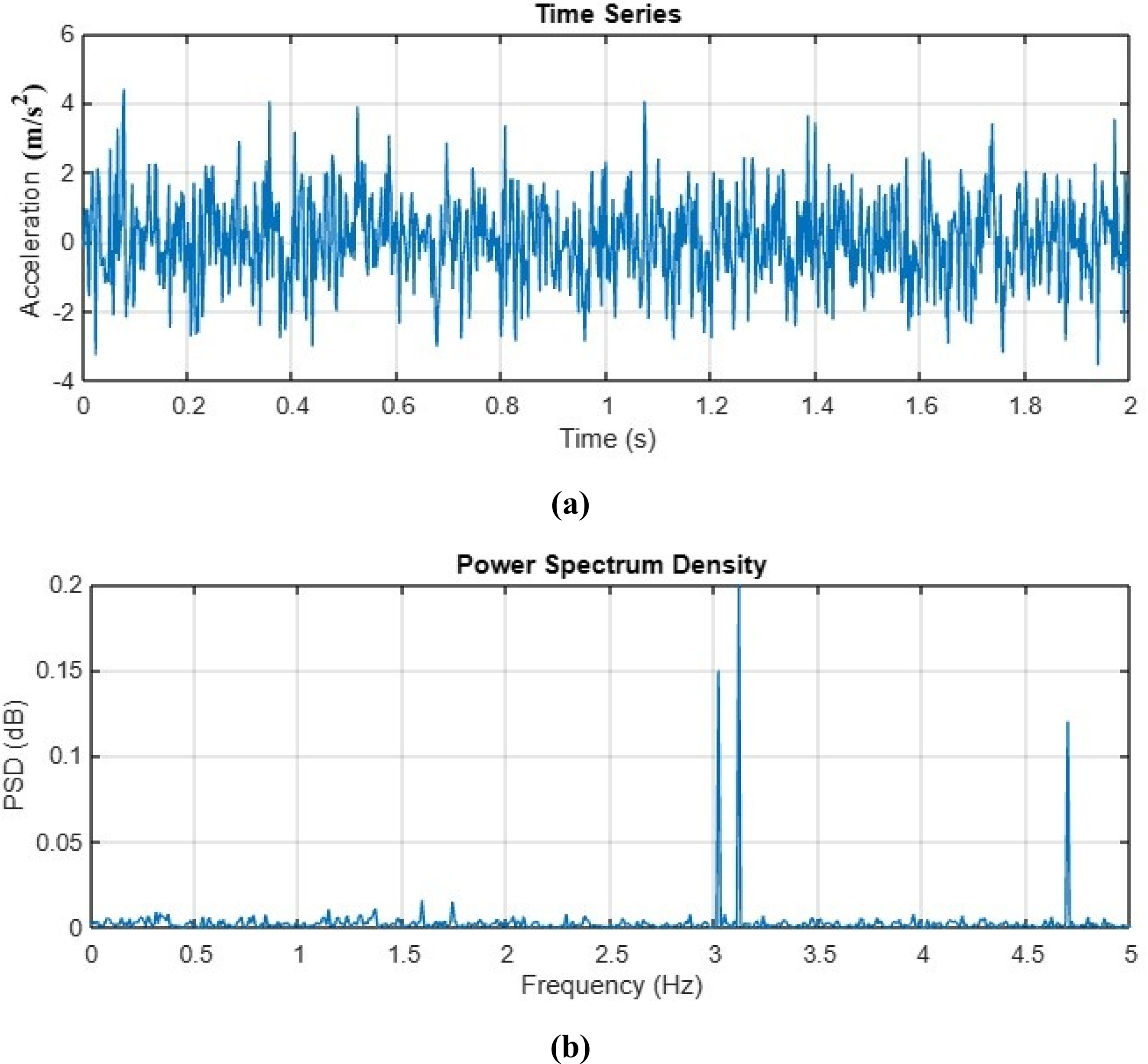
(a) Acceleration temporal response, (b) power spectral density (PSD) frequency analysis.

The PSD exhibits significant variation near resonant frequencies, with pronounced peaks indicating fundamental modes. Our analysis identified three dominant vibration modes at 3.024, 3.152, and 4.826 Hz, representing the structure's primary dynamic characteristics. The PSD-based method proved particularly effective for this structural configuration, as evidenced by the well-defined spectral peaks and consistent mode shape patterns across multiple measurement points.

Simulation of abnormal working conditions

The structural performance was evaluated under both normal and abnormal working conditions to validate the proposed classification approach. Two primary abnormal conditions were investigated: Local instability and global instability states. Local instability occurs when concentrated loads are applied to specific standing poles, causing localized components to reach their ultimate bearing capacity while the overall structure maintains partial integrity. This condition is characterized by reduced local stiffness without complete structural collapse. In contrast, global instability represents complete structural failure, where the entire system reaches its ultimate load-bearing capacity and loses all functionality.

The identification of these abnormal conditions was achieved through analysis of the structure's dynamic characteristics rather than complex FE simulations. Both local and global instability states exhibit distinct deviations from normal conditions in terms of natural frequencies and mode shapes. As shown in Figure 9, the first four mode shapes demonstrate significant differences between normal operation and local instability conditions. While the normal state maintains typical bending and torsional modes, the local instability condition reveals noticeable deviations due to stiffness reduction. Furthermore, time-domain analysis of acceleration responses provides additional evidence, with clear divergence observed between normal and abnormal states as shown in Figure 10.

Figure 9.

Initial four modal shapes of the high-formwork support system (HFSS) under both operational conditions and partial buckling scenarios.

Figure 10.

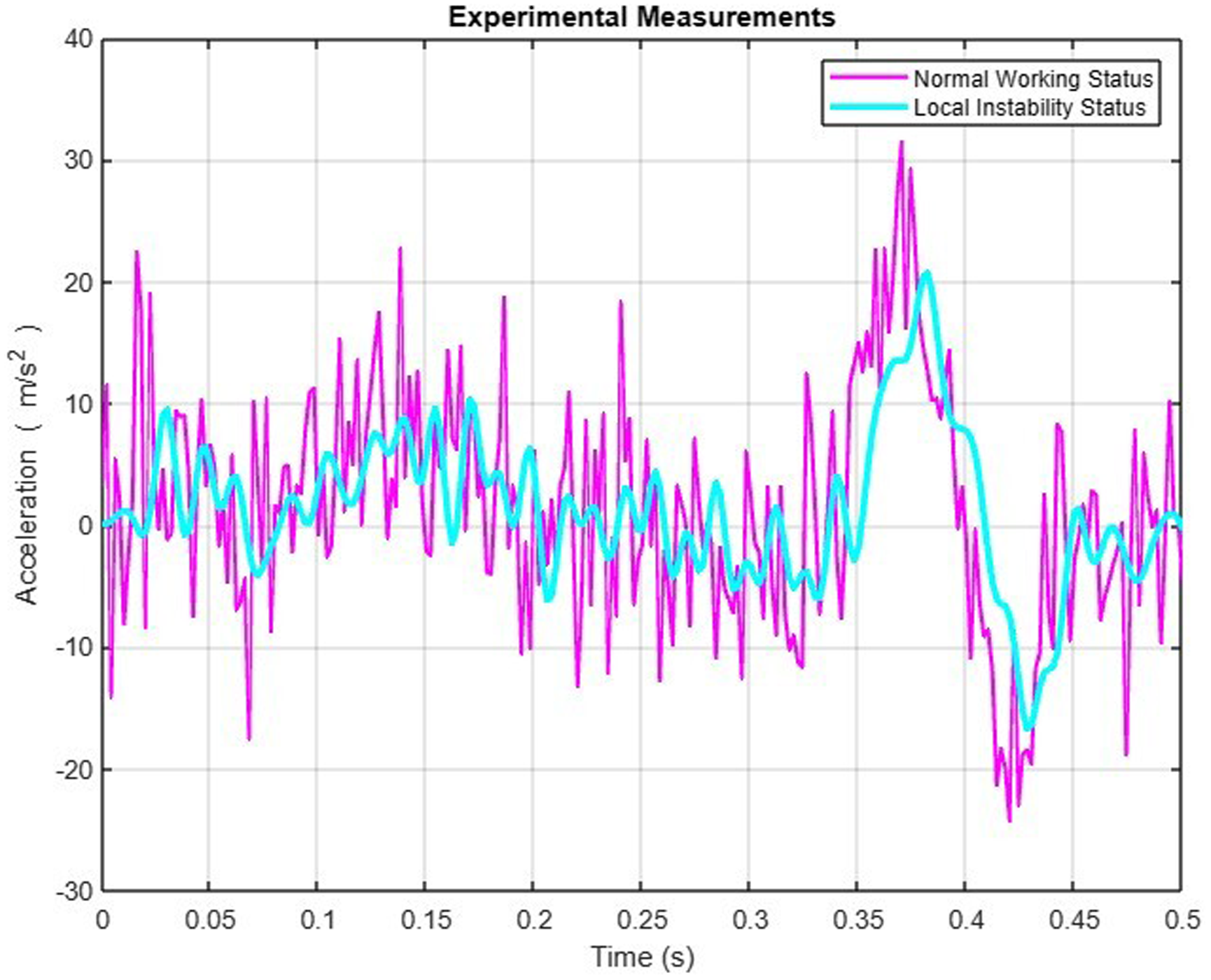
Comparative analysis of acceleration time-history measurements between standard operating conditions and localized instability scenarios in the high-formwork support system.

The experimental investigation employed a full-scale HFSS subjected to controlled loading scenarios. Initial tests applied localized forces to induce and measure local instability conditions. After recording these measurements, the damaged standing poles were replaced to restore structural integrity. Subsequently, progressively increasing loads were applied until global instability was achieved, allowing comprehensive data collection across the complete range of structural states. This systematic approach enabled precise characterization of the transition from normal operation through partial damage to complete structural failure.

Measurement errors

Noise removal using filtering

Due to structural non-stationarity, dynamic variations, and the effects of sensor sensitivity and signal transmission, the acquired acceleration data often contain noise, outliers, and anomalies. Such distortions can significantly compromise signal integrity. Hence, the normalization procedure linearly maps the acceleration of different sensors to the same scale between −1 and 1 to diminish the scale effect. Then, appropriate filtering techniques are essential for effective data preprocessing. In this study, a Butterworth filter is employed for noise suppression, characterized by its flat frequency response in the passband. The transfer function of the filter is given in Equation 2.

| H (ω) |^{2} = \frac{1}{1 + {(\frac{ω}{ω_{c}})}^{2 n}}

(2)

where ω is the input frequency value, corresponding to the time step in energy consumption. ω_c is the corresponding cutoff frequency, and n is the order of the filter.

The selection of the Butterworth filter's order involves a trade-off between noise attenuation and computational efficiency. A second-order filter is widely adopted in practice due to its optimal balance between smoothing performance and computational simplicity. Accordingly, this study employs a second-order Butterworth filter for signal processing. The difference between the original signal and the refined signal is shown in Figure 11.

Figure 11.

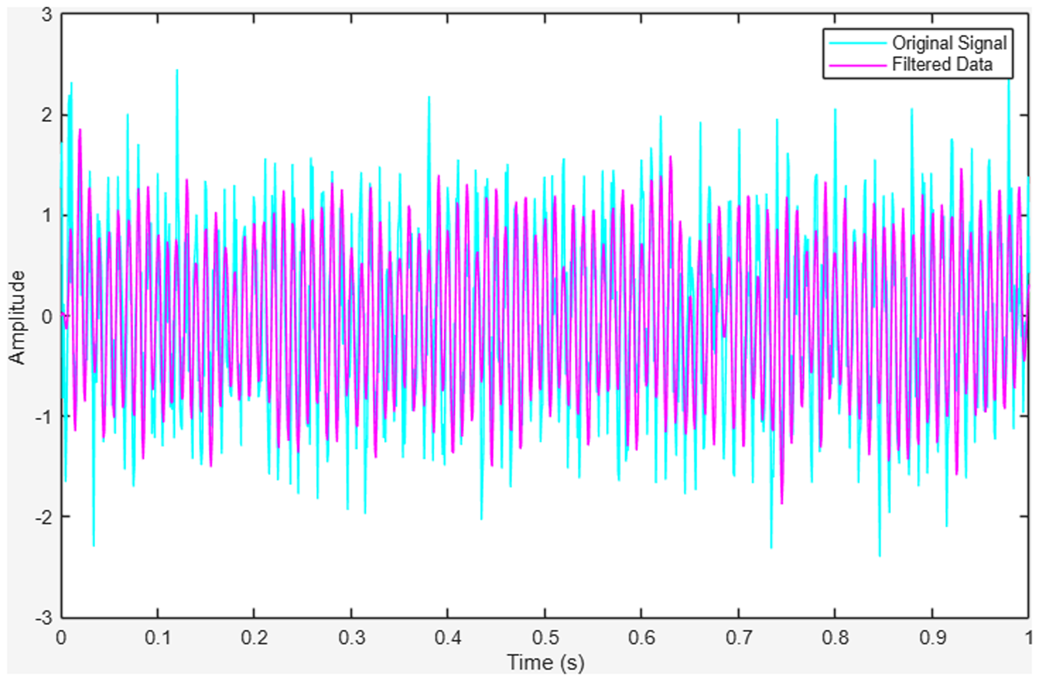
The original signal and the filtered signal.

Moreover, to rigorously evaluate the robustness of the proposed filter, the study incorporated Gaussian noise at varying intensities into the input signals. Specifically, noise-to-signal ratios of 5%, 10%, and 15% were introduced to simulate real-world signal degradation. The filtering performance was then quantitatively assessed using signal-to-noise ratio (SNR), mean squared error (MSE), and peak SNR (PSNR), as shown in Table 2.

Table 2.

Quantitative assessment for the filter.

Noise level	SNR(original)(db)	SNR(filtered)(dB)	MSE	PSNR
5%	23.1	32.5	0.015	38.2
10%	17.8	28.3	0.042	33.8
15%	14.2	24.7	0.089	29.5

SNR: signal-to-noise ratio; PSNR: peak signal-to-noise ratio; MSE: mean squared error.

The correlation of measurements

During the FEM updating for the structure, it is observed that the measurements, such as displacements of standing poles, are correlated. To account for the correlation between measurements in the FEM updating process, the covariance matrix was decomposed. This decomposition transforms the correlated displacement measurements into a linear combination of independent stochastic variables. Then, the displacement measurement vector $x_{u}$ is defined in Equation 3.

x_{u} = x_{u 0} + \sum_{i = 1}^{m} ξ_{i} \sqrt{λ_{i}} Φ_{i}

(3)

where $x_{u 0} = [x_{10}, x_{20}, \dots, x_{m 0}]$ is the mean of the displacement measurement vector. $λ_{i}$ and $Φ_{i}$ indicate the eigenvalues and eigenvectors of the covariance matrix $C o v (x_{u}, x_{u})$ , respectively. $ξ_{i}$ denotes a set of independent stochastic variables having zero mean and one variance.

Comparative analysis of optimization algorithms

To minimize the proposed objective function, four optimization algorithms were evaluated: GBO, GA, GWO, and a hybrid GA-PSO. The statistical results of the FEMU using these algorithms are presented in Table 3.

Table 3.

Comparative performance of optimization algorithms in FEMU.

Mode		1	2	3	4
Measured frequencies (Hz)		3.024	3.152	4.826	5.397
GA	mean f (Hz)	3.139	3.272	5.009	5.602
GA	std f	1.474E-02	3.081E-02	2.461E-02	2.783E-02
GA-PSO	mean f (Hz)	3.028	3.158	4.831	5.402
GA-PSO	std f	8.726 E-03	1.142E-02	1.038E-02	1.254E-02
GBO	mean f (Hz)	3.211	3.347	5.125	5.732
GBO	std f	2.845E-02	3.675E-02	3.724E-02	3.897E-02
GWO	mean f (Hz)	3.236	3.373	5.164	5.775
GWO	std f	2.547E-02	3.112E-02	5.012E-02	3.962E-02

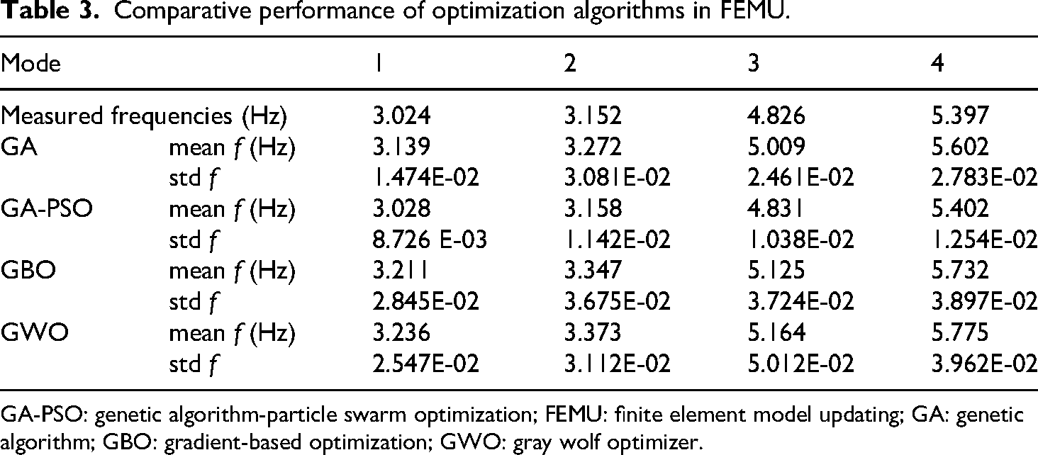
GA-PSO: genetic algorithm-particle swarm optimization; FEMU: finite element model updating; GA: genetic algorithm; GBO: gradient-based optimization; GWO: gray wolf optimizer.

Among the tested methods, the hybrid GA-PSO demonstrated superior performance, yielding the most accurate and consistent results. Specifically, the first four computed frequencies and corresponding mode shapes exhibited complete agreement with the experimentally measured modal data. While GBO and GWO provided satisfactory displacement predictions for standing poles, their correlation with experimental frequencies remained suboptimal. Additionally, GA exhibited notable limitations, including premature convergence and a tendency to settle in local optima. Overall, the GA-PSO algorithm proved to be the most efficient and reliable for FEMU, as evidenced by its convergence behavior, as shown in Figure 12.

Figure 12.

Objective function convergence profiles among four optimization algorithms.

The GA-PSO approach combines the strengths of both optimization methods through an integrated two-stage process. Initially, the GA generates and evaluates an initial population, sorting solutions by fitness value. The most promising candidates from this GA phase are then passed to the particle swarm optimizer, where they initialize both the personal best positions and global best position for the swarm. This information transfer ensures PSO begins its search in promising regions of the solution space. The algorithm iteratively refines solutions through this collaborative process until meeting either the convergence thresholds or the prescribed maximum number of iterations.

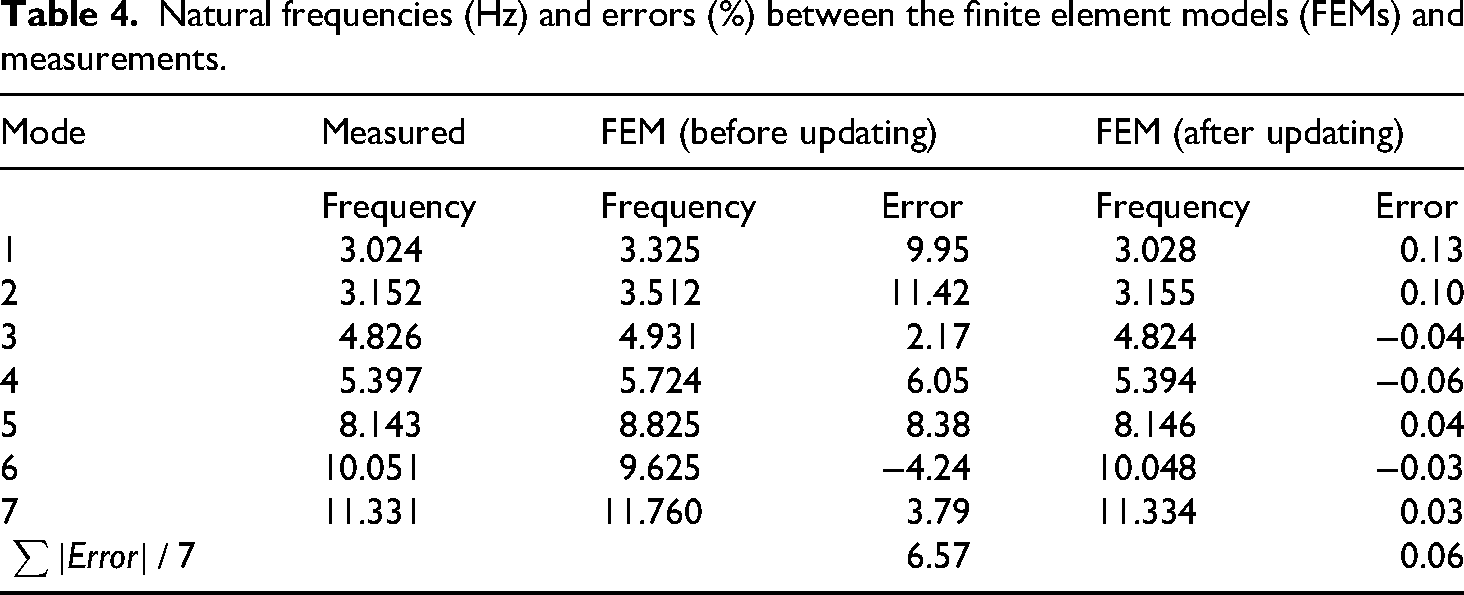
Figure 13 presents a comparative analysis between the predicted modes from the GA-PSO optimized FEM and experimental modal test results. The modal assurance criterion (MAC) matrix demonstrates excellent correlation, with strong diagonal dominance persisting through the eighth mode. Table 4 summarizes the corresponding frequency comparisons between the optimized FEM, nominal model, and experimental measurements. The MAC values, which range from 0 (no correlation) to 1 (perfect correlation), consistently approach unity for corresponding mode pairs. This indicates strong agreement between the predicted and experimental mode shapes, validating the optimization results. The close frequency matching shown in Table 3 further confirms the model's accuracy.

Figure 13.

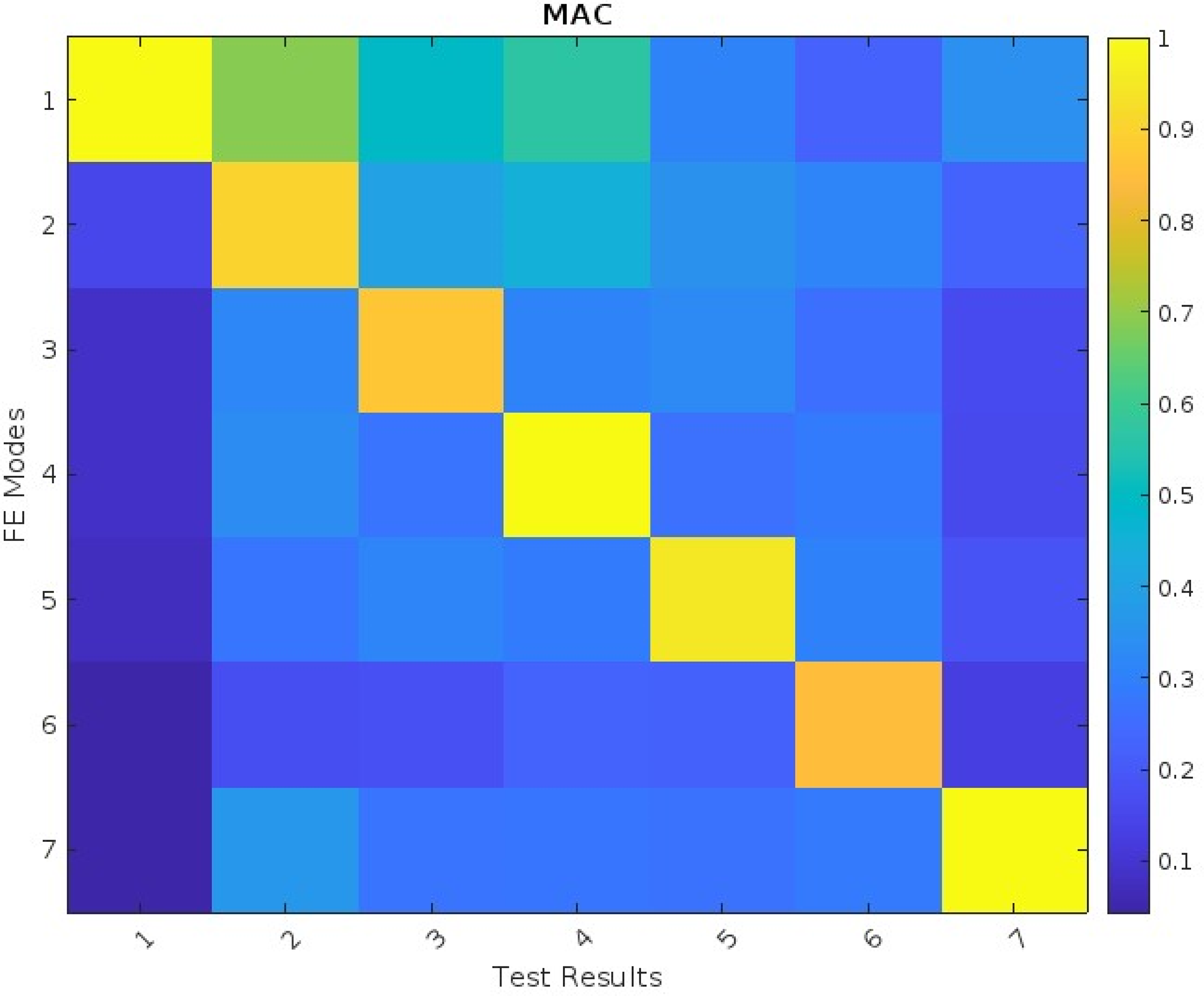
Modal assurance criterion (MAC) results following parameter updating.

Table 4.

Natural frequencies (Hz) and errors (%) between the finite element models (FEMs) and measurements.

Mode	Measured	FEM (before updating)		FEM (after updating)
	Frequency	Frequency	Error	Frequency	Error
1	3.024	3.325	9.95	3.028	0.13
2	3.152	3.512	11.42	3.155	0.10
3	4.826	4.931	2.17	4.824	−0.04
4	5.397	5.724	6.05	5.394	−0.06
5	8.143	8.825	8.38	8.146	0.04
6	10.051	9.625	−4.24	10.048	−0.03
7	11.331	11.760	3.79	11.334	0.03
$\sum \| E r r o r \| / 7$			6.57		0.06

RNN-LSTM model training and experimental validation

RNN-LSTM architecture

Recurrent neural networks (RNNs) represent a class of artificial neural networks characterized by directed cyclic connections, enabling the retention of temporal information and effectively serving as a form of memory. While RNNs excel at modeling sequential data, their conventional architectures suffer from a critical limitation: The vanishing gradient problem, which impedes their ability to capture long-range dependencies in complex datasets. To address this challenge, Long Short-Term Memory (LSTM) networks—a specialized variant of RNNs—have been developed. LSTMs incorporate memory cells governed by three adaptive gating mechanisms: The input gate, forget gate, and output gate (Figure. 8). These gates regulate information flow through sigmoid activation functions, enabling selective retention or discarding of temporal features.

By integrating the temporal modeling capabilities of RNNs with the memory retention mechanisms of LSTMs, the hybrid RNN-LSTM framework achieves superior performance in capturing nonlinear, high-dimensional temporal patterns (Figure. 10). Training the RNN-LSTM model involves iterative optimization of weights and biases via backpropagation through time, minimizing prediction errors through gradient-based learning. This adaptive learning process allows the model to refine its representations continuously, enhancing its predictive accuracy as it processes new data.

RNN-LSTM model training

This section presents the methodology for generating training data from FEMs and describes the RNN-LSTM learning process. To systematically evaluate the impact of model fidelity on predictive performance, we employ two distinct datasets for network training: (1) Conventional nominal FEM outputs and (2) optimized FEM results (as developed inthe “FEM calibration” section). This comparative approach enables quantitative assessment of how enhanced FEM accuracy influences structural state forecasting capabilities.

The training dataset was generated using the optimized FE formulation detailed in the “FEM calibration” section. The fundamental dynamics are governed by Equation 4, which serves as the physical basis for all simulated training scenarios.

M (ρ) A + C (K, M, α_{1}, α_{2}) V + K (E, I) U = F

(4)

C = α_{1} M + α_{2} K

where U, V, and A are the displacement, velocity, and acceleration vector, respectively. K, C, and M represent stiffness matrices of the structure, damping, and global mass that relate to the model parameters of elasticity modulus E, damping $α_{1}, α_{2}$ , and density $ρ$ . The displacements of the standing pole and structural frequencies used for RNN-LSTM learning were simulated for arbitrary load cases by using Algorithm 1. The status labels Y were the categories of the working statuses of the structure in this work.

Algorithm 1: Finite element model data generation algorithm
Input: Number of load cases n and upper (up) and lower (lo) statistical bounds for each quantity
Output: n displacements and n number of labeled acceleration vectors
1. for i = 1:n do
2. define status y according to FE model $\to Y$
3. sample E $\to K = K (E)$
4. Solve $K X = F$
5. return displacement $X$
6. sample $ρ \to M = M (ρ)$
7. Solve $M A + K X + C V = F$
8. return $A a n d Y$
End

Algorithm 1: FEM data production algorithm

T r a i n_{s e t} = {(F_{1}, U_{1}, Y_{1}), (F_{2}, U_{2}, Y_{2}), \dots, (F_{n}, U_{n}, Y_{n})}

To systematically evaluate the impact of model fidelity on predictive performance, we conducted parallel training using both nominal and optimized FEM-generated datasets. The comparative analysis reveals significant improvements in prediction accuracy when employing the optimized FE formulation (the “FEM calibration” section). All FE simulations were performed using ANSYS (v2021R1) on a high-performance computing node (Intel i7–8700, 64GB Random Access Memory (RAM)) with consistent convergence criteria.

To rigorously assess model robustness, we introduced controlled Gaussian noise perturbations to the optimized dataset at three distinct noise-to-signal ratios (5%, 10%, and 15%). This experimental design enables quantitative evaluation of the RNN-LSTM's noise immunity while maintaining the physical consistency of the underlying FE solutions. The complete dataset characteristics are detailed in Table 5.

Table 5.

FE produced data for the RNN-LSTM.

Case	FEM	Number of cases
NWS	Nominal	1000
	Optimal	1000
	Optimal with 5% error	300
	Optimal with 10% error	300
	Optimal with 15% error	300
LIS	Nominal	1000
	Optimal	1000
	Optimal with 5% error	300
	Optimal with 10% error	300
	Optimal with 15% error	300
FIS	Nominal	1000
	Optimal	1000
	Optimal with 5% error	300
	Optimal with 10% error	300
	Optimal with 15% error	300

NWS: normal working status; LIS: local instability status; FIS: fully instability status; RNN-LSTM: recurrent neural network long short-term memory; FEM: finite element model; FE: finite element.

The comparative training results are presented in Table 6. The RNN-LSTM model trained on optimized FEM data achieved the highest prediction accuracy (95.8%), demonstrating its effectiveness in capturing the essential characteristics of the structural system. In contrast, the model trained using nominal FEM data showed substantially lower performance (71.3% accuracy), confirming that the quality of training data significantly impacts model effectiveness. To evaluate robustness, we introduced Gaussian noise to the optimal dataset at varying intensities (5%, 10%, and 15% NSR). The model maintained strong performance with accuracies of 89.9%, 83.6%, and 76.9% respectively, indicating remarkable tolerance to input data imperfections. These results collectively demonstrate that while optimized FEM data enhances prediction accuracy, the proposed RNN-LSTM architecture maintains robust performance even with noisy input data.

Table 6.

Model training performance.

	Number of learning cases	Mean learning accuracy
Nominal finite element model (FEM) data	3000	71.3%
Optimal FEM data	3000	95.8%
Optimal FEM data with 5% error	900	89.9%
Optimal FEM data with 10% error	900	83.6%
Optimal FEM data with 15% error	900	76.9%

The RNN-LSTM model was successfully trained using the datasets, as illustrated in Figure 14 and detailed in Table 7. The training performance, quantified by mean classification accuracy for each structural state, is presented in Table 8. Notably, the model achieved classification accuracies exceeding 80% for all three structural states when trained on optimized FEM data. Furthermore, the model demonstrated robust performance even when trained on noise-contaminated data, maintaining satisfactory classification accuracy across all structural states. These results underscore both the model's strong learning capability and its practical applicability in real-world scenarios where measurement noise is inevitable. The training progress is shown in Figure 15.

Figure 14.

The proposed recurrent neural network long short-term memory (RNN-LSTM) classifier architecture.

Figure 15.

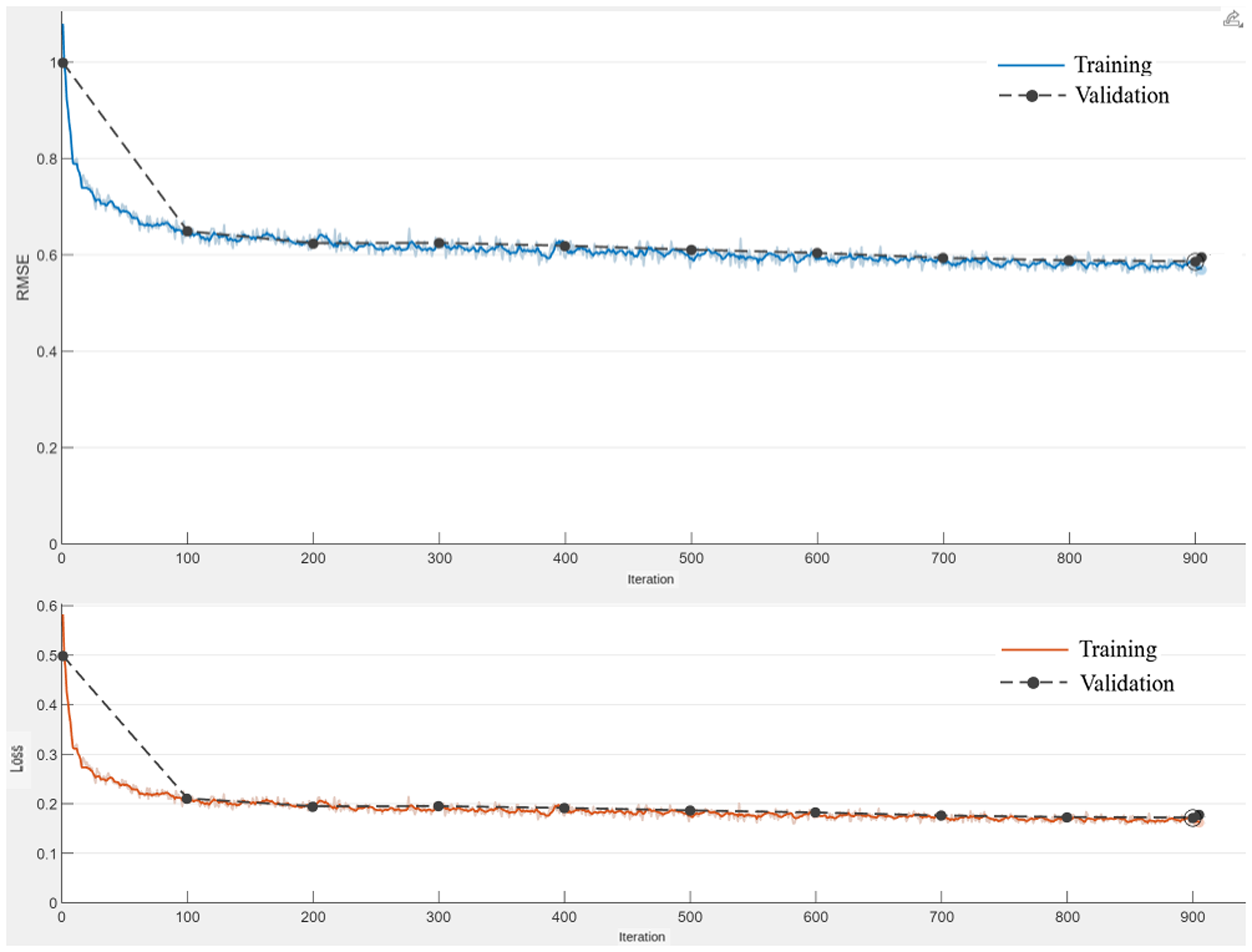
Training accuracy and loss trajectories of the recurrent neural network long short-term memory (RNN-LSTM) model.

Table 7.

The formation of the proposed RNN-LSTM model.

Hyperparameter	Specification
Network type	Bidirectional LSTM
Activation	Tanh (recurrent), Softmax (output)
Loss function	Categorical cross-entropy
Optimizer	Adam with gradient clipping
Recurrent dropout	0.2
Validation split	0.2
Learning rate	0.001

RNN-LSTM: recurrent neural network long short-term memory; LSTM: long short-term memory.

Table 8.

The learning and validation results for RNN-LSTM model.

Data	Case	NWS	LIS	FIS
Optimum FEM data	Mean learning accuracy	98.3%	94.7%	96.2%
Optimum FEM data	Mean validation accuracy	94.1%	93.8%	92.6%
Optimum FEM data with 5% error	Mean learning accuracy	88.9%	86.3%	89.1%
Optimum FEM data with 5% error	Mean validation accuracy	85.4%	84.7%	87.5%
Optimum FEM data with 10% error	Mean learning accuracy	84.3%	82.1%	83.8%
Optimum FEM data with 10% error	Mean validation accuracy	80.7%	81.4%	80.5%
Optimum FEM data with 15% error	Mean learning accuracy	78.9%	75.3%	76.8%
Optimum FEM data with 15% error	Mean validation accuracy	76.3%	73.2%	74.9%

RNN-LSTM: recurrent neural network long short-term memory; FEM: finite element model; FIS: fully instability status; NWS: normal working status; LIS: local instability status.

Experimental validation of the trained RNN-LSTM model

The experimental validation was conducted using a dataset of 300 field measurements (100 per structural state) to evaluate the predictive performance of the trained RNN-LSTM model. For comparative analysis, we simultaneously tested a CNN model under identical conditions. Figure 16 presents the classification probabilities generated by both models across all structural states. The visualization clearly demonstrates the RNN-LSTM's superior performance in several key aspects: (1) More distinct separation of prediction probabilities between different structural states, (2) greater consistency in correctly identifying normal operating conditions (top panels), and (3) significantly improved detection capability for both local (middle panels) and global instability (bottom panels) compared to the CNN baseline.

Figure 16.

(a) Experimental input predictions from networks trained using optimized finite element model (FEM) data; (b) experimental input predictions from networks trained using baseline FEM data.

The confusion matrix in Figure 17 demonstrates the RNN-LSTM model's classification performance, where diagonal cells show correct predictions (with percentages) and off-diagonal cells indicate misclassifications. Classification accuracy and error rates are in the rightmost columns, while recall and false discovery rates are displayed in the bottom rows. The results demonstrate that the RNN-LSTM model trained with optimal FEM data achieves an overall accuracy of 98.5%, significantly outperforming the model trained with nominal FEM data (79.5%). Furthermore, the RNN-LSTM maintains robust performance under noisy conditions, delivering accuracies of 91.5%, 85.3%, and 76.9% for datasets corrupted with 5%, 10%, and 15% additive Gaussian noise, respectively.

Figure 17.

Classification performance matrix of RNN-LSTM model (a) trained with refined FEM dataset; (b) trained with unmodified FEM dataset; (c) trained on data with 5% additive noise; (d) trained on data with 10% additive noise; (e) trained on data with 15% additive noise. RNN-LSTM: recurrent neural network long short-term memory; FEM: finite element model.

As illustrated in Figure 18, the CNN achieves strong performance (96% overall accuracy) when trained on optimal FEM data. However, its effectiveness diminishes with nominal FEM data (78% accuracy) and further declines when handling noisy data. Specifically, the model attains accuracies of 83.7%, 75.4%, and 61.2% for datasets contaminated with 5%, 10%, and 15% additive Gaussian noise, respectively.

Figure 18.

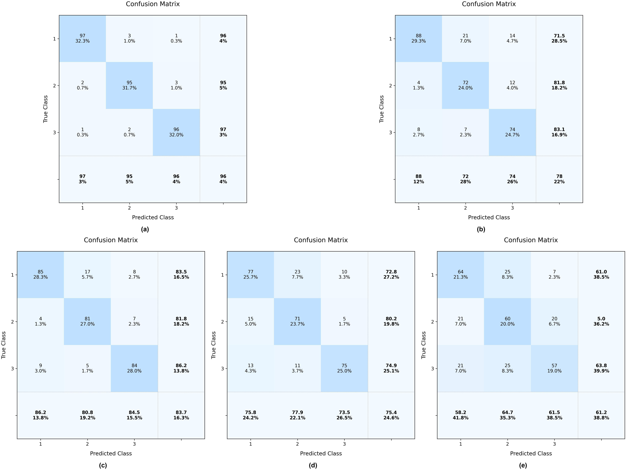
Classification performance matrix of CNN model (a) trained with refined FEM dataset; (b) trained with unmodified FEM dataset; (c) trained on data with 5% additive noise; (d) trained on data with 10% additive noise; (e) trained on data with 15% additive noise. FEM: finite element model; CNN: convolutional neural network.

The development process of the RAG model

The construction of the KG

In this study, the bottom-up approach was employed for the development of the KG, as shown in Figure 19. Firstly, the data is obtained from data sources including guidelines, case studies, and online relevant sources. Next, data cleaning by using a deep-learning language error correction model was conducted to enhance the quality of the KG. The research utilized natural language processing techniques for named entity recognition (NER) to extract entities and their connections.

Figure 19.

Development workflow diagram of the knowledge graph.

The NER approach, enhanced with part-of-speech tagging, systematically extracts subjects and objects as entities while categorizing verbs as relational elements. This process involves three key phases: (1) Entity detection, (2) relationship extraction, and (3) attribute specification. Following these extraction steps, knowledge consolidation is performed through graph operations such as node duplication, consolidation, addition, and deletion. The structured output is then imported into Neo4j for storage. The completed KG serves as an external knowledge repository for further applications. Figure 20 shows the complete toolchain used for the KG development process.

Figure 20.

Development toolkit supporting end-to-end knowledge graph (KG) construction.

The RAG model

The RAG framework integrates three core components: (1) A knowledge base, (2) information retrieval systems, and (3) generative AI models. In the developed implementation, the model first queries a domain-specific KG—constructed from SHM guidelines and empirical case studies—to retrieve contextually relevant data. This KG functions as an on-demand semantic database, enabling the RAG system to produce technically grounded responses. Particularly for specialized domains like SHM, this architecture significantly enhances output reliability by leveraging structured, verifiable knowledge during the generation process.

The developed RAG architecture integrates GPT-4 with a structured KG through the LangChain framework. This implementation enables natural language queries to be automatically translated into Cypher query language via LangChain's processing pipeline. The system establishes a bidirectional connection between GPT-4 and the Neo4j graph database, where Cypher queries efficiently retrieve relevant entities and relationships from the KG. These structured results are subsequently incorporated into GPT-4's generation process to enhance response accuracy and technical reliability. The complete system workflow is illustrated in Figure 21.

Figure 21.

Retrieval-augmented generation (RAG) implementation workflow.

Verification of the developed RAG model

The assessment was performed by comparing the SHM reports generated by the developed RAG model and GPT-4 model based on the project summary. To comprehensively evaluate the structural condition of HFSSs, the final SHM report must systematically incorporate several critical components: Project specifications (including structural parameters and environmental conditions), clearly defined monitoring objectives, detailed descriptions of the monitoring methodology and instrumentation, collected monitoring data sets, and analytical results with conclusions. This established framework enables a rigorous comparative assessment of how effectively different models can generate pertinent SHM reports for HFSS structures when presented with specific project scenarios, with model performance being evaluated against multiple quantitative metrics.

The semantic similarity assessment employed two complementary metrics: Cosine similarity (range: 0–1) and Euclidean distance, computed using embedding vectors generated by both BERT⁵⁴ and OpenAI's models. Higher cosine similarity scores (approaching 1) and smaller Euclidean distances indicate greater semantic correspondence between compared elements.

The study implemented two established evaluation metrics: BLEU⁵⁵ and the ROUGE,⁵⁶ to quantitatively assess the semantic alignment between generated responses and reference reports. The BLEU metric evaluates n-gram overlap with human-authored texts, measuring linguistic accuracy and fluency, while ROUGE analyzes content coverage through longest common subsequences, determining key information retention.

The comparative analysis employed 38 case studies to benchmark model performance. As presented in Table 9, quantitative metrics reveal distinct capabilities: BLEU and ROUGE scores demonstrate lexical precision in key term retention, while cosine similarity and Euclidean distance metrics quantify semantic alignment with reference materials.

Table 9.

Quantitative metrics of the responses produced by the models.

		RAG	GPT-4
BLEU(Bi-gram)		0.055	0.038
BLEU(Uni-gram)		0.222	0.126
BERT	Cosine	0.874	0.845
	Euclidean	7.117	7.223
OpenAI	Cosine	0.622	0.634
	Euclidean	0.941	0.916
RougeL	Precision	0.050	0.030
	Recall	0.079	0.094
	F1	0.053	0.015
RougeLsum	Precision	0.066	0.041
	Recall	0.104	0.132
	F1	0.067	0.045
Rouge1	Precision	0.063	0.044
	Recall	0.103	0.122
	F1	0.074	0.056
Rouge2	Precision	0.008	0.003
	Recall	0.103	0.121
	F1	0.009	0.006

RAG: retrieval-augmented generation; AI: artificial intelligence.

The minimal variance in cosine similarity and Euclidean distance metrics across models suggests strong semantic alignment between generated responses and reference texts. However, the RAG model demonstrates superior performance in lexical precision, with BLEU and ROUGE-L scores exceeding GPT's outputs by 27.8% and 32.8%, respectively. This performance gap highlights RAG's domain-specific optimization, enabling more accurate SHM terminology usage compared to GPT's generic formulations.

The evaluation reveals a notable divergence in model capabilities: While the RAG model achieves superior BLEU (0.055 vs 0.038) and ROUGE (0.066 vs 0.041) scores (p < 0.05), GPT demonstrates higher cosine similarity (0.622 vs 0.634). This dichotomy stems from their fundamental architectures: GPT's extensive pretraining on heterogeneous corpora enables broad semantic understanding but limits domain-specific precision, whereas RAG's knowledge-augmented design optimizes technical accuracy in the SHM domain.

The verification analysis reveals distinct response patterns: The RAG framework consistently generates technically detailed outputs by leveraging domain-specific KG retrievals, whereas GPT produces more generic responses. While RAG demonstrates superior technical accuracy, its knowledge-graph dependency limits response variation, reflecting the fundamental trade-off between precision and diversity in knowledge-enhanced language models.

Conclusion

This study presents a DL framework for identifying working status in HFSSs, utilizing an RNN-LSTM architecture. The methodology comprises three key phases: (1) FEMU through optimization, (2) dataset generation from the calibrated FEM, and (3) RNN-LSTM network development. A full-scale HFSS structure was used to obtain experimental measurements that serve two purposes: FEM calibration and RNN-LSTM performance verification. During the FEM updating phase, four optimization algorithms—GBO, GA, hybrid GA-PSO, and GWO—were systematically evaluated. Benchmarking results demonstrated the superior performance of the GA-PSO hybrid algorithm in achieving optimal model convergence.

The dataset generated by the optimized FEM was employed to train the RNN-LSTM network. This FEM-derived training approach significantly reduces experimental resource requirements while ensuring data adequacy. Comparative analysis revealed that datasets from non-optimized FEM simulations proved insufficient for robust multiclass identification, underscoring the importance of the initial model updating phase. The RNN-LSTM architecture demonstrated superior performance to CNN when validated against experimental measurements, attributable to its multi-filter design that effectively captures critical temporal patterns and hierarchical features in the structural response data.

Moreover, this study proves the practical application of specialized LLMs in the SHM domain. By adopting LLMs tailored to domain-specific needs, the study described the auto-generation of the SHM report for the HFSS. The developed RAG model could significantly reduce the time and effort required for producing such SHM reports.

This study compared two representative DL architectures, CNNs and RNN-LSTMs. To further generalize and validate these findings, future research could explore a broader spectrum of models, including recent advancements in optimization and other DL paradigms. Moreover, this study categorized the working status of HFSSs into three types: Normal working status, local instability, and global instability. Future research will further expand this classification to include other critical status, such as differential settlement. Additionally, developing a real-time monitoring system and rigorously quantifying the uncertainty of predictions are critical next steps.

Table of acronyms

Acronym	Meaning
AE	Autoencoder
ANFIS	Adaptive Fuzzy Neuro Inference System
ANNs	Artificial Neural Networks
AI	Artificial Intelligence
AE	Autoencoder
ANFIS	Adaptive Fuzzy Neuro Inference System
ANNs	Artificial Neural Networks
AI	Artificial Intelligence
BNNs	Bayesian Neural Networks
BP	Back Propagation
CE	Cross Entropy
CNNs	Convolutional Neural Networks
DL	Deep Learning
FE	Finite Element
FEM	Finite Element Model
FEMU	Finite Element Model Updating
FIS	Fully Instability Status
GA	Genetic Algorithm
GANs	Generative Adversarial Networks
GBO	Gradient Based Optimizer
GPU	Graphics Processing Unit
GRNNs	General Regression Neural Networks
GSR	Gradient Search Rule
GWO	Grey Wolf Optimizer
HFSS	High-Formwork Support System
KGs	Knowledge Graphs
KL	Karhunen–Loève
LB	Lower Bound
LDA	Linear Discrimination Analysis
LEO	Local Escaping Operator
LIS	Local Instability Status
LLMs	Large Language Models
LSTM	Long Short-Term Memory
MAC	Modal Assurance Criterion
ML	Machine Learning
MLP	Multi-Layer Perception
MSE	Mean Squared Error
NWS	Normal Working Status
OD	Outer Diameter
PDF	Probability Distribution Function
PSD	Power Spectral Density
PSNR	Peak Signal to Noise Ratio
PSO	Particle Swarm Optimization
RAG	Retrieval Augmented Generation
RAM	Random Access Memory
RF	Random Forest
RNN	Recurrent Neural Network
SA	Simulated Annealing
SHM	Structural Health Monitoring
SNR	Signal to Noise Ratio
SVM	Support Vector Machine
UB	Upper Bound

Footnotes

Acknowledgements

The authors would like to thank Beijing University of Technology for its support through the research project. The authors would like to thank the China Industry Associations for providing research data. In addition, I would like to thank all practitioners who contributed to this project.

ORCID iD

Linlin Zhao

Author contributions

Conceptualization, L.Z.; methodology, L.Z.; software, R.Z.; validation, L.Z., J.M.; resources, L.Z., T.Z.; writing—original draftpreparation, L.Z.; writing—review and editing, C.H., L.L.; visualization, R.Z., T.Z.

Funding

The authors disclosed receipt of the following financial support for the research, authorship, and/or publication of this article: This work was supported by the Beijing University of Technology (Grant No. 047000513102) and the Natural Science Foundation of Beijing (Grant No. 8254038). The article processing charge was funded by these grants.

Declaration of conflicting interests

The authors declared no potential conflicts of interest with respect to the research, authorship, and/or publication of this article.

Data availability

The data can be provided upon request.

References

Mozaffari

Bruce

Clune

, et al. Digital design and fabrication of clay formwork for concrete casting. Autom. Constr 2023; 154: 1–13.

Reynolds

Zhang

Rasmussen

KJR

. Investigation of U-head rotational stiffness in formwork supporting scaffold systems. Eng. Struct 2017; 136: 1–11.

Zhao

Zhang

Mbachu

. Multi-sensor data fusion for 3D reconstruction of complex structures: A case study on a real high formwork project. Remote Sens 2023; 15: 1–31.

Yuan

Zargar

Chen

, et al. Machine learning for structural health monitoring: Challenges and opportunities. in Sensors and Smart Structures Technologies for Civil, Mechanical, and Aerospace Systems 2020, Online Only, California, United States; Society of Photo-Optical Instrumentation Engineer (SPIE). 2020.

Farrar

Worden

. Structural health monitoring a machine learning perspective. London.: Wiley, 2012.

Fink

Wang

Svensen

, et al. Potential, challenges and future directions for deep learning in prognostics and health management applications. Eng. Appl. Artif. Intell 2020; 92: 1–15.

Brozovsky

Labonnote

Vigren

. Digital technologies in architecture, engineering, and construction. Autom. Constr 2024; 158: 1–17.10.1016/j.autcon.2023.105212

Simoen

De Roeck

Lombaert

. Dealing with uncertainty in model updating for damage assessment: A review. Mech. Syst. Sig. Process 2015; 56: 123–149.

Kim

Young

Lee

. Bridge finite model updating approach by static load input/ deflection output measurements: Field experiment. In: The 2016 structures congress. Korea: Jeju Island, 2016, pp.1–8.

10.

Liao

Tang

Meng

, et al. Finite element model updating based on field quasi-static generalized influence line and its bridge engineering application. Procedia Eng 2012; 31: 348–353.

11.

Sanayei

Imbaro

McClain

JAS

, et al. Structural model updating using experimental static measurements. J. Struct. Eng 1997; 123: 792–798.

12.

Tchemodanova

Sanayei

Moaveni

, et al. Strain predictions at unmeasured locations of a substructure using sparse response-only vibration measurements. Journal of Civil Structural Health Monitoring 2021; 11: 1113–1136.

13.

Davis

Sanayei

. Foundation identification using dynamic strain and acceleration measurements. Eng. Struct 2020; 208: 1–12.

14.

Durmazgezer

Yucel

Ozcelik

. Damage identification of a reinforced concrete frame at increasing damage levels by sensitivity-based finite element model updating. Bull. Earthquake Eng 2019; 17: 6041–6060.

15.

Jaishi

Ren

. Structural finite element model updating using ambient vibration test results. J. Struct. Eng 2005; 131: 617–628.

16.

Jaishi

Ren

. Finite element model updating based on eigenvalue and strain energy residuals using multiobjective optimisation technique. Mech. Syst. Sig. Process 2007; 21: 2295–2317.

17.

Nozari

Behmanesh

Yousefianmoghadam

, et al. Effects of variability in ambient vibration data on model updating and damage identification of a 10-story building. Eng. Struct 2017; 151: 540–553.

18.

Razavi

Hadidi

. Assessment of sensitivity-based FE model updating technique for damage detection in large space structures. Structural Monitoring and Maintenance 2020; 7: 261–281.

19.

Zhu

Cao

, et al. Model updating using frequency response functions based on sherman-morrison formula. Appl Sci 2020; 10: 1–23.

20.

Yang

Ouyang

Guo

, et al. Modal strain energy-based model updating method for damage identification on beam-like structures. J. Struct. Eng 2020; 146: 1–13.

21.

Nazarian

Ansari

Azari

. Recursive optimization method for monitoring of tension loss in cables of cable-stayed bridges. J. Intell. Mater. Syst. Struct 2016; 27: 2091–2101.

22.

Sanayei

Bell

Javdekar

, et al. Damage localization and finite-element model updating using multiresponse NDT data. J. Bridge Eng 2006; 11: 688–698.

23.

Schommer

Nguyen

Maas

, et al. Model updating for structural health monitoring using static and dynamic measurements. Procedia Eng 2017; 199: 2146–2153.

24.

Sun

. Modal parameter identification and finite element model updating of a long-span aqueduct structure based on ambient excitation. J Vibroeng 2020; 22: 896–908.

25.

Zhou

Zhang

, et al. Structural identification of a concrete filled steel tubular arch bridge via ambient vibration test data. J. Bridge Eng 2017; 22: 1–15.

26.

Marwala

. Finite-element model updating using computational intelligence techniques. London.: Springer, 2010.

27.

Ghasemi

Amiri

Dehcheshmeh

. Structural damage assessment via model updating using augmented grey wolf optimization algorithm. Int. J. Eng 2020; 33: 1173–1182.

28.

Gao

Govindasamy

, et al. Harmony search method: Theory and applications. Comput Intell Neurosci 2015; 2015: 1–10.

29.

Hofmeister

Bruns

Rolfes

. Finite element model updating using deterministic optimisation: A global pattern search approach. Eng. Struct 2019; 195: 373–381.

30.

Kaveh

Mahdavi

. Damage identification of truss structures using CBO and ECBO algorithms. Asian Journal of Civil Engineering 2016; 17: 75–89. https://api.semanticscholar.org/CorpusID:114658441 .

31.

Astroza

Nguyen

Nestorović

. Finite element model updating using simulated annealing hybridized with unscented kalman filter. Comput Struct 2016; 177: 176–191.

32.

Lecun

Bengio

Hinton

. Deep learning. Nature 2015; 521: 436–444.

33.

Chen

Liang

, et al. An improved minimal path selection approach with new strategies for pavement crack segmentation. Measurement ( Mahwah N J) 2021; 184: 1–14.

34.

Das

Saha

. Performance of swarm intelligence based chaotic meta-heuristic algorithms in civil structural health monitoring. Measurement ( Mahwah N J) 2021; 169: 1–13.

35.

Wang

Jiang

Zhong

, et al. An adaptive damage detection method based on differential evolutionary algorithm for beam structures. Measurement ( Mahwah N J) 2021; 178: 1–9.

36.

Zhou

Hao

, et al. Bridge influence line identification based on big data and interval analysis with affine arithmetic. Measurement ( Mahwah N J) 2021; 183: 1–17.

37.

Zhang

Cheng

JCP

Chen

, et al. Digital twins for construction sites: Concepts, LoD definition, and applications. J. Manage. Eng 2022; 38: 04021094.

38.

Zhou

Chen

, et al. Multi-type geomagnetic noise removal via an improved U-net deep learning network. IEEE Trans. Geosci. Remote Sens 2023; 61: 1–12.

39.

Rathod

Mukherjee

Deng

. Machine learning enabled damage classification in composite laminated beams using mode conversion quantification. in Nondestructive Characterization and Monitoring of Advanced Materials, Aerospace, Civil Infrastructure, and Transportation XIV, Online Only; SPIE. 2020.

40.

Madhusudhanan

Vashistar

Vijai

, et al.

Random forest and deep learning hybrid model for analyzing steel lattice strength and durability

2025 Fourth international conference on smart technologies, communication and robotics (STCR). India: IEEE, 2025, pp. 1–6.

41.

Fuentes

Nicolis

Peralta

, et al. Spatio-temporal seismicity prediction in Chile using a multi-column ConvLSTM. IEEE Access 2022; 10: 107402–107415.

42.

Myers

Mohawesh

Chellaboina

, et al. Foundation and large language models: Fundamentals, challenges, opportunities, and social impacts. Cluster Comput 2024; 27: 1–26.

43.

Raiaan

MAK

Mukta

MSH

Fatema

, et al. A review on large language models: Architectures, applications, taxonomies, open issues and challenges. IEEE Access 2024; 12: 26839–26874.

44.

Chang

Wang

, et al. A survey on evaluation of large language models. ACM Trans. Intell. Syst. Technol 2024; 15: 1–45.

45.

Park

Bong

Kim

, et al. Structural analysis and design using generative AI. Struct. Eng. Mech 2024; 91: 393–401.

46.

Prieto

Mengiste

García de Soto

. Investigating the use of ChatGPT for the scheduling of construction projects. Buildings 2023; 13: 57.

47.

Uddin

SMJ

Albert

Ovid

, et al. Leveraging ChatGPT to aid construction hazard recognition and support safety education and training. Sustainability 2023; 15: 7121.

48.

Afzal

RYM

Shoaib

, et al. Delving into the digital twin developments and applications in the construction industry: A PRISMA approach. Sustainability 2023; 15: 16436.

49.

Siriwardhana

Weerasekera

Wen

, et al. Improving the domain adaptation of retrieval augmented generation (RAG) models for open domain question answering. Transactions of the Association for Computational Linguistics 2023; 11: 1–17.

50.

Taiwo

Bello

Abdulai

, et al. Generative AI in the construction industry: A state-of-the-art analysis. arXiv 2024; 2402.09939: 1–74. https://arxiv.org/abs/2402.09939 .

51.

Zhao

Mbachu

Wang

, et al. Installation quality inspection for high formwork using terrestrial laser scanning technology. Symmetry (Basel) 2022; 14: 1–31.

52.

Behrendt

Kitahara

, et al. Data-driven reliability assessment of dynamic structures based on power spectrum classification. Eng. Struct 2022; 268: 1–13.

53.

Yan

Ren

. An enhanced power spectral density transmissibility (EPSDT) approach for operational modal analysis: Theoretical and experimental investigation. Eng. Struct 2015; 102: 108–119.

54.

Devlin

Chang

Lee

, et al.

BERT: Pre-training of deep bidirectional transformers for language understanding

2019 Conference of the North American chapter of the association for computational linguistics: Human language technologies. Minneapolis, Minnesota: USA: Association for Computational Linguistics, 2019, pp.4171–4186.

55.

Papineni

Roukos

Ward

, et al.

Bleu: A method for automatic evaluation of machine translation

40th annual meeting of the association for computational linguistics. Philadelphia, Pennsylvania: USA: Association for Computational Linguistics, 2002, pp. 311–318.

56.

Lin

. ROUGE: A package for automatic evaluation of SummariesText summarization branches out. Barcelona: Spain: Association for Computational Linguistics, 2004, pp. 74–81.

Intelligent Condition Monitoring of High-Formwork Support Systems: A Hybrid FEM-Deep Learning Approach with Large Language Model Integration

Abstract

Keywords

Introduction

Literature review

Finite element model updating

Hybrid DL methods

LLMs and RAG

FEM calibration

Local stiffness of semi-rigid joints and initial structural imperfections

Selection of updating parameters

Definition of the objective function

Experiment setup

Frequency and mode shapes

Simulation of abnormal working conditions

Measurement errors

Noise removal using filtering

The correlation of measurements

Comparative analysis of optimization algorithms

RNN-LSTM model training and experimental validation

RNN-LSTM architecture

RNN-LSTM model training

Experimental validation of the trained RNN-LSTM model

The development process of the RAG model

The construction of the KG

The RAG model

Verification of the developed RAG model

Conclusion

Footnotes

Acknowledgements

ORCID iD

Author contributions

Funding

Declaration of conflicting interests

Data availability

References