Sage Journals: Discover world-class research

Abstract

This paper explores the feasibility of solving a maintenance optimization problem in an interconnected smart grid system, comprising a power grid and a communication network, to reduce system unavailability. The unavailability, which must be in practice under the control of a system operator, is particularly sensitive to critical components in the power grid that must be under preventive maintenance (PM). The main goal is to find an optimal setup of PM within the specified mission time, minimizing system operation costs and reducing time-dependent unavailability. The method for unavailability quantification was remade to include different stochastic models for the unavailability calculation of system components working in different maintenance modes. A cost model is suggested to estimate the cost of various maintenance configurations. By applying these methodological tools designed to benefit users of any complex system, an optimal PM policy was developed for the selected smart grid. This policy reduces grid unavailability by approximately 20% and lowers costs by about 8.5% compared to a configuration without maintenance.

Keywords

Power grid communication network maintenance optimization unavailability cost acyclic graph alternating renewal process

Introduction

Background

Many critical industrial systems undergo corrective and preventive maintenance (PM) procedures to prolong their operational lifespan. Industrial companies often spend a lot of money on maintenance to maximize profit.¹ Corrective maintenance (CM), also known as restoration or repair, is conducted after a failure to return the system to an operational state. PM is performed during system operation to decelerate the ageing process and reduce the frequency of system failures. Applying both CM and PM can enhance reliability growth. Miscellaneous maintenance policies must be evaluated in terms of their performance.^2–5 This article focuses on the possibilities of reducing system unavailability in the context of maintenance costs. One of these possibilities is to optimize PM, which involves scheduling and performing maintenance actions before an actual failure occurs. Although failures tend to occur randomly, proper scheduling of preventive tasks can reduce unexpected outages. Preventive actions often lead to cheaper and faster renewal of components compared to corrective restoration following random failures.⁶ This is due to the fact that prior scheduling allows for planning supplementary measures in advance to mitigate the adverse consequences of system shutdowns. Proper scheduling of preventive actions can therefore improve both the system unavailability and overall operational maintenance costs, as demonstrated in the presented case study.

Literature review

Proper maintenance of components guarantees the system functions appropriately. Researchers typically select the maintenance option with the lowest cost for achieving the same maintenance effect. For example, Bai et al.⁷ provide effective algorithmic support for optimizing maintenance decisions for heavy-haul railway freight trains, enhancing operational efficiency and cost-effectiveness and ensuring transportation safety. PM seeks to avert asset functionality loss by conducting maintenance actions before failure occurs. This idea was recently applied in Kıvanç et al.,⁸ where a condition-based maintenance policy with two thresholds is used to reduce the number of emergency CM interventions as well as maintenance costs. There are various types of PM strategies, as mentioned above. To minimize costs, it is important to consider the dependencies among components, such as economic, structural, and functional dependencies.^9,10 For instance, opportunistic maintenance leverages economic dependencies to lower maintenance expenses.⁶ Opportunistic maintenance can lower maintenance costs by combining the upkeep of multiple components. It is particularly suitable for complex multi-component systems.¹¹ A predictive opportunistic maintenance policy tailored for a serial–parallel multi-station manufacturing system characterized by heterogeneous degradation of critical components, alongside economic and structural dependencies among them, is proposed in Lu et al.¹²

Most research activities focused on maintenance optimization have recently been oriented towards scheduled maintenance.

Scheduled maintenance aims to prevent the loss of asset functionality by carrying out maintenance at predetermined or periodic intervals. An integrated software platform for maintenance schedule optimization is demonstrated in Németh et al.¹³ Typically, statistical data gathered from assets, such as failure times and maintenance durations,¹⁴ is used to define the maintenance plan.¹⁵ Although the interval between two consecutive maintenance actions can, in principle, be optimized using stochastic models of failure and maintenance processes, this task is challenging in practice due to the limited availability of statistical data for estimating model parameters and the complexity and high uncertainty of degradation mechanisms.¹⁶ As a result, maintenance engineers often prefer to adopt conservative maintenance intervention instances, which may lead to unnecessary maintenance expenditures and increased probability of maintenance-induced failures.¹⁷ Scheduled maintenance is appropriate for high-risk systems, particularly those where failure could result in severe safety consequences, significant production losses, or provide economic advantages through maintenance planning, for example, when spare parts are not easily available and must be ordered in advance. Example of a system for which the scheduled maintenance plays a critical role is a vehicle fleet that was optimized in Wang et al.,¹⁸ where an evolutionary algorithm is proposed to optimize the vehicle fleet maintenance schedule based on the predicted remaining useful lifetime of vehicle components to reduce the costs of repairs, decrease maintenance downtime, and make them safer for drivers.

In this paper, scheduled maintenance is also selected as a tool for optimization in the context of unavailability analysis. Many system engineers prioritize maintaining low unavailability while minimizing maintenance costs. Keeping unavailability low reduces the risk of unexpected downtime and associated expenses. Conversely, higher maintenance investment can improve system availability. Therefore, balancing unavailability and maintenance costs is crucial.

Reliability assessment is crucial in complex systems as it evaluates the system's task fulfillment capability. It considers the effects of real-time operating conditions and control strategies on operational risk and the probability of component outages. Reliability assessment of systems suffering competing degradation using fuzzy reliability functions is solved in Yu and Tang.¹⁹ Conventional methods for mathematical modeling of maintenance processes in the context of unavailability quantification were presented in Cox²⁰ and developing areas of maintenance modeling were discussed in Scarf.²¹ Optimization using the asymptotic properties of these processes is discussed in Jardine.²²

Table 1 presents a comparisons designed to highlight key gaps in the current literature that this paper seeks to address. Table 1 categorizes peer-reviewed journal papers focusing on maintenance strategies across different domains, such as transport, manufacturing, and energy, based on four evaluation criteria: (a) consideration of interconnected infrastructure, (b) incorporation of time-dependent unavailability, (c) introduction of novel PM strategies, and (d) development of new cost models. This synthesis provides a foundation for positioning the contributions of the present work within the broader research landscape. This overview helps show where this paper fits within the broader field and how it contributes to ongoing research.

Table 1.

Comparative analysis of maintenance modelling literature across domains.

Source	Domain	Interconnected infrastructure	Time-dependent unavailability	Novel PM strategy	New cost model
Bai et al.⁷	Transport	No	No	Yes	No
Kıvanç et al.⁸	Manufacturing	Yes	No	Yes	Yes
Zhang et al.⁹	Marine	No	Yes	Yes	No
Luo et al.¹⁰	Energy	No	No	Yes	Yes
Zhang et al.¹¹	Energy	No	No	Yes	Yes
Lu et al.¹²	Manufacturing	No	No	Yes	Yes
Németh et al.¹³	Manufacturing	Yes	No	No	Yes
Li et al.¹⁴	Manufacturing	No	No	Yes	Yes
Jonge B.et al.¹⁶	General	No	No	Yes	Yes
Zio and Compare ¹⁷	Mechanics	No	Yes	Yes	No
Wang et al.¹⁸	Transport	No	Yes	No	Yes
Yu and Tang¹⁹	General	No	Yes	No	No
Scarf²¹	General	No	No	No	Yes
Briš & Byczanski²³	General	No	Yes	No	No
This paper	Energy/Communication	Yes	Yes	Yes	Yes

Overview

In contrast to the papers mentioned, this paper quantifies component unavailability based on modern renewal theory findings, specifically using the Recurrent Linear Integral Equation theorem, first mentioned in Briš and Byczanski.²³ In this work, renewal theory is adapted to enable the implementation of a specific PM strategy, which is optimally executed just before a failure is expected to occur. Introduced in this paper, a new random variable, Z, characterizes the recuperation time required to perform any PM action initiated at time TP, where TP denotes a deterministic parameter defined for each component and selected as a decision variable to solve the optimization problem presented here. A component operates either up to the failure time X (lifetime), followed by restoration time due to CM or up to the time TP, followed by recuperation time Z due to PM, whichever occurs first. This means that PM actions are planned as low-cost interruptions, which are typically shorter than CM restoration times. Considering the structural relationships among components, the system's unavailability can be expressed as a function of the unavailabilities of its components. The relationship and interconnectivity between all system components are described using a directed acyclic graph (AG).

This study aims to fill a research gap by applying maintenance optimization using time-dependent unavailability models. To find the optimal setup of the PM strategy with the above-mentioned PM actions and TP as a decision variable, it was necessary to develop a novel cost model to estimate the cost of a system configuration. The rest of this paper is structured as follows: Representative infrastructure section presents a realistic complex system—a representative infrastructure selected for optimization. Mathematical models for quantifying unavailability and cost section outlines the developed methodology, including the mathematical details necessary to identify the reliability characteristic, i.e. unavailability, and the cost of maintenance for a given system configuration. The graph structure is used as a system representation. Formulation of the cost optimization problem section defines the cost optimization challenge, while Unavailability and cost of the optimal system configuration – results section discusses the experimental results from a real-world system, comparing the optimal PM configuration of the representative infrastructure with a configuration without PM.

The novelty of this paper includes the development and testing of an optimization approach for PM of an interconnected network consisting of a power grid and a communication network, based on a real critical infrastructure located in the Czech Republic. The paper introduces a new method regarding the optimal timing to perform PM on the power grid. The consequence of this new approach is the introduction and subsequent optimization of PM timing (i.e. the finding of optimal time TP to start PM). The proposed maintenance strategy departs from conventional approaches based on fixed schedules or reactive planning. Instead, we introduce a randomized method triggered by the earliest occurrence of two distinct causes of interruption in the correct functioning of components—X and TP—formally expressed as min(X, TP). By incorporating both factors into the decision-making process, the strategy supports more adaptive and risk-aware maintenance scheduling, ultimately enhancing system reliability and reducing maintenance costs.

The results of the optimization procedure (optimal PM timing), first introduced in this paper, demonstrate that optimal PM reduces both power grid unavailability and total maintenance costs. In our case, the cost of PM is lower than CM, as we deal with a critical electricity and communication infrastructure, which has extremely expensive disruptions. Until now, the maintenance strategy included only repair after component failure, in which CM was performed. This paper introduces an appropriate model for estimating the cost of a typical system configuration and summarizes the input parameters of the interconnected electricity and communication network model, which was first introduced in Vrtal et al.²⁴ However, contrary to this paper, Vrtal et al.²⁴ did not consider either the cost modeling or maintenance optimization.

Representative infrastructure

The possibilities of PM optimization are presented using a simplified smart grid model based on a real network, first presented in Vrtal et al.²⁴ This model consists of two separate parts of the infrastructure: the power grid and the communication network. Both are interconnected and demonstrated in Figure 1.

Figure 1.

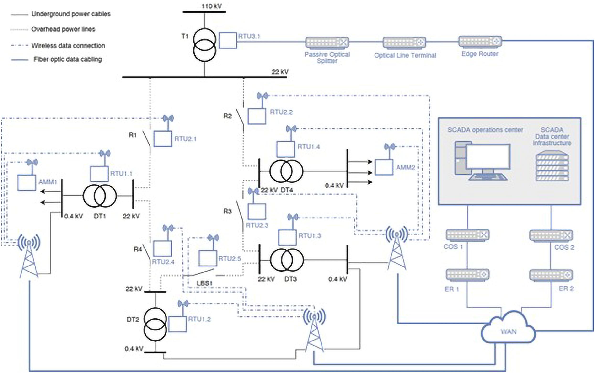
Visualization of an integrated power and communication network infrastructure within a smart grid framework, adapted from Ref.²⁴

Power grid

The power grid model consists of three distinct voltage levels and is structured around a primary substation featuring a 110/22 kV transformer as its main power source. The network is segmented into five separate overhead line sections (L1–L5), each integrated with a recloser (R1–R4) designed to disconnect fault currents when necessary. The final overhead line (L5) is further divided by a load break switch (LBS1), which typically remains open under standard operational conditions to maintain a radial network structure and minimize short-circuit currents.

If a fault arises, for example, in section L1, the system operator can use the LBS to reconfigure power delivery, allowing supply to be restored from an alternate direction. This process relies on remote control functionality enabled by a remote terminal unit (RTU), specifically RTU2.5, as indicated in Figure 1. RTU2.5 plays a vital role in maintaining network functionality. If a communication disruption or RTU2.5 failure occurs, immediate power restoration is hindered, leading to prolonged outages and negatively impacting system reliability indices such as the system average interruption duration index (SAIDI) and the system average interruption frequency index (SAIFI).

Additionally, the network incorporates four distribution transformers (DTs), which step down voltage levels to meet end-user demand through underground low-voltage (LV) cables (C1–C3). These cables are connected to the LV busbar, ensuring power distribution to different consumer categories. The interaction between the power grid and the communication network is crucial for maintaining operational efficiency. Compared to other components, the underground cable C4 is maintained exclusively through CM, as PM is not applicable.

Communication network

The communication network structure illustrated in Figure 1 consists of multiple RTU client devices, categorized by their connection method. The first category utilizes fiber optics to ensure reliable data transmission. Devices in this group communicate through a passive optical splitter (POS), an optical line terminal (OLT), and an edge router (ER). These routers serve as the interface to a wide area network (WAN), which may either be a private corporate network or a publicly accessible internet connection. When utilizing a public network, communication is secured through an encrypted virtual private network (VPN) tunnel to prevent unauthorized access.²⁴

In contrast to power grid components, which are subject to both preventive and CM, the elements of the communication network operate solely under a CM framework. Since preventive interventions are not feasible for these components, maintenance is conducted only in response to faults or failures. This distinction highlights the unique operational constraints and reliability strategies employed within the interconnected infrastructure.

Mathematical models for quantifying unavailability and cost

It is evident that the infrastructure architecture is very complex. The components that fall under both CM and PM and are described within the Introduction section are mutually interconnected in both networks. To solve the main goal of the paper, that is, the above-mentioned maintenance optimization problem when time dependent unavailability must be under control, it is necessary to develop three basic computing tools: first, a mathematical model representing all the infrastructure, second, a mathematical model for unavailability exploration of its components and third, a cost model to compute the cost of any system configuration. The system structure can be represented in different ways, for example, by means of a fault tree, a success tree, a Petri net, a neural network, binary decision diagrams, etc. Resulting from the author's previous experience,²⁵ the complex infrastructure can be optimally represented by the directed AG. Component unavailability, including both CM and PM, can be evaluated using the classic renewal theory,²⁰ which had to be adapted in this paper to express a special PM strategy applied to network components based on the deterministic time TP (time to start PM). Another innovation of the paper is the developed cost model, which estimates the cost of any network configuration, including components with the special PM strategy.

Directed AG

The directed AG is frequently used to describe relations or dependencies between all system components or subsystems. Figure 2 shows an example of a real-world system represented by AG, which describes the power grid part of the representative infrastructure shown in Figure 1. Formulation of the cost optimization problem section and Unavailability and cost of the optimal system configuration – results section will provide a detailed analysis and optimization of the power grid. The AG provides a structured approach for quantifying the unavailability of complex systems,²⁶ as it allows for a reflective description of a system's functionality.

Figure 2.

Directed AG representation of a power grid section, illustrating a distinct portion of the infrastructure.

The AG contains nodes and edges, with the S1 node being the sole exception, which describes the functionality of the entire power grid based on the performance of its subordinate subsystems and components that form internal and terminal nodes. Nodes are interconnected by edges, and the AG is acyclic, indicating that feedback loops are not permissible. Terminal nodes, such as DT2 or L2, are represented by blue squares and signify system components. The lifetime X, along with the repair time or time required for PM of a system component, is characterized by an appropriate probability distribution. Utilizing these distributions, the unavailability time progression of each component can be computed using the advanced renewal theory.²³

Subsystems of the power grid are internal nodes represented by blue triangles, such as u2 or u4. Components and subsystems (terminal and internal nodes) can be functioning correctly or in recovery time due to CM after a failure, or in scheduled shutdown (in recovery time due to PM). A node is functioning correctly if the count of functioning inferior nodes is greater than or equal to the number within the triangle. Otherwise, the node is not working, that is, it is either in failure (under CM) or in scheduled shutdown (under PM). For instance, the S1 node is functioning correctly if the number of functioning subordinate nodes is exactly 3. Similarly, the u1 node is functioning correctly if the number of functioning subordinate nodes is either 1 or 2.

As mentioned above, the exceptional node S1 describes the functionality of the entire power grid based on the functionality of its subordinate subsystems and components (both internal and terminal nodes). Therefore, from a computational perspective, it is necessary to find the unavailability function U(t) of the exceptional node S1. This function, which describes the time-dependent probability that a system is in a non-functioning state at time t due to either a failure or an ongoing maintenance, is a fundamental mathematical characteristic commonly employed to describe the reliability of complex systems. The unavailability function U(t) depends on the unavailability functions of both terminal and internal nodes. These functions, which can be computed using the unavailability models provided in the following subchapter act as inputs to obtain the unavailability function U(t) of the entire power grid.

Model for analyzing the unavailability of a terminal node with both CM and PM

To determine the unavailability function U(t) for the node S1, it is essential to develop a mathematical model and algorithm for quantifying the unavailability of terminal nodes that undergo both PM and CM.²⁷ Initially, the model with CM will be presented, and subsequently extended to incorporate the implementation of both PM and CM.

When applying CM, two interdependent random variables must be considered: the lifetime X, described by either the cumulative distribution function (cdf) F(t) or the probability density function (pdf) f(t), and the random time required to complete the repair, referred to as repair or recovery time Y, described by either the cdf G(t) or pdf g(t). Based on renewal theory and alternating renewal processes, the availability A(t) can be computed as follows,^28,29 equation (1):

A (t) = 1 - F (t) + \int_{0}^{t} h (x) [1 - F (t - x)] d x = R (t) + \int_{0}^{t} h (x) R (t - x) d x,

(1)where R(t) = 1 ‒ F(t) represents the reliability function, and h(x) denotes the renewal density of the corresponding alternating renewal process.

The unavailability U(t) is a complement of the availability in equation (1) to one, defined by equation (2):

U (t) = 1 - A (t) = F (t) - \int_{0}^{t} h (x) [1 - F (t - x)] d x

(2)

Equation (2) contains the renewal density h(x), which can be difficult to obtain in practice due to numerical complications. This is due to the fact that the renewal density is numerically represented as an infinite sum of probability densities,²⁸ each expressed as a convolution. Fortunately, equation (2) can be replaced by the equivalent equation (3), which is introduced by the following theorem, known as the Recurrent Linear Integral Equation, first mentioned and proved in Briš and Byczanski.²³

Theorem:

The unavailability U(t) in equation (2) is equivalent to the unavailability U(t) in the following equation (3).

U (t) = \int_{0}^{t} f (x) \cdot [1 - G (t - x)] d x + \int_{0}^{t} (f * g) (x) \cdot U (t - x) d x

(3)where * denotes convolution.

Subsequently, we consider PM strategies to sustain the operating status of the node. These pre-failure operations are typically less complex than CM activities required in the event of a failure. Clearly, each PM activity initiated at time TP, which serves as a decision variable in our maintenance optimization problem, necessitates some recovery time. The new random variable Z characterizes the recuperation time needed for carrying out any PM action starting at time TP, which is considered to be a deterministic characteristic of each component with PM. A component is in functioning state either up to the end of lifetime X, which is followed by restoration time Y due to CM or up to time TP, followed by recuperation time Z due to PM, whichever occurs first. In the course of both Y and Z, the component is in a non-functioning state. So PM actions can be regarded as low-cost interruptions that are usually much shorter than CM restoration times. For instance, PM can involve the procurement of a sufficient quantity of spare parts or regular training courses for company employees.

Special PM actions should be optimally implemented and carried out as close as possible before a failure occurs. Specifically, our model is particularly valuable for systems with high shutdown costs. To optimize the PM strategy (finding the optimal PM timing), total maintenance costs should be minimized while maintaining a decreasing trend in unavailability.

Equation (3) can be used to calculate the unavailability function U(t), but it must be modified respecting the new PM strategy comprising the deterministic time TP: the variable X is replaced with the variable V = min(X, TP), which constitutes the break of the functioning state. The random variable V, described by the distribution function F_V(t), can be derived using the elementary probability theory (probability of the union of two events), in equation (4):

\begin{aligned} F_{V} (t) & = P (V < t) = P (X < t) + P (T P < t) - P (X < t) . P (T P < t) \\ = 1 – P (V \geq t) = 1 – P (X \geq t) . P (T P \geq t) \end{aligned}

(4)

Therefore, the subsequent relations are valid, equation (5):

F_{V} (t) = F (t) f o r t < T P, F_{V} (t) = 1 f o r t \geq T P .

(5)

It means that equation (3) can be adapted in the following way:

For t < TP, we can use it in unchanged form, equation (6):

U (t) = U_{0} (t) = \int_{0}^{t} f (x) \cdot [1 - G (t - x)] d x + \int_{0}^{t} (f * g) (x) \cdot U (t - x) d x

(6)

And for t ≥ TP, we just apply the total probability theorem in the following equation (7):

\begin{aligned} U (t) = P (X < T P) ._{[\int_{0}^{T P} f (x) \cdot [1 - G (t - x)] d x + \int_{0}^{t} (f * g) (x) \cdot U (t - x) d x]} \\ + P (X \geq T P) \cdot [(1 - W (t - T P)) + \int_{0}^{t - T P} w (x) \cdot U (t - T P - x) d x] \end{aligned}

(7)where the first term in square brackets in equation (7) mathematically represents the component unavailability due to the recovery time Y needed for CM, and the second term represents unavailability due to the recuperation time Z needed for PM. The functions W(t) and w(t) are the distribution function and the pdf of the recuperation time Z, respectively.

The random variable V has the expectation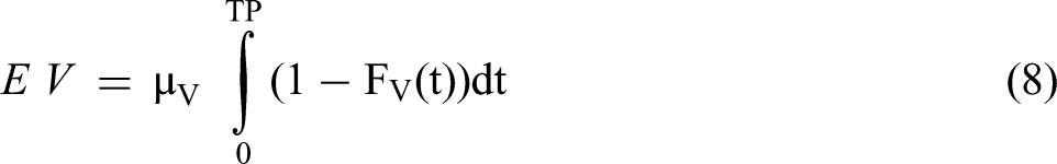 $μ_{V}$ that can be easily derived as follows, equation (8):

E V = μ_{V} \int_{0}^{TP} (1 - F_{V} (t)) dt

(8)

The effectiveness of this method for quantifying the unavailability of complex, multi-component, and highly reliable systems was successfully demonstrated in comparative studies in Briš and Byczanski²³ and Briš and Tran.²⁷

Cost model of the system configuration

The cost model for the system configuration can be derived by aggregating all contributions resulting from both CM and PM replacement interventions across all system components. Each component can function in various maintenance modes, with the cost of a single maintenance mode comprising two primary contributions: one from CM and the other from PM. The cost associated with CM is influenced by the mean number of recovery times due to both CM and PM during the mission time TM and CM parameters. Conversely, the cost of PM is determined by the decision variable TP and PM parameters. In practical scenarios, cost contributions are extracted from an annual database to calculate the average yearly cost for system configurations over a monitored period. Throughout this paper, the cost will be expressed in non-identified cost units based on the summation principle.

To determine the cost of a single system configuration, we simply sum up the costs of all maintenance modes of all system components. The cost of one maintenance mode of the j-th component $C_{T_{M}} (j)$ can be computed as follows, equation (9):

C_{T_{M}} (j) = n_{R} (j) . F (TPj) . C_{R} (j) + n_{R} (j) . R (TPj) . C_{PM} (j)

(9)where:

$n_{R} (j) = \frac{T_{M}}{MTTI (j) + MRT (j)}$ is the mean number of recovery operations of the j-th component per mission T_M,

MTTI(j) = E V = μ_V is the mean time to an intervention due to either CM or PM, MRT(j) is the mean recovery time of the j-th component due to either PM or CM, as given in equation (10):

MRT (j) = F (TPj) . MTRCM (j) + R (TPj) . MTRPM (j)

(10)where:

$MTRCM (j)$ is the mean recovery time due to CM,

$MTRPM (j)$ is the mean recovery time due to PM,

TPj is the decision variable of the j-th component defining the PM strategy,

$C_{R} (j)$ is the CM cost, that is, the cost of one CM action of the j-th component in cost units,

$C_{PM} (j)$ is the PM cost, that is, the cost of one PM action of the j-th component in cost units.

If the costs of all k system components given by equation (9) are added up, we obtain the total cost of one system configuration C_S, described by the following equation (11):

C_{S} = \sum_{j = 1}^{k} C_{T_{M}} (j)

\left(11\right)

For better understanding, the cost model can be enlarged and innovated in the case of the Weibull distribution, which is considered and justified in this paper, as indicated in Table 2. We see in equation (9) that the cost of each component is a complex function of TP, as well as μ_V. If the lifetime X follows the Weibull distribution (data of the power grid in Table 2), we can easily compute the mean time to an intervention due to either CM or PM, μ_V, as shown in equation (12):

E V = μ_{V} \int_{0}^{TP} (1 - F_{V} (t)) dt = \int_{0}^{TP} R_{V} (t) dt = \int_{0}^{TP} e^{- {(\frac{t}{θ})}^{2}} dt = θ \sqrt{π} \int_{0}^{\frac{\sqrt{2}}{θ} TP} \frac{1}{\sqrt{2 π}} e^{- {\frac{t}{2}}^{2}} dt = θ \sqrt{π} [ϕ (\frac{\sqrt{2}}{θ} TP) - \frac{1}{2}]

(12)

Table 2.

Characteristic values of the power grid components including reliability characteristics. The column TP_j,m (h) introduces the novel optimal values for the time to start PM.

Component	MTBF (h)	MTTRes (h)	β (–)	TP_j,m (h)^a	$C_{PM} (j)$	$C_{R} (j)$
Transformer T1 (110/22 kV)	26,310.71	4.403	2	25,180	45,000	115,000
Distribution transformer DT2 (22/0.4 kV)	43,800.36	0.361	2	41,600	21,000	54,000
Load break switch LBS1 (22 kV)	224,621.1	5.702	2	277,000	6000	12,000
Overhead line L1 (22 kV)	54,750.00	11.417	2	53,400	2000	5000
Overhead line L2 (22 kV)	41,714.29	11.417	2	40,700	2000	5000
Overhead line L3 (22 kV)	62,571.43	11.417	2	61,100	2000	5000
Overhead line L4 (22 kV)	48,666.67	11.417	2	47,500	2000	5000
Overhead line L5 (22 kV)	43,800.00	11.417	2	42,760	2000	5000
Underground cable C4 (0.4 kV)	153,967.54	85.000	2	–	–	11,000

The column TP_j,m (h) introduces the novel optimal values for the time to start PM.

In this case, E V = μ_V is also a function of TP: μ_V = μ_V(TP). Thus, we can conclude that the maintenance cost is a complex function of TP (time to start PM). Each component can be characterized by the maintenance cost dependency on TP. Unsurprisingly, the corresponding curve has its minimum.

Example: Consider two most important components of the power grid, DT2 and the transformer T1. By applying equation (9), the dependency of maintenance cost on TP is illustrated in Figure 3. Thus, the optimal PM initiation times can be identified as 41,600 h for DT2 and 25,180 h for T1, corresponding to the points of minimal maintenance cost. In both cases, the optimal time occurs slightly before the respective mean lifetimes—43,800 h for DT2 and 26,311 h for T1 (see Table 2).

Figure 3.

Relationship between the time to start PM (x-axis) and maintenance cost (y-axis) for components: (a) DT2 and (b) T1.

This TP ensuring minimal maintenance cost (denoted as TP_m) can be found for each component (the column TP_j,m in Table 2) of the power grid, resulting in an optimal system configuration with minimal maintenance cost. Most likely, the optimal system configuration keeps the time-dependent system unavailability during the mission time in acceptable limits because decreasing the TP results in a decrease of the mean time to intervention E V = μ_V, equation (12), due to either CM or PM, both causing interruptions in the operation time, that is, increasing the unavailability. Additionally, performing PM long before the mean lifetime MTBF would be very inefficient because the increase in the cost would be enormous.

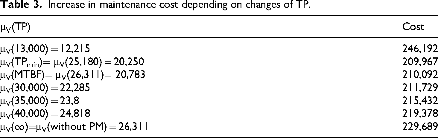
Increasing the TP causes increasing maintenance cost, whereas unavailability improves only moderately because μ_V(TP) is for TP > TP_min close to μ_V(MTBF), i.e. slightly above it. Although increasing the TP results in a moderate increase in μ_V (resulting in moderate unavailability improvement), the increase in the cost is significantly higher due to more expensive CM costs because CM becomes predominant for TP > MTBF compared to PM. For example, for the highly important component T1 (transformer) of the power grid, the following increase in the maintenance cost depending on the changes of TP is observed (Table 3).

Table 3.

Increase in maintenance cost depending on changes of TP.

$μ_{V} (TP)$	Cost
μ_V(13,000) = 12,215	246,192
μ_V(TP_min)= μ_V(25,180) = 20,250	209,967
μ_V(MTBF)= μ_V(26,311)= 20,783	210,092
μ_V(30,000) = 22,285	211,729
μ_V(35,000) = 23,8	215,432
μ_V(40,000) = 24,818	219,378
μ_V(∞)=μ_V(without PM) = 26,311	229,689

Formulation of the cost optimization problem

The optimization challenge addressed in this paper can be expressed as the following cost optimization problem:

It is necessary to find an optimal vector of the decision variables x = (x₁,…, x_k) that minimizes the objective function, defined here as the total maintenance cost C_S(x), as shown in equation (13):

m i n C_{S} (x)

(13)where:

C_S(x) is the objective function defined as the total cost of maintenance of a system configuration,

x = (x₁,…, x_k) ∈ R^k is the decision variable vector,

k is the number of system components, each with the decision variable TP_i (the time to initiate PM for the i-th component), which is optimized in this paper.

In most cases, C_S(x) is a complex linear or non-linear function of the decision variable vector

x = (x_{1}, \dots, x_{k}) = (T P_{1}, \dots, T P_{k})

representing parameters for which optimal values must be found. The cost of j-th component (for one maintenance mode)

C_{T_{M}} (j)

is characterized by equation (9), which is a complex function of the decision variable TP_j, having the minimal value TP_j,m, as demonstrated in Figure 3. Thus, the optimization problem can be easily solved by finding the values TP_j,m of all components that minimize the objective function (15). The found decision variable vector (TP_1,m,…, TP_k,m) can be subsequently used to define the optimal system configuration, the unavailability of which will be analyzed in Unavailability and cost of the optimal system configuration – results section. Note also that due to the obvious convexity of the cost functions, Figure 3, with minima in feasible values, Table 2, the minimization problem can be formulated as an unconstrained one.

In some cases, it is necessary to solve a multi-objective optimization problem, or additional complex constraints are added (e.g., restrictions on system operation). In such cases, a global optimum must be found that does not violate any constraints. Therefore, all tasks connected with the given optimization problem (optimization, objective functions, and constraints) must be handled concurrently, each depending on the others. Solving such problems requires advanced numerical algorithms.^30–32

In the earlier research work, such as Briš and Tran,³³ the optimization problem with restrictions was solved. Another tool to solve similar optimization problems is genetic algorithms (GA), which have been widely used in prior research. For instance, Munoz³⁴ employed GA to optimize surveillance testing and maintenance. Among others, Cacereño³⁵ and Topolanek et al.³⁶ also applied GA in their studies.

Unavailability and cost of the optimal system configuration – results

Although the representative infrastructure consists of two separate parts (power grid and communication network), the PM optimization was performed only on the power grid because PM of the communication network components is not allowed. The basic input data for both unavailability and cost computation of the power grid are provided in Table 2, which contains the reliability characteristics of all input components (terminal nodes) as well as the maintenance cost of both CM and PM. The input data are adopted from Vrtal et al.,²⁴ where the time to failure of all power grid components follows the Weibull distribution with the shape parameter β = 2, as ageing of power grid components is linear.^24,25

The distribution function of the time to failure X can be expressed using the parameters MTBF and β included in Table 2 as follows:

F (t) = 1 - e^{- [\frac{t}{M T B F} \cdot Γ (1 + \frac{1}{β})]}

where

Γ (1 + \frac{1}{β})

is the gamma function, which can be defined via a convergent improper integral for positive real numbers z:

Γ (z) = \int_{0}^{\infty} t^{z - 1} e^{- t} d t

In the field of electrical engineering, the recovery time Y is predominantly characterized by an exponential distribution, based on MTTRes specifications derived from authentic data.²⁵ The distribution function of the random variable Y (random recovery time) can be expressed using the parameter MTTRes included in Table 2 as follows:

G (t) = 1 - e^{\frac{t}{MTTRes}}

The underground cable C4 is a highly reliable component for which PM is impossible. Prompt PM in this analysis is assumed because the recovery time Z due to PM was very small compared to the recovery time due to CM. Therefore, it can be neglected. Table 4 contains the reliability characteristics of the remaining communication and control components from Figure 1. Table 4 is adopted according to Briš et al.²⁵ and Vrtal et al.²⁴ (electricity network) and the Optical switch by Braun teleCom³⁷ (communication network).

Table 4.

Characteristic values of the communication and control components.

Component	MTBF (h)	MTTRes (h)	β (–)
Edge Router ER1	16,246.780	0.780	2
Edge Router ER2	16,246.780	0.780	2
Core Optical Switch COS1	5,000,014.000	14.000	2
Core Optical Switch COS2	5,000,014.000	14.000	2
Aerial Optic fiber AO4	500,000.000	6.000	2
Aerial Optic fiber AO5	1093,750.000	6.000	2
Aerial Optic fiber AO6	500,000.000	6.000	2
Aerial Optic fiber AO7	1093,750.000	6.000	2
Buried Optic fiber BO1	821,875.000	12.000	2
Buried Optic fiber BO3	1753,333.333	12.000	2
Buried Optic fiber BO4	1753,333.333	12.000	2
Remote Terminal Unit RTU	100,048.000	48.000	2
SCADA operation and data center	175,200.000	184.600	2
Base Transceiver Station BTS	100,000.000	4.000	2
Wide Area Network WAN	100,000.000	4.000	2

Optical communication components are very reliable. For example, the Bran TeleCom OSW-2 switch has an MTBF equal to or greater than 106 h.

If the probability distributions of the random variables X and Y are now fully determined for each component, the functions F(t), f(t), G(t), and g(t) are known, and integral equations (6)‒(7) can be solved to obtain time dependent unavailability evolutions. These evolutions act as inputs to AG that are needed to obtain the unavailability function U(t) of the entire infrastructure.

The unavailability evolution U(t) of the entire network, denoted by the SS node of the AG in Figure 4, over the mission time T_M = 6 years is demonstrated in Figure 5 as the SS-curve. This function, U(t), provides an insight into the time-dependent likelihood that the network might experience a failure at time t due to a malfunction or an ongoing repair process. The same Figure 5 shows the unavailability evolution (S1-curve) of the power grid S1 (subnetwork in Figure 1) represented by the AG in Figure 2, before the implementation of PM. It is evident that the unavailability function in both cases is sharply increasing in the course of the entire mission time T_M. The maximum unavailability value by the end of the mission time T_M = 6 years is 1.343e-3 for the entire network and 4.622e-4 for the power grid S1 without PM. Implementation of PM, which is possible only for the power grid part of the infrastructure, has the potential for improving the unavailability of both evolutions. If all components of the power grid undergo further PM (except for the underground cable C4 where PM is impossible), the unavailability evolution over the mission time T_M = 6 years of the optimal system configuration, found according to Formulation of the cost optimization problem section, brings the continuous line in Figure 6. For comparison purposes, Figure 6 also demonstrates the unavailability evolution of the configuration without PM, see the dashed line. Both evolutions coincide until the starting time of PM, with the PM starting time here being of the transformer T1.

Figure 4.

AG of the representative interconnected infrastructure from Figure 1.

Figure 5.

Unavailability evolution of the representative interconnected infrastructure SS from Figure 1 in comparison with the unavailability of the power grid S1, within the mission time of 6 years and without PM.

Figure 6.

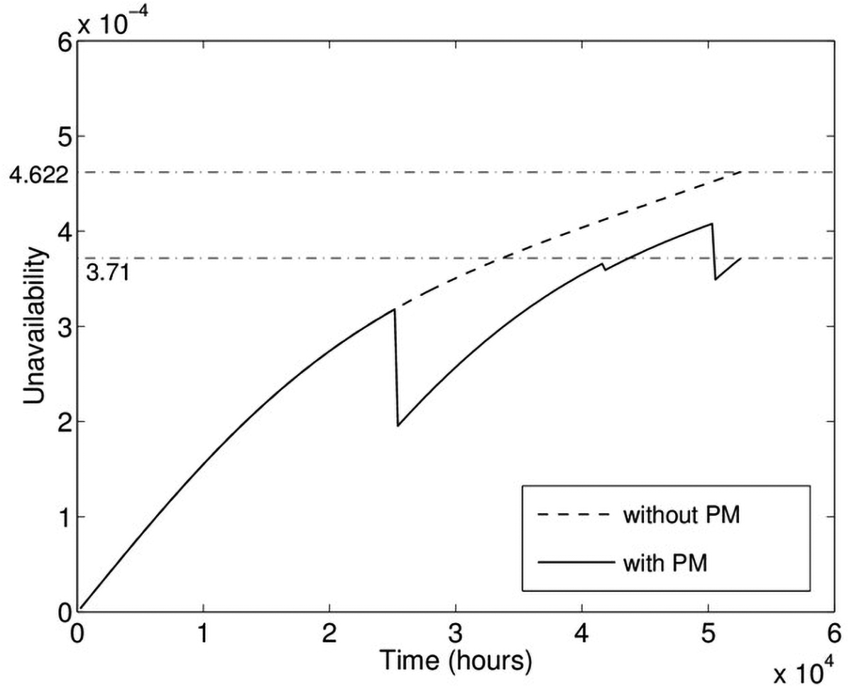
Unavailability evolution of the power grid with optimal PM and without PM, within the mission time of 6 years.

In the optimal configuration, two characteristic drops in the system unavailability resulting from PM of the transformer T1 (at times 25,180 and 50,360 h), as well as one mild decrease in the unavailability caused by PM of DT2 (at time 41,600 h) can be seen. This result is not surprising because both components are minimal cuts of the 1^st order (failures of both components result in the failure of the entire power grid). PM of other components influences the unavailability evolution insignificantly due to the fact that either they are highly reliable (C4 has MTBF almost six times longer) or the components are included in minimal cuts of the second order, which means that a failure of network can be caused solely by simultaneous malfunction of at least two components. Both situations are rare events, and for this reason, the unavailability is influenced negligibly.

The total maintenance cost of the optimal configuration decreased significantly—by approximately 8.53%—from 323,986 to 296,357 cost units. In comparison, the configuration without PM incurs a cost of 323,986.

Future research can introduce maintenance modeling and optimization of complex systems, such as ships and ports, which include electrical and thermal systems. Subsequent advanced sensitivity analyses and machine learning to balance reliability and savings³⁸ can attract users through interactive applications.³⁹

Conclusions

The maintenance optimization problem formulated in Formulation of the cost optimization problem section was successfully solved for the selected representative infrastructure. The primary decision variable in the optimization problem is the time to initiate PM (TP). To address this optimization challenge, previously developed methods for unavailability quantification based on renewal theory were enhanced. The method for unavailability exploration was newly modified to include mathematical models for calculating the system components operating in different maintenance modes. Renewal theory is innovated here to implement a special PM strategy, optimally pursued just before a failure is expected to occur. A component operates either up to the failure time X (lifetime) followed by the restoration time due to CM or up to the time TP, followed by the recuperation time Z due to PM, whichever occurs first. This means that PM actions are planned as low-cost interruptions, which are typically shorter than CM restoration times.

To estimate the cost of various system maintenance configurations, a convenient cost model was created. Initially, optimal values of decision variables TPs minimizing the component's cost of the optimized power grid were found and subsequently used to configure the optimal system configuration. The dependence of unavailability on time was computed for a given mission time and compared with the configuration without PM. The results show that both the system unavailability and the total maintenance cost of the optimal system configuration significantly decreased. The power grid unavailability decreased at the end of the mission to a value of 3.71e-4 (about 20%), and the total maintenance cost decreased to 296,357 cost units (about 8.53%). The results highlight that complementing scheduled visits triggering PM replacements leads to a reduction in the total maintenance cost.

Most of cost-unavailability maintenance optimization algorithms are based on constant unavailability values, such as in Cacereño et al.³⁵ The novel methodology for computing the unavailability course of a complex system and its components is particularly applicable to systems that are not yet stabilized in an asymptotic unavailability mode. It is particularly relevant when short-term unavailability changes, and time evolutions can play a critical role—for example, in safety-related applications. A typical example of such a system is the emergency core cooling system used in nuclear power plants.³²

From the computational perspective, the process of unavailability exploration of the selected infrastructure is numerically intensive and time-consuming. Despite the complexity, the time required for the demonstrated calculations did not exceed 1 h. All calculations, including both the unavailability and cost computing algorithms for different system configurations represented by AG, were numerically implemented using the advanced programming MATLAB language. These computations were performed on a system equipment with the following specifications: Intel (R) Core™ i7-3770 CPU @ 3.9 GHz, 8.00 GB RAM.

Footnotes

Abbreviations

ORCID iDs

Radim Briš

Pavel Praks

Matěj Vrtal

Dejan Brkić

Author contributions

Radim Briš contributed to writing–review and editing, writing–original draft, visualization, validation, investigation, software, methodology, formal analysis, conceptualization, and funding acquisition. Pavel Praks contributed to writing–review and editing, validation, investigation, data curation, methodology, formal analysis, conceptualization, funding acquisition, and project administration. Radek Fujdiak contributed to writing–review and editing, supervision, validation, investigation, data curation, methodology, formal analysis, conceptualization, funding acquisition, and project administration. Matěj Vrtal contributed to writing–review and editing, validation, investigation, data curation, methodology, and formal analysis. Dejan Brkić contributed to writing–review and editing, conceptualization, and funding acquisition.

Funding

The authors disclosed receipt of the following financial support for the research, authorship, and/or publication of this article: This work was supported by the Operational Programme Johannes Amos Comenius, the Ministry of the Interior of the Czech Republic in the “Open call in security research 2023–2029” grant programme, Ministry of Science, Technological Development and Innovation of the Republic of Serbia, VSB-Technical University of Ostrava, Czech Republic (grant number: CZ.02.01.01/00/23_021/0008759, VK01030109, 451-03-136/2025-03/200102, SGS 2 KAM 2024, No. SP2024/017).

Declaration of conflicting interests

The authors declared no potential conflicts of interest with respect to the research, authorship, and/or publication of this article.

Appendix

Notations

References

Ding

S-H

Kamaruddin

. Maintenance policy optimization—literature review and directions. Int J Adv Manuf Technol 2015; 76: 1263–1283.

Lee

Lapira

Bagheri

, et al. Recent advances and trends in predictive manufacturing systems in big data environment. Manuf Lett 2013; 1: 38–41.

Badia

Berrade

. Optimum maintenance policy of a periodically inspected system under imperfect repair. Adv Operat Res 2009; 2009: 1–13, Article ID 691203.

Ben Mabrouk

Chelbi

Aguir

, et al. Optimal maintenance policy for equipment submitted to multi-period leasing as a circular business model. Sustainability 2024; 16: 5238.

Tamura

. Structure of an optimal maintenance policy for a semi-Markovian deteriorating system with major and minor failures. Qual Reliab Eng Int 2022; 38: 3002–3016.

Liu

Chen

Jin

, et al. Optimum opportunistic maintenance schedule incorporating delay time theory with imperfect maintenance. Reliab Eng Syst Saf 2021; 213: 107668.

Bai

Wang

, et al. Optimization algorithm of association rule mining for heavy-haul railway freight train fault data based on distributed parallel computing. Sci Prog 2024; 107: 1–18.

Kıvanç

Fecarotti

Raassens

, et al. Condition-based maintenance for multi-component systems: a scalable optimization model with two thresholds. Reliability Eng Syst Safety 2025; 254: 110634.

Zhang

Qian

Dui

, et al. Opportunistic maintenance strategy of a heave compensation system for expected performance degradation. Mainten Reliab 2021; 23: 512–521.

10.

Luo

Liu

Wang

, et al. Tolerance analysis for automobile transmission shaft based on minimum cost and reliability target. Sci Prog 2020; 103: 1–15.

11.

Zhang

Coit

. Deep reinforcement learning for dynamic opportunistic maintenance of multi-component systems with load sharing. IEEE Trans Reliab 2022; 72: 863–877.

12.

Wang

Cui

, et al.

A predictive opportunistic maintenance policy for a serial–parallel multi-station manufacturing system with heterogeneous components.

Reliab Eng Syst Saf 2025; 256: 110711.

13.

Németh

Kocsis

Takács

, et al. Maintenance schedule optimisation for manufacturing systems. IFAC-PapersOnLine 2020; 53: 319–324.

14.

Zhang

, et al. Development of a preventive maintenance strategy for an automatic production line based on group maintenance method. Appl Sci 2018; 8: 1781.

15.

Manzini

Regattieri

Pham

, et al. Maintenance for industrial systems (Vol. 1). London: Springer, 2010.

16.

de Jonge

Klingenberg

Teunter

, et al. Optimum maintenance strategy under uncertainty in the lifetime distribution. Reliab Eng Syst Saf 2015; 133: 59–67.

17.

Zio

Compare

. Evaluating maintenance policies by quantitative modeling and analysis. Reliab Eng Syst Saf 2013; 109: 53–65.

18.

Wang

Limmer

Van Nguyen

, et al. Optimizing the maintenance schedule for a vehicle fleet: a simulation-based case study. Eng Optim 2021; 54: 1258–1271.

19.

Tang

. Reliability assessment for systems suffering competing degradation and random shocks under fuzzy environment. Sci Prog 2020; 103: 1–23.

20.

Cox

. Renewal theory. London: Methuen Young Books, 1962.

21.

Scarf Philip

. On the application of mathematical models in maintenance. Eur J Oper Res 1997; 99: 493–506.

22.

Jardine

Tsang

. Maintenance, replacement, and reliability: theory and applications. CRC Press, 2005.

23.

Briš

Byczanski

. On innovative stochastic renewal process models for exact unavailability quantification of highly reliable systems. Proc Inst Mech Eng Part O: J Risk Reliabil 2017; 231: 617–627.

24.

Vrtal

Fujdiak

Benedikt

, et al. Time-dependent unavailability exploration of interconnected urban power grid and communication network. Algorithms 2023; 16: 561.

25.

Briš

Byczanski

Goňo

, et al. Discrete maintenance optimization of complex multi-component systems. Reliab Eng Syst Saf 2017; 168: 80–89.

26.

Briš

. Parallel simulation algorithm for maintenance optimization based on directed acyclic graph. Reliab Eng Syst Saf 2008; 93: 874–884.

27.

Briš

Tran

. Newly enhanced computing algorithm to quantify unavailability of maintained multi-component systems. In: Haugen A, Barros A, van Gulijk C, et al. (eds) Safety and reliability–safe societies in a changing world. London: CRC Press, 2018, pp. 931–936. DOI: 10.1201/9781351174664-117.

28.

Ross

. Applied probability models with optimization applications. New York: Dover Publications, Inc., 1992.

29.

Nakagawa

. Maintenance theory of reliability. London: Springer-Verlag, 2005.

30.

Fletcher

. Practical methods of optimization. John Wiley & Sons, 2000.

31.

Vaurio

. Optimization of test and maintenance intervals based on risk and cost. Reliab Eng Syst Saf 1995; 49: 23–36.

32.

Harunuzzaman

Aldemir

. Optimization of standby safety system maintenance schedules in nuclear power plants. Nucl Technol 1996; 113: 354–367.

33.

Briš

Tran

NTT

. Optimization of maintenance policies for complex and highly reliable multi-unit systems. In: Čepin

Briš

(eds) Safety and reliability – theory and applications. London: Taylor & Francis Group, 2017, pp. 403–411.

34.

Munoz

Martorell

Serradell

. Genetic algorithms in optimizing surveillance and maintenance of components. Reliab Eng Syst Saf 1997; 57: 107–120.

35.

Cacereño

Greiner

Galván

. Multi-objective optimum design and maintenance of safety systems: an in-depth comparison study including encoding and scheduling aspects with NSGA-II. Mathematics 2021; 9: 1751.

36.

Topolanek

Krcal

Foltyn

, et al. Optimization method for short circuit current reduction in extensive meshed LV network. Int J Electr Power Energy Syst 2023; 152: 109203.

37.

Optical Switch. Braun teleCom GmbH, Hanover, Germany (Version 2.0). Available at: https://shop.brauntelecom.de/out/media/Optical-switch.pdf (accessed 20 February 2025).

38.

Praks

Rasmussen

Lye

, et al. Sensitivity analysis of parameters for carbon sequestration: symbolic regression models based on open porous media reservoir simulators predictions. Heliyon 2024; 10: e40044.

39.

Brkić

Praks

Buchlovská Nagyová

, et al. Software tool with implemented optimisation algorithms for sophisticated control system (SCS) of selected waste-to-energy processes. Software. Ostrava, Czech Republic: VSB - Technical University of Ostrava.

Maintenance optimization for unavailability enhancement of representative interconnected infrastructure based on minimum cost

Abstract

Keywords

Introduction

Background

Literature review

Overview

Representative infrastructure

Power grid

Communication network

Mathematical models for quantifying unavailability and cost

Directed AG

Model for analyzing the unavailability of a terminal node with both CM and PM

Cost model of the system configuration

Formulation of the cost optimization problem

Unavailability and cost of the optimal system configuration – results

Conclusions

Footnotes

Abbreviations

ORCID iDs

Author contributions

Funding

Declaration of conflicting interests

Appendix

References