Multiobjective optimization for the bed structure of a CNC gantry machine tool based on neural networks and intelligent optimization algorithms

Abstract

This study proposes a multiobjective optimization design method for the bed structure of CNC gantry machine tools to enhance their mechanical performance. A sensitivity analysis was first conducted to identify the key dimensions affecting the bed's mass and static and dynamic characteristics, which were then selected as optimization variables. Design of experiments was employed to obtain target values under various design variables, and the response surface method combined with neural network algorithms was utilized to approximate and validate the objective functions. Subsequently, the entropy weight method was applied to calculate the weight coefficients of multiple optimization objectives, establishing a comprehensive performance optimization model for the bed structure. Using MATLAB, three intelligent algorithms—simulated annealing, genetic algorithm, and particle swarm optimization—were employed to solve the optimization model. Comparative results before and after optimization demonstrated that the optimized bed structure achieved a maximum deformation reduction of 9.41%, a 5.75% increase in the first-order natural frequency, a 1.23% reduction in maximum stress, and a 0.64% decrease in mass. The proposed optimization method offers a novel approach for simultaneously reducing the weight of structural components while enhancing their static and dynamic performance.

Introduction

With the rapid development of CNC technology and continuous scientific advancements, CNC machine tools have been widely applied in the aerospace industry and mechanical processing sectors. High-speed gantry five-axis machining centers are primarily used for the high-speed, efficient, and high-precision processing of large complex molds and aluminum alloy structural parts, making them critical processing equipment in mechanical manufacturing. Therefore, improving the performance and precision of five-axis machining centers is one of the urgent tasks in current research and engineering fields. ¹ Meanwhile, with global resources and energy becoming increasingly scarce, reducing production costs has become an important topic in today's manufacturing industry. In the current economic environment, the machine tool industry focuses on enhancing performance while reducing costs, conserving energy, and minimizing environmental impact. ² By conducting structural optimization design of key components of five-axis machining centers, it is possible to enhance their static and dynamic performance and achieve lightweight design, thereby improving precision and controlling costs. Structural optimization design not only helps to enhance the overall performance of the machine tools but also effectively reduces the consumption of production resources, ultimately achieving the goal of efficient and low-cost machining.

Modern machine tool design involves numerous variables and constraints, and traditional single-objective optimization methods often need help to manage this complexity effectively. Multiobjective optimization can systematically consider these factors, thereby better-addressing design challenges. Wang et al. ³ review advances geometric accuracy design for CNC machine tools by integrating sustainable manufacturing into accuracy allocation frameworks. It proposes an enhanced Sobol-based global sensitivity analysis model that significantly improves computational efficiency, and pioneers a digital twin-enabled verification system. The study establishes a theoretical paradigm for multiobjective optimization that simultaneously addresses precision, cost-effectiveness, and carbon footprint reduction.

Guo et al. ⁴ conducted a sensitivity analysis on the geometric errors of five-axis machine tools and achieved optimal accuracy through multiobjective optimization, significantly enhancing machining precision. Ic et al. ⁵ propose a novel TOPSIS-FFNN integrated model that addresses the limitations of subjectivity inherent in the criterion weights of traditional multicriteria decision-making approaches for selecting machining centers. By utilizing a feedforward neural network to capture the complex nonlinear relationships among criteria, the model significantly enhances computational efficiency and robustness. Liu et al. ⁶ propose a topology optimization framework for the layout of stiffeners based on the ground structure method. By introducing a thickness penalization parameter (p = 3), the thickness of the stiffeners is explicitly parameterized to eliminate intermediate values. Verified through impact modal testing (with a finite element analysis error of <3.61%), this method enhances the first six natural frequencies of the spindle box of a horizontal machining center by 5.58% to 19.52%. Tong et al. ⁷ are the first to apply the particle swarm optimization (PSO) algorithm to the multiobjective optimization design of machine tool spindle-bearing systems, while considering bearing preload and position as design variables. The research focuses on the simultaneous optimization of conflicting objectives, including natural frequency, static stiffness, and friction torque. By constructing a Pareto front, the study provides a basis for design decision making, ultimately achieving an improvement in natural frequency of 6% to 11% and an enhancement in static stiffness of approximately 26%. Chan et al. ⁸ validated the static stiffness and dynamic characteristics of a three-axis machining center through finite element analysis and experimental verification. They significantly reduced the mass of critical components using topology optimization, enhancing both stiffness and natural frequency. Additionally, they integrated numerical techniques and predictive diagnostics to improve the precision of the rolling cam rotary table, demonstrating a hybrid diagnostic and numerical strategy similar to evaluations based on neural networks. Tian et al. ⁹ proposed a multiobjective optimization method based on the NSGA-II algorithm for process parameters. Although product multiobjective optimization is increasingly emphasized in green manufacturing, the approach needs a detailed discussion on balancing different objectives, resulting in a lack of systematization in the optimization process. Chan et al. ¹⁰ investigated the static and dynamic characteristics of a gantry-type high-precision machine tool using finite element analysis and topology optimization methods. They optimized to reduce the mass of components, thereby enhancing stiffness and natural frequency, with experimental and simulation errors of <1.56%. This significantly improved the machine tool's performance and energy efficiency. Ullah et al. ¹¹ conducted finite element analysis and experimental validation to study the dynamic and static characteristics of a CNC lathe. Through topology optimization, they reduced the mass of the machine base by 47.1 kg while increasing the first three natural frequencies by approximately 1.51%. The optimized static deformation was reduced by 10.2%, significantly enhancing the machine tool's stiffness and vibration resistance, covering topology optimization and structural dynamics under various working conditions. Shen et al. ¹² introduced a novel dynamic design optimization approach for the overall structure of machine tools. They employed an adaptive growth method for the internal rib layout of the machine tool structure and conducted optimization studies using dynamic sensitivity analysis. However, the validation of the optimization scheme was insufficient. Zhang et al. ¹³ utilized a combination of sensitivity analysis and central composite design to optimize the spindle structure of CNC gantry milling machines. The results showed a mass reduction of 3.11%, a total deformation reduction of 6.87%, and an increase in the first natural frequency by 2.56%. Chen et al. ¹⁴ optimized the design of the grinding wheel headstock, B-axis housing, and column using a backpropagation (BP) neural network and genetic algorithm (GA), achieving a 21% reduction in maximum deformation and increases of 6.36%, 9%, 6.4%, and 2.84% in the first four natural frequencies, respectively. Li et al. ¹⁵ optimized the beam structure of a computer numerical control milling machine using sensitivity theory and the NSGA-II algorithm; the optimization resulted in a 7.45% reduction in mass, a 3.08% reduction in deformation, and a 0.42% increase in modal frequency. Ji et al. ¹⁶ employed response surface methodology (RSM) to establish an approximate functional relationship between five decision variables and four performance indices. Subsequently, they formulated the optimization objective through principal component analysis by combining the four performance indices. A new hybrid algorithm integrating simulated annealing (SA) and PSO was developed to tackle structural optimization problems. The computational analysis revealed a linear relationship between the mass of moving parts and energy consumption, though the algorithm's convergence speed and potential local optima might be areas for improvement. Introducing more optimization techniques or refining algorithm parameters could enhance the stability and efficiency of optimization results. Ma et al. ¹⁷ proposed a multiobjective optimization design model for machine tools that comprehensively considers static and dynamic stiffness constraints. This was achieved through an improved reduced-order dynamic model, multipoint constraints, and a joint substructure stiffness model described by screw theory. The optimized machine tool's static and dynamic performance was significantly improved using neural network function approximation and genetic algorithm optimization. Stiffness tests and experimental modal analysis indicated that the errors between the optimized model and experimental results were below 8.24% and 15.61%, respectively. Hao et al. ¹⁸ leveraged the adaptive growth characteristics of leaf veins to utilize a variable cross-section ribbed plate structure, and combined it with a genetic algorithm to optimize a BP neural network for the establishment of a high-accuracy surrogate model. The marine predator algorithm was employed for multiobjective optimization. This approach significantly enhanced the performance of the column structure, resulting in a 32.89% increase in the first-order natural frequency and an average reduction of 2.5% in static deformation.

In summary, various studies have made significant explorations in the multiobjective optimization of machine tools, aiming for a comprehensive and reasonable enhancement of the mechanical performance of gantry machine tools. This article investigates a multiobjective optimization design method for the structure of CNC gantry machine tool beds. A multiobjective optimization design method was established specifically for the bed of a particular gantry machine tool. Static mechanical and modal analyses were performed on the gantry machining center bed, providing a reference for subsequent optimization design. Multiobjective optimization modeling of the bed was then carried out, and sensitivity analysis was used to identify parameter variables with significant impacts on the optimization objectives. Design of experiments (DOE) was conducted using central composite design (CCD), Box-Behnken design (BBD), and Latin hypercube sampling design (LHS) to obtain 189 samples for the neural network fitting of the objective functions. The entropy weight and CRITIC methods were employed to calculate weight coefficients for each optimization objective, establishing a comprehensive aim of the performance function. Finally, intelligent algorithms such as SA, GA, and PSO were applied using MATLAB software to solve the optimization problem. A comparative analysis of the results before and after optimization verified the effectiveness of the proposed multiobjective optimization design method for the machine tool bed. The research content flowchart of this study is shown in Figure 1.

Figure 1.

Research content flow chart.

Materials and methods

Bed optimization design method and process

The specific process of multiobjective optimization design for machine tool bed is as follows:

Add initial geometric parameters, material properties (HT300), and constraint conditions.

Using SolidWorks software for parametric modeling and generating parametric 3D model.

Perform finite element simulation analysis using ANSYS Workbench software, including two simulation analysis methods: static analysis and modal analysis. Among them, static analysis requires the application of fixed constraints on the bottom surface of the bed and a load consisting of 2242.5 kg of self-weight and cutting force, while modal simulation applies fixed constraints at the bed bottom.

Conduct sensitivity analysis based on formulas 1 and 2 to screen out the key dimensions W, R₁, R₂, and L₂ that affect the performance of the bed.

Adopting a mixed experimental design strategy for experimental design, 189 sample points were generated through CCD experimental design method, BBD experimental design method, and LHS experimental design method.

Weight calculation, using CRITIC entropy weighting method combined weighting based on formulas 8 and 9.

Multiobjective-optimization based on formula 20, the constraint model is solved using SA, GA, and PSO algorithms.

Return the optimal solution and verify: After verifying the performance improvement of the bed, output the optimized design parameters W, R₁, R₂, and L₂.

The material of the bed and the function of the machine tool

The multiobjective optimization design in this article is based on the QLM27100-5X bridge-type five-axis linkage gantry machining center, which is shown in Figure 2.

Figure 2.

Appearance and component diagram of bridge gantry machining center.

The main structure of a gantry machining center consists of critical mechanical components such as the bed, beam, ram, spindle box, and workbench. The spindle box features an adjustable angle design, allowing for flexible adjustment of the spindle's machining angle. This design facilitates the machining of the sides or internal cavities of workpieces.

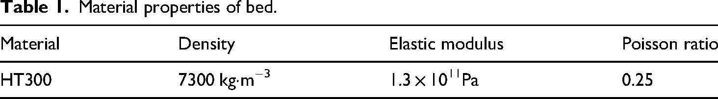
The machine bed, the supporting part of the machine, bears the weight of components such as the machine's beams, carriages, rams, and spindles and is, therefore, subjected to high loads. To ensure the machining accuracy of the machine tool, it is necessary to ensure that the column has a more remarkable ability to resist deformation under a large static and dynamic load, that is, a higher static stiffness and dynamic stiffness. The material used for the bed is HT300, and the material properties are shown in Table 1. The weight of the left and right parts mass 2242.5 kg. The geometric dimensions are: length 2500 mm, width 660 mm, and height 1255 mm. The arrangement of the inner rib plate is horizontal and vertical crossing, and the middle is hollowed.

Table 1.

Material properties of bed.

Material	Density	Elastic modulus	Poisson ratio
HT300	7300 kg·m−3	1.3 × 1011Pa	0.25

When performing the static analysis of the machine bed, the fixed constraints are applied to the two bottom surfaces of the machine bed, which bear the weight of components such as the machine tool beam, carriage, ram, and spindle, as well as the self-weight and cutting resistance.

Machine bed simulation analysis method

Solidworks software was used to model and parametrize the machine bed structure. ANSYS Workbench software provided an interface for connecting Solidworks to ANSYS Workbench. The machine bed's 3D model was imported into ANSYS Workbench for simulation analysis. The element type is set to: solid187. Due to the good consistency between the simulation results and the modal vibration experiment results, the mesh convergence is considered satisfactory. The boundary conditions for the static analysis are as follows: the bottom of the bed is set as a fixed constraint, bearing the weight of components such as the spindle, beam, its own weight, and cutting resistance. For the modal analysis, the boundary condition is that the bottom is fixed. The static constraint diagram of the bed is shown in the Figure 3.

Figure 3.

Static constraint diagram of the bed.

Finite element static analysis method of the machine bed

Structural static analysis is a fundamental and widely applied method used to determine the displacements, stresses, strains, and internal forces of a structure or component under loads without inertial and damping effects. During the operation of a CNC gantry machine, the bed is subjected to various forces, which can result in slight deformations and stress variations. Excessive deformation may lead to structural instability of the bed, while excessive stress could cause structural damage. Therefore, conducting a structural static analysis of the bed is essential to investigate its ability to resist deformation and failure under various forces. Structural static analysis provides a foundation for subsequent optimization design aimed at enhancing the static performance of the bed.

Finite element modal analysis method of the machine bed

Modal analysis is a method used to study the dynamic characteristics of mechanical structures. Modal analysis determines a structure or mechanical component's natural frequencies and mode shapes. Structural design typically uses this analysis to identify potential resonance issues and ensure the structure can endure vibrations without excessive deformation or stress. When the bed of a machine tool is subjected to external excitations, if the frequency of the induced vibrations matches or is close to one of the bed's natural frequencies, resonance can occur. ¹⁹ Resonance affects the machining precision and stability of the machine tool and can cause varying degrees of damage to the bed's structure. ²⁰ Therefore, performing a modal analysis on the bed is essential to ensure its stability during operation, understand its ability to resist disturbances, and use this information as a target for subsequent optimization.

The modal analysis process is similar to finite element static analysis. However, its results depend only on the bed's material properties and constraints without considering external loads.

Multiobjective optimization modeling of the machine bed

Sensitivity analysis methods

The bed structure comprises numerous dimensional parameters, each influencing the bed's performance to varying extents. Sensitivity analysis selects the factors significantly impacting the optimization objectives as design variables to simplify the optimization model and reduce computational workload. Sensitivity analysis primarily involves assessing the degree to which changes in design variables affect the target variables within experimental designs. Sensitivity analysis is widely used to investigate the influence of parameter variations on system characteristics in both linear and nonlinear systems.

Due to its diagnostic and predictive capabilities, sensitivity analysis is frequently used to evaluate the impact of inputs on outputs, playing a crucial role in fields such as energy systems and material performance research. ²¹ Depending on the level of computational precision, sensitivity analysis methods can be categorized into first-order, second-order, and higher-order sensitivity analyses. Mathematically, if the function F(x) is differentiable, its first-order sensitivity can be expressed as follows. ²²

$$S={\displaystyle \frac{\mathrm{\partial }F(x)}{\mathrm{\partial }{x}_j}\mathrm{or}S={\displaystyle \frac{\mathrm{\Delta }F(x)}{\mathrm{\Delta }{x}_j}}}$$

(1)

In addition to the first-order sensitivity, high-order sensitivity can be obtained, as shown below.

$$S={\displaystyle \frac{\mathrm{\partial }F\mathrm{″}(x)}{\mathrm{\partial }{x}_j\mathrm{″}}\mathrm{or}S={\displaystyle \frac{\mathrm{\Delta }F\mathrm{″}(x)}{\mathrm{\Delta }{x}_j\mathrm{″}}}}$$

(2)

In sensitivity analysis of variables concerning a specific objective, the larger the absolute value of a variable's sensitivity, the greater its impact on the objective. A positive sensitivity indicates a positive correlation between the variable and the optimization objective, while a negative sensitivity indicates a negative correlation.

DOE experiments

DOE is a sampling strategy used to study the influence of design parameters on the model's performance. It plays a crucial role in constructing surrogate models, as it determines the number of sample points and their spatial distribution necessary for building the model. For modeling purposes, the design of experiments integrates methods such as CCD, BBD, and LHS.

CCD was first proposed by Box and Wilson in 1951 and is commonly used in RSM. It combines mathematical and statistical techniques to develop, improve, and optimize various processes. CCD is an experimental design method developed based on two-level full factorial and fractional designs. Incorporating extreme and center points builds upon two-level factorial designs. ²³ Due to its simplicity, fewer experimental trials, and good predictive performance, central composite design is widely used in practical applications, which allows for the consideration of interactions between experimental design variables with a minimal number of experiments. ²⁴ The central composite design approach helps explore and optimize design spaces efficiently, making it highly valuable in process optimization and experimentation. The formula for calculating the required test points in a central composite design is as follows.

$$z=2^{n-\zeta }+2n+1$$

(3)

In the formula, z represents the number of test points, n the number of design variables, and $\zeta$ the factorial factor.

BBD is a rotatable or nearly rotatable second-order design based on a three-level incomplete factorial design commonly used in RSM. ²⁵ Compared to the CCD, the BBD requires only three levels for each parameter, reducing the number of experimental points, which design minimizes the number of experiments while effectively evaluating the quadratic interactions between factors. ²⁶ BBD does not include points at the extremes of the factor range defined by the cube vertices, which excludes combinations where all factors are simultaneously at their highest or lowest levels. This feature is handy for avoiding experiments under extreme conditions, which is beneficial in scenarios that require avoiding the cube's corner points due to engineering considerations. This makes BBD an efficient and practical choice for exploring and optimizing processes without overextending experimental resources.

The formula for calculating the number of test points required by BBD is as follows.

$$N=2k(k-1)+C_0$$

(4)

In the formula, N is the number of test points, k the number of factors, and C₀ the number of central points.

LHS was first introduced by McKay et al. in 1979. ²⁷ Latin Hypercube Design (LHD) is used in computer experiments to generate sample points with good space-filling and projection properties. In each dimension, the range of an input random variable is divided into N equal intervals (where N is the number of sample points). Then, within each dimension, one sample position is randomly selected from each interval. These selections are combined randomly to form multidimensional sample points, ensuring excellent one-dimensional projection characteristics.

Using this approach, LHD can evenly distribute sample points across a multidimensional space, which helps enhance the efficiency of experiments and the accuracy of data analysis. ²⁸ This property makes LHD particularly suitable for exploring complex systems and conducting simulations where comprehensive sampling of the input space is critical.

Neural network algorithms

The relationship between the quality of machine tools, their dynamic and static performance, and the design variables of various dimensions is complex and highly nonlinear. It is challenging to precisely establish analytical expressions between the dimensional variables and the response. To address this issue, a neural network algorithm is introduced to model the functional relationship between the optimization objectives and the dimensional variables. The error backpropagation (BP) neural network is an artificial neural network that employs an error backpropagation algorithm and consists of an input layer, a hidden layer, and an output layer. The BP neural network can approximate any nonlinear mapping relationship and is one of the most widely used neural network models. ²⁹ Being a shallow network, the BP neural network can be effectively trained and make accurate predictions even without many samples in the recommendation system. ³⁰

CRITIC-entropy weight combination weight

Comparison table of the applicability of different weighting methods, as shown in Table 2.

Table 2.

Comparison table of the applicability of different weighting methods.

Weighting method	Advantages	Disadvantages	Applicability of this study
Entropy weighting	Highlights discrete indicators	Ignores correlation between indicators	High weights for quality/deformation
CRITIC method	Integrates comparative strength and conflict	Sensitive to low-variance indicators	Reasonable weights for stress/frequency
AHP method	Incorporates expert experience	Highly subjective	Not suitable for objective optimization
Combined weighting	Balances subjective and objective factors	Slightly complex calculations	Optimal choice

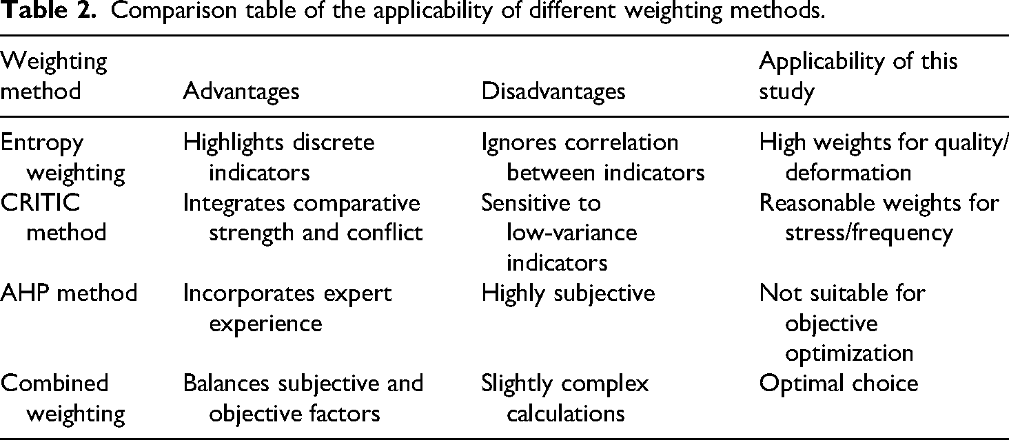
This article aims to objectively optimize the mechanical performance of the bed (static/dynamic characteristics, mass, stress) while minimizing subjectivity. The core reasons for choosing the CRITIC-entropy method are twofold:

The CRITIC-entropy method possesses complementary advantages. As shown in the table, entropy weighting excels in “highlighting discrete indicators"—which is crucial given the significant variability in deformation, frequency, stress, and mass indicators within our data set. Entropy captures the data-driven differences in these indicators, ensuring that the weights reflect the objective dispersion of the data. The CRITIC-entropy method integrates the comparative strength and conflicts among indicators. In this study, the indicators of deformation and natural frequency are interrelated. CRITIC balances these relationships, avoiding the overemphasis on a single indicator.

It mitigates the limitations of a singular approach. The standalone entropy method overlooks the correlations between indicators, a gap addressed by CRITIC, which analyzes conflicts among indicators. Conversely, CRITIC is “sensitive” to low-variance indicators, while entropy addresses this issue by focusing on data dispersion. Therefore, the combination of both methods ensures a balance and objectivity in the weightings for multiobjective optimization.

Compared to the AHP method, which incorporates expert experience but is highly subjective, this article prioritizes objective optimization to avoid bias in the weight distribution of quality, deformation, frequency, etc. The CRITIC-entropy method, in contrast to standalone entropy or CRITIC, overcomes the issue of ignoring correlations between indicators in the individual entropy method, while CRITIC addresses this concern. Standalone CRITIC performs poorly with low-variance indicators, whereas entropy tackles this through data dispersion. Consequently, the combined approach compensates for the individual shortcomings, ensuring the robustness of multiobjective weight calculations.

The CRITIC method, proposed by Diakoulaki et al. in 1995, is an objective weighting method that determines the objective weights of indicators by evaluating their contrast intensity and conflict. ³¹ The standard deviation represents the contrast intensity, while the correlation coefficient measures the conflict. The CRITIC method effectively considers both the contrast intensity and conflict among indicators. However, it does not fully account for the degree of dispersion among the indicators, which is where the entropy weight method comes into play by using the dispersion among indicators to determine weights.

By combining the CRITIC method and the entropy weight method, one can achieve a more comprehensive and objective reflection of the indicators’ weights. Therefore, this study opts to apply the combined CRITIC-entropy weight method to calculate the weights of indicators, aiming to reflect the characteristics and relationships within the data more accurately. This integrated approach leverages the strengths of both techniques, providing a balanced assessment of indicator importance.

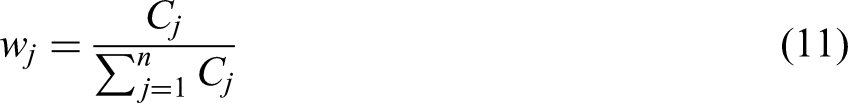
Weights are calculated based on the CRITIC method:

Constructing the decision matrix. Construct the decision matrix. When there are m models a₁，a₂，…a_i where i = 1，2，…m, and each model has n evaluation criteria denoted as a_i1， a_i2， … a_ij where j = 1，2，…n, the constructed matrix A can be represented as follows.

$$A={\left(\begin{array}{c}{\mathbf{a}}_{ij}\end{array}\right)}_{m\times \mathrm{n}}=\left[\begin{array}{cccc}{\mathbf{a}}_{11}& {\mathbf{a}}_{12}& \cdots & {\mathbf{a}}_{1j}\\ {\mathbf{a}}_{21}& {\mathbf{a}}_{22}& \cdots & {\mathbf{a}}_{2j}\\ ⋮& ⋮& ⋮& ⋮\\ {\mathbf{a}}_{i1}& {\mathbf{a}}_{i2}& \cdots & {\mathbf{a}}_{ij}\end{array}\right]$$

(5)

Standardization of evaluation criteria. The decision matrix A contains various evaluation criteria, which can be categorized into four types: maximization criteria, minimization criteria, intermediate criteria, and interval criteria. Maximization criteria imply that larger values, such as the first-order natural frequency, are preferable. Conversely, minimization criteria indicate that smaller values are desirable, exemplified by parameters like mass, maximum stress, and maximum strain. Therefore, it is necessary to standardize the evaluation criteria within the matrix A.

$$x_i={\displaystyle \frac{x_i-x_{\min }}{x_{\max }-x_{\min }}}$$

(6)

$$x_i={\displaystyle \frac{x_{\max }-x_i}{x_{\max }-x_{\min }}}$$

(7)

Calculate the contrast intensity of the jth index

$${\sigma }_j=\sqrt{{\displaystyle \frac{{\sum }_{i=1}^m(x_{ij}^{{}^{\mathrm{\prime }}}-{\overline{x}}_j^{{}^{\mathrm{\prime }}})}{m-1}}}$$

(8)

Calculate the conflict between evaluation indicators

The conflict reflects the degree of correlation among different criteria. A significant correlation indicates that the conflict value is smaller. Let the conflict level between criterion i and the remaining criteria be denoted as f, representing the conflict among the requirements.

$$f_j=\sum _{i=1}^m(1-r_{ij})$$

(9)

In the formula, r denotes the correlation coefficient between indicators i and j; the Pearson correlation coefficient is used here.

Calculate the information carrying capacity.

$$C_j={\sigma }_j{f}_j$$

(10)

The weights are calculated by fomula (11).

$$w_j={\displaystyle \frac{C_j}{{\sum }_{j=1}^n{C}_j}}$$

(11)

Weights are calculated based on the entropy weight method:

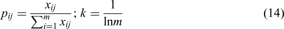
Standardization of indicators. This process aligns with step (2) of the CRITIC method.

Normalization of the decision matrix. The model optimized using the entropy weight method encompasses a variety of evaluation indicators. Due to potential discrepancies in units and magnitudes of these indicators, errors may arise in the computational results. Therefore, performing normalization calculations to derive the standardized decision matrix B is essential.

$$b_{ij}=\frac{a_{ij}}{\sqrt{{\sum }_{i=1}^m{a}_{ij}^2}}$$

(12)

Calculation of entropy values. A smaller entropy value for an indicator indicates that it provides more information, suggesting its higher importance and, consequently, a more significant weight. The calculation of the entropy value is as follows.

$$H_j=-k\sum _{i=1}^m(p_{ij}\ln p_{ij})$$

(13)

$$p_{ij}={\displaystyle \frac{x_{ij}}{{\sum }_{i=1}^m{x}_{ij}};k={\displaystyle \frac{1}{\ln m}}}$$

(14)

The calculation of the weights for each evaluation indicator in the system is as follows.

$$\begin{array}{rl}& {\omega }_j={\displaystyle \frac{1-{\mathbf{H}}_j}{{\sum }_{j=1}^n(1-{\mathbf{H}}_j)}}\\ & {\omega }_j\subset [0,1]\end{array}$$

(15)

Comprehensive weight calculation: The weight calculated using the CRITIC method is denoted as ${\omega }_c$ , and the weight calculated using the entropy method is denoted as ${\omega }_e$ . Therefore, the combined weight is as follows.

$$\omega ={\displaystyle \frac{1}{2}({\omega }_c+{\omega }_e)}$$

(16)

Comprehensive performance optimization model based on constraints

The model should minimize the objective function while satisfying the constraints. The constraints include the mass, maximum stress, and maximum strain being less than their initial values, the first-order natural frequency being more significant than the excitation frequency, and the dimensional parameters being within the specified range. Therefore, the comprehensive performance optimization model for the cross-bracing structure is as follows.

$$\{\begin{array}{cc}\min Y=w_M{Y}_M+w_{{\sigma }_{\max }}{Y}_{{\sigma }_{\max }}+w_{{\delta }_{\max }}{Y}_{{\delta }_{\max }}+w_{f_1}{Y}_{f_1}& \\ \mathrm{s}.\mathrm{t}.\{\begin{array}{cc}{Y}_{\mathrm{M}}\le M_0& \\ Y_{{\sigma }_{\max }}\le {\sigma }_0& \\ Y_{{\delta }_{\max }}\le {\delta }_0& \\ Y_{f_1}>{\displaystyle \frac{n}{60}}& \\ x_{i_{\min }}\le x_i\le x_{i_{\max }}& \end{array}& \end{array}$$

(17)

Modal experimental method

To verify the accuracy of the ANSYS simulation software results, a force hammer impact modal test was conducted on the machine tool bed. The first to sixth natural frequencies were obtained through experiments and compared with the ANSYS software simulation results to verify the reliability of the finite element simulation modeling and analysis method.

This article uses the Siemens LMS modal testing system to perform modal testing on the machine tool worktable and machine tool base. Before the test begins, a model point line diagram of the test component is established, and one point is selected as the test point for hammering. The X, Y, and Z directions of the excitation point are tapped separately to collect its excitation signal. The collected experimental data is processed and analyzed using Test lab software to measure the natural frequency of the machine tool component. The reliability of the measured modal data is expressed using a modal assurance criterion (MAC) diagram.

The equipment required for modal testing includes a force hammer, 356A16 ICP accelerometer, and SCM2E02 data collector. The modal testing equipment is shown in Figure 4. The parameters of the experimental equipment are shown in Table 3.

Figure 4.

Modal test equipment. (a) SCM2E02 data acquisition system; (b) 356A16 ICP three-way acceleration sensor; and (c) the Force hammer.

Table 3.

Acceleration sensor and force hammer parameters.

Name	Sensor serial number	Sensitivity
		X-direction(mV/g)	Y-direction(mV/g)	Z-direction(mV/g)
Sensor 1	LW258627	101.3	104.7	103.2
Sensor 2	LW258961	101.9	96.4	95.1
Sensor 3	LW258732	96.3	95.2	97.6
Sensor 4	LW258960	99.9	99.9	95.1
Sensor 5	LW258733	100.6	97.2	97.2
Hammer	20712	0.23 mV/N

This article uses the mobile sensor method to conduct modal tests on the bed structure. The function of the sensor in Figure 4 is to measure the dynamic response of the bed structure under excitation (such as acceleration, velocity, or displacement). Sensors move between different measuring points, collect vibration response data from each point, and construct the overall modal information of the bed structure. The function of a force hammer is to provide transient excitation (pulse force) and excite the vibration of the structure. A force hammer usually has a built-in force sensor that measures the magnitude and duration of the input force. By tapping the structure at fixed excitation points (such as single point excitation), the consistency of each excitation is ensured, facilitating subsequent frequency response function calculations. The function of the data collector is to synchronously collect the input force signal of the force hammer and the response signal of the sensor. Record time-domain data and convert it into frequency-domain data (such as frequency response function) through Fourier transform. Ensuring phase consistency of multichannel data is crucial for modal analysis.

Optimization algorithm for a machine bed structure

Simulated annealing algorithm

The SA algorithm is an approximate optimization technique based on the Monte Carlo method, designed to identify the optimal solution to a given problem. By emulating the annealing procedure, the algorithm initiates at a high temperature and progressively reduces it. This gradual cooling is paired with probabilistic jumps within the solution space to search for the optimal solution. ³² Consequently, SA can escape local optima with a certain probability when encountering suboptimal solutions, ultimately converging toward the global optimum, the approach of which effectively balances exploration and exploitation, enhancing the algorithm's ability to navigate complex solution landscapes.

The algorithm typically involves two levels of loops: an outer loop and an inner loop. The outer loop is responsible for gradually decreasing the temperature, while the inner loop performs multiple perturbations at the current temperature to generate different states. Through this mechanism, the simulated annealing algorithm can effectively explore the solution space and largely avoid getting trapped in local optima. This ability to probabilistically accept worse solutions at higher temperatures allows it to thoroughly search the solution space and improve the chances of finding a global optimum. The flow chart of SA is shown in Figure 2.

The acceptance of a new state in the inner loop follows the Metropolis criterion, whereby the probability of a particle achieving equilibrium at temperature T is given by $e^{-\frac{\mathrm{\Delta }E}{kT}}$ , where E denotes the internal energy at temperature T, ΔE the change in energy, and k the Boltzmann constant. The Metropolis criterion is commonly expressed as follows.

$$p=\{\begin{array}{c}{\mathrm{e}}^{-\frac{E(X_n)-E(X_0)}{T}},E(X_n)>E(X_0)\\ 1,E(X_n)\le E(X_0)\end{array}$$

(18)

In this context, X_n refers to the state at the subsequent time step, while X₀ the state at the preceding time step. E(X_n) represents the internal energy at the state X_n, and E(X₀) indicates the internal energy at the state X₀. The variable T signifies the temperature at the current time step. In the simulated annealing algorithm, the temperature T is reduced systematically, as illustrated by the following equation.

$$T(t)=\alpha T(t-1)$$

(19)

In this context, $\alpha$ is a constant slightly <1, referred to as the cooling coefficient, which takes values within the 0.85 <α< 1 range. The variable t denotes the iteration count.

The simulated annealing algorithm strongly depends on these two parameters: the initial temperature and the cooling coefficient. The appropriateness of selecting these parameters directly impacts the algorithm's performance. The flowchart of the SA algorithm is shown in Figure 5.

Figure 5.

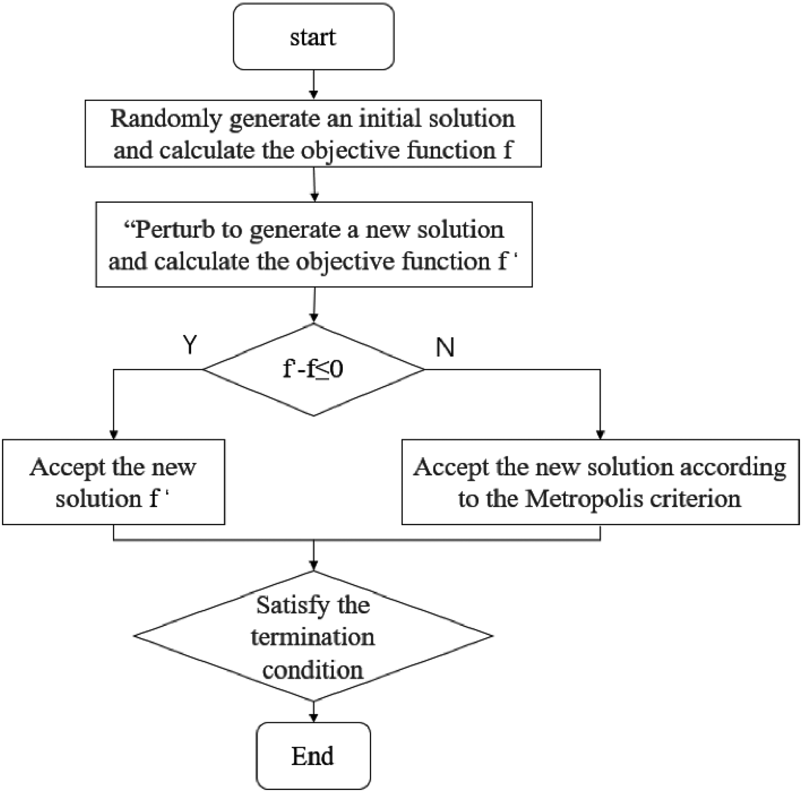
The flow chart of the simulated annealing (SA) algorithm.

Genetic algorithms

GA is a search and optimization algorithm based on the genetic evolutionary mechanisms observed in natural populations. It was first proposed by the American scholar John Holland in 1975. Genetic algorithms simulate the “survival of the fittest” principle in biological evolution, leading to progressively better populations through successive generations. ³³ The genetic operations involve three fundamental operators: selection, crossover, and mutation. These operators work on the individuals in a population based on their fitness values to perform operations akin to natural selection, crossover (recombination of genetic material), and mutation (random changes). The goal is to emulate the natural evolutionary process where the fittest individuals are more likely to survive and reproduce, thereby driving the evolution of the population toward optimal solutions. Through the iterative application of these operators, genetic algorithms effectively explore the search space and converge toward high-quality solutions.

The algorithmic workflow is illustrated in Figure 6.

Figure 6.

The flow chart of the genetic algorithm (GA).

Particle swarm algorithm

PSO is a swarm intelligence optimization algorithm proposed by Kennedy and Eberhart in 1995. It is developed based on the simulation of bird flocking or fish schooling behavior. PSO is a population-based search algorithm in which individuals, called particles, move through the solution space to find optimal solutions by updating their positions based on their own experience and the experience of their neighbors.

The algorithm's simple structure and easy implementation make it widely applicable to various optimization problems. ³⁴ Each particle adjusts its trajectory toward its personal best position and the global best position found by the swarm, balancing exploration and exploitation of the search space. This collaborative behavior allows PSOs to search for optimal solutions in complex problem domains effectively.

The main workflow of the algorithm is illustrated in Figure 4, with the key steps described as follows:

Parameter initialization: Set the number of iterations T, population size H, individual learning factor c₁, and social learning factor c₂.

Initial swarm creation: Generate an initial swarm by randomly producing starting positions and velocities.

Fitness evaluation: Calculate the fitness of all particles in the swarm. For each particle, identify the local best solution within the population, devoured as $p_{kd}(t)$ .

Position and velocity update: Update the position x_kd(t + 1) and velocity v_kd(t + 1) at the next time step using the following equations.

$$\begin{array}{rl}{v}_{kd}(t+1)=& w{v}_{kd}(t)+c_1{r}_1(t)(p_{kd}(t)-x_{kd}(t))+c_2{r}_2(t)(g_d(t)-x_{kd}(t))\\ x_{kd}(t+1)=& x_{kd}(t)+v_{kd}(t+1)\end{array}$$

(20)

Global best update: Recalculate the updated fitness and compare it with the local best Pbest to update the global best value gbest, denoted as $g_d(t)$ .

Iteration: Repeat steps (3), (4), and (5) until the stopping criteria are met.

The flowchart of the PSO algorithm is shown in Figure 7.

Figure 7.

The flow chart of the particle swarm optimization (PSO) algorithm.

Results and discussion

Results and discussion of the original machine bed

Structural static analysis results and discussion of the original machine bed

The structural static analysis of the bed body was conducted based on the finite element static analysis method. The finite element model of the original bed body is shown in Figure 8.

Figure 8.

Finite-element model.

To verify the reliability of the finite element model, a mesh convergence analysis was conducted. Meshes with characteristic sizes of 40, 30, and 20 mm were set up, and the variations of maximum total deformation and maximum equivalent stress under different mesh sizes were compared, as shown in Table 4.

Table 4.

Comparison table of simulation results for different sized mesh beds.

Mesh size （mm）	Maximum total deformation(mm)	Maximum equivalent stress （MPa）
40	0.43211	14.862
30	0.46239	15.12
20	0.43707	17.258

As the number of mesh elements increased and the mesh size decreased, both the total deformation and maximum equivalent stress exhibited dynamic changes. When the mesh size was refined from 40 to 30 mm, the total deformation increased from 0.43211 to 0.46239 mm, and the maximum equivalent stress rose from 14.862 to 15.12 MPa. Further refinement to 20 mm resulted in a slight decrease in total deformation to 0.43707 mm, while the maximum equivalent stress increased to 17.258 MPa. When the mesh size was smaller than 30 mm, the variations in total deformation and maximum equivalent stress stabilized, indicating that the mesh convergence criteria were met.

Considering both computational efficiency and accuracy, a mesh size of 30 mm was selected as the converged mesh to ensure the reliability of the finite element analysis results.

The stress distribution of the bed body is illustrated in Figure 9, while the total deformation diagram is presented in Figure 10. From the stress distribution of the cross-bracing structure, it can be observed that the equivalent stress is concentrated in the areas of the bed body that bear the load, particularly at the rear guide rail, where the maximum stress value of 15.172 MPa is located, which is significantly lower than the yield strength of the material. The total deformation diagram of the bed body shows that the overall deformation is relatively small, with the maximum deformation concentrated at the rear end. The point of maximum deformation occurs on the side near the spindle, with a maximum deformation of 0.046239 mm.

Figure 9.

The stress distribution diagram resulting from the analysis.

Figure 10.

The total deformation diagram illustrating the deformations observed.

Modal analysis results and discussion of the original machine bed

A modal analysis of the original machine bed was performed using ANSYS Workbench. The modal calculations were conducted following the finite element modal analysis method. The fundamental natural frequency of the cross-bracing structure is presented in Table 5, and the first mode shape is illustrated in Figure 11.

Figure 11.

The modal of bed. (a) The first order; (b) the second order; (c) the third order; (d) the fourth order; (e) the fifth order; and (f) the sixth order.

Table 5.

Modal analysis results.

Modal	Natural frequency [Hz]	Mode shape
1	97.418	Bending along Y axis
2	149.961	Bending along X axis
3	163.966	Twisting around Z axis
4	295.457	Bending and twisting
5	366.646	Bending and twisting
6	385.547	Bending along Y axis

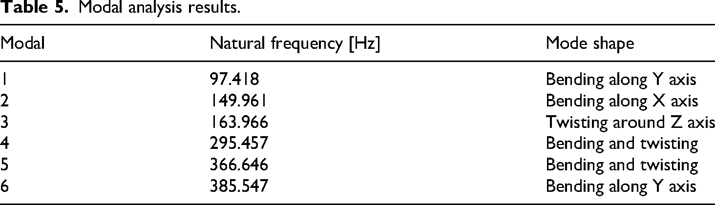
The modal simulation results are shown in Table 5.

As indicated in Table 5, the machine bed's fundamental natural frequency is 97.418 Hz, significantly higher than the external excitation frequency of 33.3 Hz. Figure 8 illustrates that the first mode shape exhibits bending along the Y-axis, with the maximum deformation concentrated in the middle region of the machine bed. The modal analysis results demonstrate that the original machine bed possesses good vibration resistance, allowing the setting of the first natural frequency to be a constraint in the optimization design process.

Modal experiment results

In practical modal testing of engineering, mechanical structures need to undergo modal testing under unhampered conditions. However, due to the limitations of actual testing conditions, the modal testing in this article is conducted under constrained conditions. In order to ensure the accuracy of the modal testing results, the boundary conditions of the modal testing are the same as those of the finite element modal simulation analysis process. Establish a bed frame point line diagram model in Testlab software. A total of 144 test points were established in this modal testing experiment, as shown in Figure 12. Point E3 was selected as the excitation point for.

Figure 12.

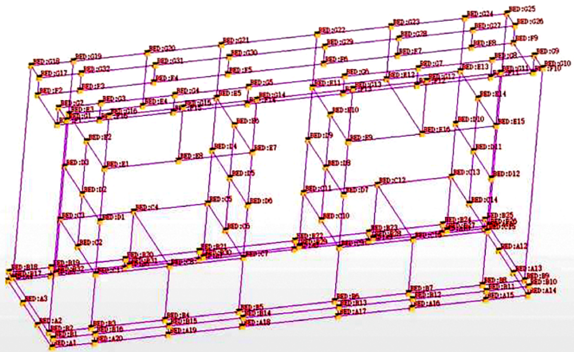
Dotted line plot of the experimental model.

This article uses MAC diagram to check the orthogonality of vibration modes and eliminate false models. The modal confidence criterion can check the orthogonality of the modal array. If the quality of the modal results is good, then in the MAC graph, the main diagonal element is 1 and the remaining elements are 0. The modal confidence criterion formula is shown in the formula.

$${\mathrm{MAC}}_{jlk}={\displaystyle \frac{{({\{R_{jk}\}}^{t*}\{R_{lk}\})}^2}{({\{R_{jk}\}}^{t*}\{R_{jk}\})({\{R_{lk}\}}^{t*}{\{R_{lk}\}}_s)}}$$

(21)

In formula (21), $R_{jk}$ and $R_{lk}$ are modal vectors. When there is a linear relationship between the two, its MAC value is 1; If there is no linear relationship between the two, their MAC values are close to 0.

The size of the MAC graph is usually used to determine the degree of correlation between modalities. An MAC value <0.05 indicates no correlation between modalities, while a value >0.9 indicates a high degree of correlation between modalities. The MAC diagram obtained from the modal test is shown in the Figure 13.

Figure 13.

The modal assurance criterion (MAC) diagram for model validation.

From the modal shape diagram of Figure 13, it can be seen that the main diagonal elements of the MAC diagram are all red, and the rest of the colors are blue or light blue, indicating that the state confidence standard of this experiment remains below 20%, and the frequency and formation obtained from the experiment are reasonable.

The comparison table between modal experimental results and modal simulation results is shown in Table 6.

Table 6.

Comparison table of modal experiment results and simulation results.

Order	First order	Second order	Third order	Fourth order	Fifth order	Sixth order
Simulation mode （HZ）	97.418	149.96	163.97	295.46	366.65	385.55
Experimental mode （HZ）	94.996	140.334	165.563	290.739	364.512	388.895
Error	2.4%	6.04%	0.9%	1.7%	0.5%	0.8%

From the comparison table of modal test results in Table 6, it can be seen that the error between the modal frequency obtained from the modal test and the modal frequency obtained from the finite element simulation is <7%. Within a reasonable error range, the accuracy of the finite element simulation model is verified, providing a theoretical basis for subsequent optimization of machine tool structures.

The effectiveness of the optimization in this study is validated through dual high-precision verification: first, static stiffness simulation shows that under the rated load, the maximum deformation of the optimized bed is reduced to 126.1 μm (a decrease of 9.41%), which is consistent with theoretical predictions; second, modal testing reveals that the error in the first six natural frequencies is  ≤ 7% with an MAC value  < 0.2, thereby indirectly validating the optimization effects and confirming the reliability of the dynamic characteristic modeling; however, practical cutting tests have not yet been conducted due to the high casting and assembly costs of the QLM27100-5x machining center and the excessively long required duration for comprehensive cutting performance testing; future work will integrate real cutting force measurements and machining accuracy assessments to validate the dynamic performance of the optimized bed.

Multiobjective optimization modeling of the machine bed

Preliminary selection of optimization parameters

Before implementing the lightweight design of the machine bed, it is essential to identify the optimization parameters. To reduce the computational workload during the finite element analysis process, dimensions that have a minimal impact on the mass of the machine bed were disregarded. Given the specific functional requirements of the machine bed within the gantry CNC machine, the length, width, and height must remain constant. A thin-walled structure characterizes the ribs and wall thickness of the machine bed, and variations in these dimensions significantly influence the mass of the machine bed. Consequently, the wall thickness W, rib thicknesses R₁ and R₂ in the XY and YZ directions, as well as the widths of the weight-reduction holes L₁, L₂, and L₃ in the ZX, YZ, and XY directions, are preliminarily established as design variables for the experimental setup, as illustrated in Figure 14.

Figure 14.

The schematic diagram of the bed configuration.

Determine the sensitivity analysis of design variables

To quantify the coupled effects of the bed's geometric parameters on multiobjective performance, this study employs sensitivity analysis to compare the influence of various design parameters on the performance of the bed. Using ANSYS Workbench software for the sensitivity analysis, the design dimensions of the bed are set as input parameters (design variables) with specified ranges of variation. The output parameters include the mass of the bed, maximum stress, maximum deformation, and the first natural frequency, allowing for an assessment of how changes in the input parameters affect the output parameters. The results are presented in Figure 15. The height of the bars in Figure 15 reflects the degree of influence that the dimensions have on the objectives; a greater height indicates a larger impact. The positive and negative values of the bars indicate whether the variables are positively or negatively correlated with the objectives.

Figure 15.

Sensitivity analysis of each objective. (a) Mass; (b) maximum stress; (c) maximum deformation; and (d) the first-order natural frequency.

From the sensitivity histogram in Figure 15, it is evident that W, R₁, R₂, and L₂ have a significant impact on the performance of the bed. For the mass of the bed, W, R₁, and R₂ exert a positive influence, while L₁, L₂, and L₃ have a negative influence. Regarding the maximum equivalent stress, W and R₂ have a negative impact, while R₁, L₁, L₂, and L₃ positively influence it. For the maximum deformation, L₂ and L₃ have a positive effect, whereas W, R₁, and R₂ exert a negative influence; L₁ has a minimal impact. In terms of the first natural frequency, W and R₂ positively affect it, while R₁ and L₂ have a negative influence, and L₁ and L₃ have little effect. By comparing the sensitivity of these six structural parameters on the bed's mass, maximum stress, maximum deformation, and first natural frequency, it is clear that the structural dimensions W, R₁, R₂, and L₂ significantly affect the performance indicators of the bed. Therefore, these four structural parameters are selected as optimization design variables, with their initial values and ranges specified in Table 7.

Table 7.

Range of bed design variables.

Design variables	Initial value (mm)	Minimum value (mm)	Maximum value (mm)
W	20	14	25
R1	20	14	25
R2	20	14	25
L2	180	165	205

DOE experimental design

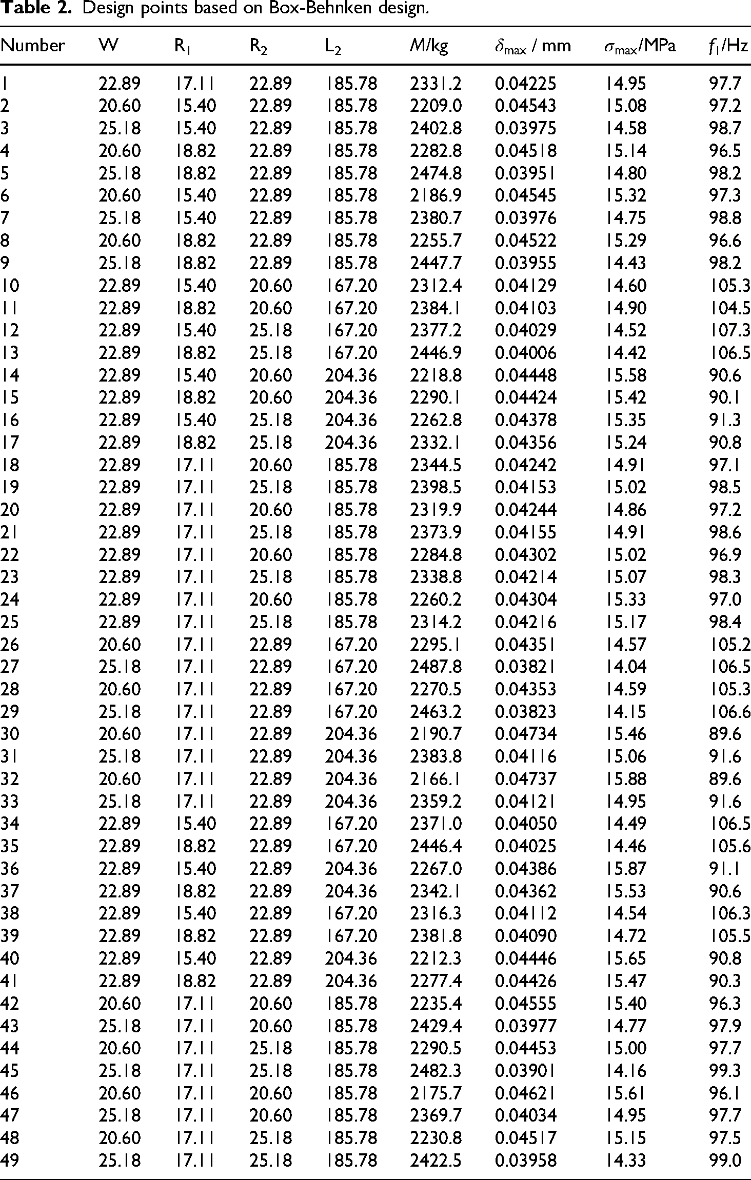
The design points for the machine bed were primarily generated using the RSM within the ANSYS software, explicitly employing the DOE approach. Three distinct experimental designs were utilized: CCD, BBD, and LHS. This process resulted in the acquisition of 45, 49, and 95 samples, respectively, leading to 189 samples, as presented in appendix.

Neural network fitting objective functions

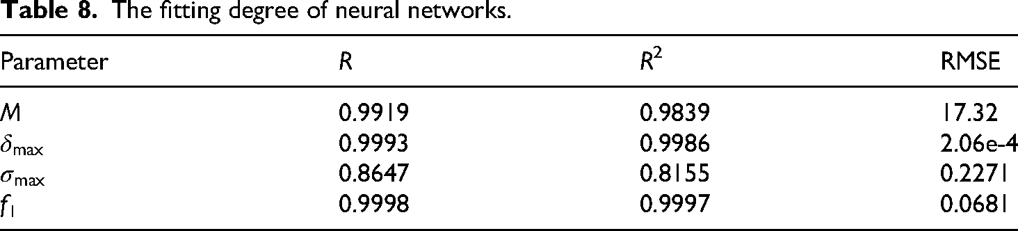
From the 189 data sets presented in the appendix table, 179 sets were selected for neural network fitting. Each target function was fitted separately, with each neural network comprising 4 input neurons, 1 output neuron, and 10 hidden layer nodes, as illustrated in Figure 16. The training process employed the Levenberg-Marquardt algorithm, utilizing 70% of the data as the training set, 15% as the validation, and 15% as the test set. As shown in Figure 17, the computational results between the fitted function model and the finite element analysis are very close, with the goodness of fit exceeding 0.74. The fitting accuracy of the neural network is presented in Table 8.

Figure 16.

The structure of the neutral network.

Figure 17.

Regression plot between outputs and targets. (a) Mass contrast; (b) the maximum stress contrast; (c) the maximum deformation contrast; and (d) the first-order natural frequency contrast.

Table 8.

The fitting degree of neural networks.

Parameter	R	R 2	RMSE
M	0.9919	0.9839	17.32
${\delta }_{\max }$	0.9993	0.9986	2.06e-4
${\sigma }_{\max }$	0.8647	0.8155	0.2271
f 1	0.9998	0.9997	0.0681

The error curves for the fittings are depicted in Figure 18. The remaining 10 datasets were used to compare the fitted values with those obtained from the finite element analysis, with the comparison results presented in Figure 19. Consequently, the fitting of each target function was successful, demonstrating the ability to effectively predict the values of each target under simulated experimental conditions.

Figure 18.

Fit error curve. (a) Mass contrast; (b) the maximum stress contrast; (c) the maximum deformation contrast; and (d) the first-order natural frequency contrast.

Figure 19.

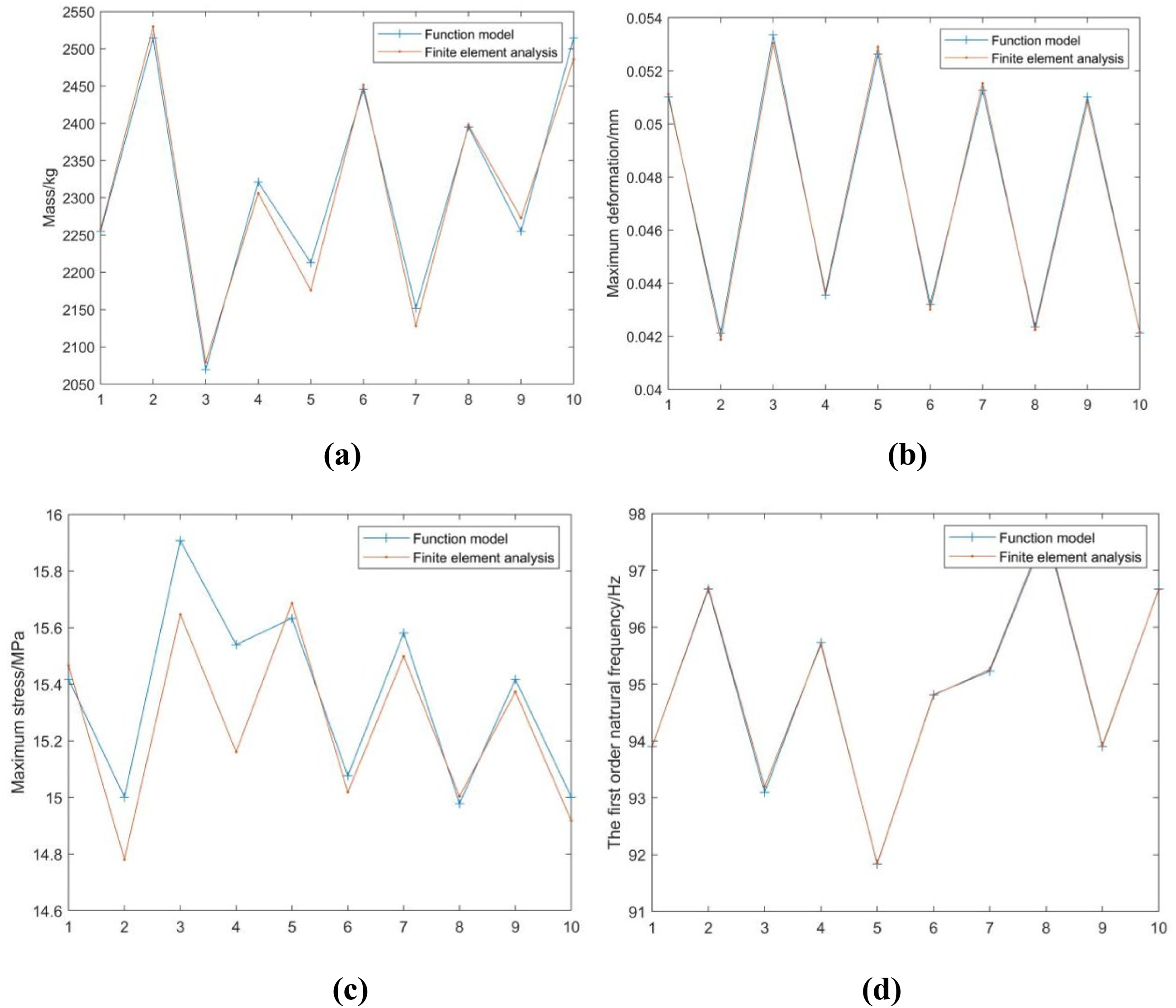
Comparison of calculation results. (a) Mass contrast, (b) the maximum stress contrast, (c) the maximum deformation contrast, and (d) the first-order natural frequency contrast.

Figure 20 illustrates the comparison between the predicted values and actual values of the fitting functions for the four optimization design objectives, showing that the predicted values (blue line) generally follow the trend of the actual values (black line), indicating that the neural network effectively captures the main variation patterns of the data for the four optimization design objectives, along with the 95% confidence interval.

Figure 20.

The comparison chart of the actual values and predicted values of the fitted function. (a) Predicted value and confidence interval of mass; (b) predicted value and confidence interval of deformation; (c) predicted value and confidence interval of stress; and (d) predicted value and confidence interval of the first order natural frequency.

As shown in Figure 20, the predicted values of the four optimized design objective fitting functions predominantly fall within the 95% confidence interval (pink area), which reflects the statistical reliability of the model predictions to some extent.

The residual plots of the fitting functions for the four optimized design objectives are shown in Figure 21.

Figure 21.

Residual plots for the predictions of the four optimization design objectives. (a) Residual plot of mass; (b) residual plot of deformation; (c) residual plot of stress; and (d) residual plot of the first order natural frequency.

The residuals fluctuate around the zero line (horizontal dashed line) without a discernible trend related to the sample index, indicating that the model's prediction errors do not exhibit systematic bias and largely align with the expected random distribution, reflecting the model's capability to capture data patterns to some extent.

Weight coefficients of each optimization objective

The entropy weight and CRITIC methods were employed to process the objective data, resulting in the weight coefficients for each optimization target, as derived from equation (16) and presented in Table 7. By substituting the initial values of the design variables into the fitted neural network functions, the following results were obtained: M₀ = 2241.0 kg, δ₀ = 0.0463 mm, σ₀ = 15.172 MPa, and f₁₀ = 97.4 Hz. Consequently, a comprehensive objective function for the optimization design of the machine bed was established.

$$Y=0.41925{\displaystyle \frac{Y_M-M_0}{M_0}+0.29265{\displaystyle \frac{Y_{{\delta }_{\max }}-{\delta }_0}{{\delta }_0}+0.1919{\displaystyle \frac{Y_{{\sigma }_{\max }}-{\sigma }_0}{{\sigma }_0}+0.0962{\displaystyle \frac{f_1-Y_{f_1}}{f_{10}}}}}}$$

(22)

The weight coefficient table for optimizing objectives is shown in Table 9.

Table 9.

Weight coefficients of optimization objectives.

parameter	M/kg	${\delta }_{\max }/\mathrm{mm}$	${\sigma }_{\max }$ /MPa	f1/Hz
Entropy weight method	0.4048	0.3185	0.2744	0.0023
CRITIC method	0.4337	0.2668	0.1094	0.1901
Average	0.41925	0.29265	0.1919	0.0962

Multiobjective optimization model

The optimization model is as follows.

$$\{\begin{array}{cc}\min Y=0.41925{\displaystyle \frac{Y_M-M_0}{M_0}+0.29265{\displaystyle \frac{Y_{{\delta }_{\max }}-{\delta }_0}{{\delta }_0}+0.1919{\displaystyle \frac{Y_{{\sigma }_{\max }}-{\sigma }_0}{{\sigma }_0}+0.0962{\displaystyle \frac{f_1-Y_{f_1}}{f_{10}}}}}}& \\ s.t.\{\begin{array}{cc}{Y}_M<2241.0& \\ Y_{{\delta }_{\max }}\le 0.0463& \\ Y_{{\sigma }_{\max }}\le 15.172& \\ Y_{{\int }_1}\ge 33.3& \\ 14\le x_1\le 20& \\ 14\le x_2\le 20& \\ 14\le x_3\le 20& \\ 165\le x_3\le 205& \end{array}& \end{array}$$

(23)

Optimization results and discussion of machine bed

Model solving based on the SA algorithm

The multiobjective optimization model for the machine bed was solved using the SA algorithm implemented in MATLAB software. Testing indicated that the algorithm began to converge around T = 11. To achieve a better global optimum solution while minimizing computational time, we set the maximum number of iterations to T = 50. The initial temperature was set at T0 = 100, with L = 100 iterations per temperature level and a temperature decay coefficient of α = 0.95. The optimization model was solved according to the algorithmic flow outlined in Figure 5. The optimal solutions are presented in Table 10, while the convergence plot of the algorithm is shown in Figure 22. It can be observed from the figure that the algorithm exhibits a rapid convergence rate, with a total computation time of 12.7 seconds.

Figure 22.

Convergence diagram of the algorithm solution.

Table 10.

Algorithm solution results.

Variables	W (mm)	R1 (mm)	R2 (mm)	L2 (mm)
Optimization results	23.81	14.0	14.007	165.00

Model solving based on Ga algorithm

The multiobjective optimization model for the machine bed was solved using a GA implemented in MATLAB software. Testing revealed that the algorithm began to converge around T = 13. To achieve a more optimal global solution while reducing computational time, we set the maximum number of iterations to T = 50. The population size was N = 100, with a mutation probability P_c of 0.2 and a crossover probability P_m of 0.2. The optimization model was solved according to the algorithmic flow illustrated in Figure 6. The optimal solutions are presented in Table 11, while the convergence plot of the algorithm is depicted in Figure 23. It can be observed from the figure that the algorithm demonstrates a rapid convergence rate, with a total computation time of 5.84 seconds.

Figure 23.

Convergence diagram of the algorithm solution.

Table 11.

Algorithm solution results.

Variables	W (mm)	R1 (mm)	R2 (mm)	L2 (mm)
Optimization results	23.85	14.00	14.00	165.00

Model solving based on PSO algorithm

The multiobjective optimization model for the machine bed was solved using a PSO algorithm implemented in MATLAB software. Testing indicated that the algorithm began to converge at approximately T = 9. We set the maximum number of iterations to T = 50 to enhance the global optimal solution while minimizing computational time. The individual learning factors c1 and social learning factors c2 were set to 2.05. The maximum inertia weight ${\omega }_{\max }$ was specified as 0.9, while the minimum inertia weight ${\omega }_{\min }$ was set at 0.4. The maximum convergence speed was determined to be 1/8 of the range of the variable values. The number of particles in the swarm (H) was typically between 20 and 40; for most scenarios, 30 particles yield satisfactory results. Thus, we selected H = 30. Following the algorithmic flow presented in Figure 7, we solved the optimization model. After parameter configuration, the dimensions of the machine bed were initialized randomly, and the comprehensive objective function was computed to obtain the function value. Subsequently, the dimension variables were updated within the specified range, and the comprehensive objective function value was recalculated. The current historical optimal value was selected by comparing this value with the previous function value. The global optimal value was identified by continuously updating the dimension variables and comparing different function values. When the iteration termination conditions were met, the current historical optimal value represented the global optimal value, with the corresponding dimension variable values reflecting the optimal solution. The optimal solutions are summarized in Table 12, and the algorithm's convergence plot is illustrated in Figure 24. The Figure demonstrates that the algorithm converges rapidly, with a total computation time of 0.72 seconds.

Figure 24.

Convergence diagram of the algorithm solution.

Table 12.

Algorithm solution results.

Variables	W (mm)	R1 (mm)	R2 (mm)	L2 (mm)
Optimization results	23.85	14.00	14.00	165.00

Comparison of optimization effects of various algorithms

The parameters of the three optimization algorithms are shown in the Table 13.

Table 13.

Optimization algorithm parameters.

Optimization algorithm	Parameter	Value
Simulated annealing	Initial temperature （T0）	100
	Cooling rate （α）	0.95
	Maximum iterations （T）	50
	Iterations per temperature level （L）	100
Genetic algorithm	Population size （N）	100
	Crossover probability （Pm）	0.2
	Mutation probability （Pc）	0.2
	Maximum iterations （T）	50
Particle swarm optimization	Number of particles （30）	30
	Individual learning coefficient （C1）	2.05
	Social learning coefficient （C2）	2.05
	Inertia weight （ω）	0.4–0.9
	Maximum iterations （T）	50

Comparison table of calculation time and iteration times for three algorithms, as shown in Table 14.

Table 14.

Comparison of calculation time and iteration counts for three algorithms.

Optimization algorithm	Calculation time (s)	Convergent iteration counts
SA	12.7	11
GA	5.84	13
PSO	0.72	9

As shown in the table above, the PSO algorithm demonstrates a significant advantage in time efficiency. Its population-based collaborative search mechanism avoids the progressive cooling process required by the SA algorithm, while also circumventing the computational overhead associated with the complex crossover and mutation operations in the GA algorithm. Although all three algorithms are set to a maximum of 50 iterations, PSO achieves a stable solution by the 9th iteration, indicating its superior applicability in the optimization of machine tool structures.

Comparative analysis and discussion of pre- and postoptimization

The results obtained by the algorithm are rounded, and two decimal places are retained. The modified machine bed model was then imported into ANSYS Workbench for dynamic and static performance analysis, yielding the optimization results. These results are presented in Table 15.

Table 15.

Comparison results.

Parameters	W (mm)	R1 (mm)	R2 (mm)	L2 (mm)	M/kg	${\delta }_{\max }/\mathrm{mm}$	${\sigma }_{\max }$ /MPa	f1/Hz
Before optimization	20	20	20	180	2242.5	0.04623	15.172	97.4
After optimization	23.85	14.00	14.00	165.00	2228.1	0.04188	14.985	103.0
Change rate	19.25%	−30.00%	−30.00%	−8.33%	−0.64%	−9.41%	−1.23%	5.75%

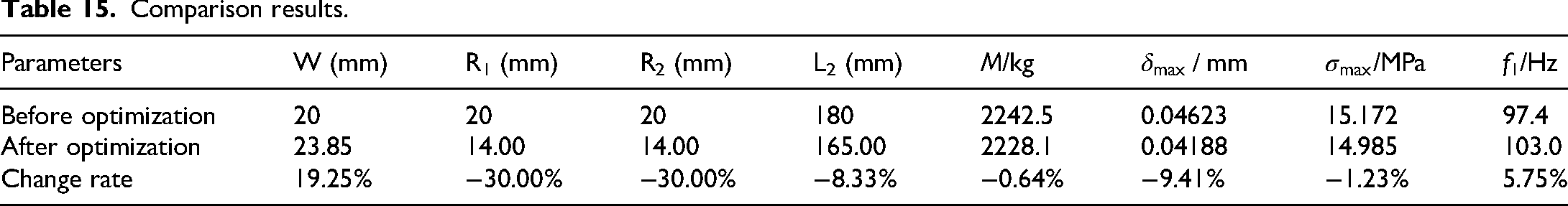
Figure 25 illustrates the optimized machine bed's stress distribution, total deformation, and first-order mode shape.

Figure 25.

Dynamic and static performance of bed after comprehensive optimization. (a) Stress, (b) total deformation, and (c) the first-order modal shape.

The comparison table of the bed performance before and after optimization is shown in Table 16.

Table 16.

Comparison of bed performance before and after optimization.

Indicator	Before optimization	After optimization	Change amount
Maximum deformation (mm)	0.0462	0.0418	−9.41%
Mass (kg)	2242.5	2228.1	−0.64%
Maximum equivalent stress (MPa)	15.17	14.95	−1.23%
First natural frequency (Hz)	97.418	103.04	+5.75%

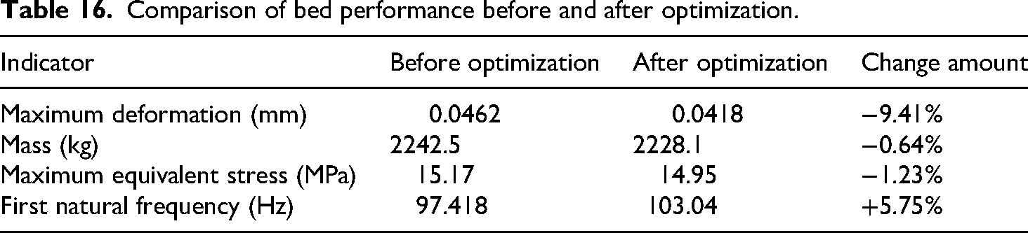
The comparative analysis of performance metrics before and after optimization revealed that the maximum deformation of the optimized machine bed structure was reduced by 9.41%, the first-order frequency increased by 5.75%, the maximum stress decreased by 1.23%, and the mass was reduced by 0.64%. The optimization design presented in this study effectively minimized the maximum deformation of the machine bed, thereby enhancing machining accuracy and improving overall processing quality.

From the preceding analysis, it is evident that the optimized machine bed's mass remained unchanged, while the maximum stress was reduced and the first-order frequency increased, demonstrating significant improvements in maximum deformation. This indicates that, under the condition of relatively constant mass, the dynamic and static performance of the machine bed was maximally enhanced. Thus, this study's lightweight design optimization approach proved practical and feasible.

Conclusion

This article investigates a multiobjective optimization design method for the structure of a gantry machining center's machine bed, aimed at optimizing its structural design across multiple targets. Sensitivity analysis was conducted to identify key structural parameters that significantly impact the performance of the machine bed, with these parameters selected as the focus of optimization—design of Experiments DOE was employed to analyze the machine bed's dimensions further. Based on the results of the DOE analysis, mathematical models for each optimization objective were fitted using response surface methodology and neural network techniques. At the same time, the entropy weight method was utilized to allocate weights to the optimization objectives. Subsequently, a comprehensive optimization model aimed at enhancing the dynamic and static characteristics of the machine bed was constructed. Solutions were derived using intelligent algorithms such as SA, GA, and PSO through MATLAB software. The results demonstrated that the maximum deformation of the optimized machine bed was significantly reduced, the maximum stress was lowered, and the first-order natural frequency was increased. At the same time, the mass of the machine bed was also decreased. Overall, the dynamic and static performance showed notable improvements. Therefore, this optimization method provides a practical and effective solution for the lightweight design of the machine bed.

This study presents a lightweight multiobjective optimization method based on hybrid experimental design, neural network models, and a combination weighting PSO algorithm, which demonstrates good engineering transferability and can be extended to similar gantry machine structures; however, targeted adjustments are necessary for practical applications. The core method is applicable to static beam and moving beam gantry machines, as well as other symmetrical topologies, such as double-column turning-milling composite centers. In cases where there is a significant frequency difference between the workpiece-tool system, such as in heavy cutting machine tools, frequency thresholds need to be recalibrated based on impact testing. The limitation of this method is that it is not suitable for asymmetric structures, such as C-type column machining centers, due to uneven rigidity distribution leading to ineffective sensitivity analysis.