Sage Journals: Discover world-class research

Abstract

Fault diagnosis technologies for ocean-going marine diesel engines play an important role in the safety and reliability of ship navigation. Although many fault diagnosis technologies have achieved acceptable results for single fault of diesel engines, the diagnosis of multiple faults is rarely involved. Due to the strong correlation, non-linearity and randomness of multiple faults, it is extremely difficult to make an accurate diagnosis. In this study, diagnosis methods based on thermal parametric analysis combined with different neural network algorithms were established and used for the diagnosis of multiple faults in the ocean-going marine diesel engine. The results show that the Levenberg Marquardt back propagation neural network has the highest diagnostic accuracy rate of 88.89% and 100% for multiple faults and single faults, respectively, and its diagnostic time is also relatively short, 0.78 s. The Bayesian regularization back propagation neural network can give a diagnostic accuracy rate of 100% for single faults, but for multiple faults, the diagnostic accuracy rate is only 55.56%, and the diagnosis time for the entire sample is the longest. As for the probabilistic neural network, although it has the fastest diagnosis speed, it has the lowest diagnostic accuracy rate for both single faults and multiple faults. The results may provide references for the online diagnosis of single faults and multiple faults in ocean-going marine diesel engines.

Keywords

Marine diesel engine multiple faults diagnosis neural network Levenberg Marquardt back propagation neural network Bayesian regularization back propagation neural network probabilistic neural network

Introduction

Large two-stroke marine diesel engines are the main power plant of ocean-going ships, which have the characteristics of long working hours and harsh working conditions. The health status of the engine has an important impact on the ship’s safety and cargo transportation timeliness. Therefore, real-time monitoring and diagnosing of the faults existing on the ocean-going marine diesel engine is of great significance.

There are multiple systems included in ocean-going marine diesel engines, such as turbocharger systems, air intake and intercooling systems, fuel injection systems, exhaust valve control systems and so on. It is a whole of multiple systems working together. In the long working process of marine diesel engines, the failure of one system may cause a chain reaction and cause a failure of other systems. In addition, multiple systems may fail at the same time. Therefore, the situation of multiple faults occurring at the same time exists in a real marine diesel engine. The multiple faults of marine diesel engines not only have strong randomness when they occur, but also have strong correlation and non-linearity among them. Therefore, it is difficult to diagnose the multiple faults accurately.

For diesel engine fault diagnosis, there are three traditional diagnostic technologies including oil analysis technology,¹ vibration analysis technology,² and thermal parametric analysis technology,³ as shown in Figure 1. Oil analysis technology is used to detect the quality of lubricating oil in the crankcase of a diesel engine, which can diagnose the wear fault of moving parts. Sala et al.⁴ analyzed the lubricating oil of a diesel engine and confirmed that the lubricating oil analysis method has a good diagnostic performance for the wear fault of diesel engines. However, due to the high price of oil detection equipment and the long detecting time, it cannot be carried out on ships. Vibration analysis technology which has strong fault diagnostic capacity collects vibration signals by installing sensors in the specific position of diesel engines. Many experimental results show that the vibration analysis method has a high diagnostic accuracy rate for excessive valve clearance, fuel system faults and so on.^5–8 However, this diagnostic method often requires the installation of a large number of sensors. Meanwhile, the vibration signal acquisition process is easily affected by other interference sources. Those shortcomings increase the cost of the ship construction and the complexity of the control system. The thermal parametric analysis technique diagnoses the fault by collecting and analyzing the thermal parameters during the working process of the engine. This method needs a few thermal parameters, which can be collected directly or indirectly through the cylinder pressure sensor. Many experimental results have verified that the faults can be accurately diagnosed by reasonable analysis of the thermal parameters.^9–12 Due to the high price and relatively low reliability of the cylinder pressure sensor, this method is mostly used in laboratories. However, the existing studies on the diagnosis of diesel engine faults based on the three traditional diagnostic technologies have not involved multiple faults, and there is still a lack of relevant literature for reference.

Figure 1.

Traditional diagnostic methods occur at the same time exist in daily life.

With the development of artificial intelligence, which has been applied to various fields. It is no exception in terms of diesel engine fault diagnosis. Xu et al.¹³ proposed a multi-model fusion system based on the evidential reasoning rule. The results showed that the system can accurately diagnose the wear faults of diesel engines including adhesive wear, abrasive wear and so on. Compared with the single data-driven diagnostic model, the proposed fusion system has a more accurate rate and robust ability. Jafarian et al.¹⁴ used the Fourier transform to extract features of vibration signals from diesel engines. The artificial neural networks, support vector machine and K-nearest neighbour algorithm were used to diagnose the fault of a misfire, and valve clearance and to predict the health state of the engine. The research showed that the support vector machine has higher accuracy than the K-nearest neighbour algorithm and artificial neural network. Nahim et al.¹⁵ used a decision tree as a diagnosis tool to diagnose the fault of misfires in internal combustion engines. They separated samples of vibration signals into the training database and testing database. The training database was used to establish the classification model and the testing database was used to verify the accuracy of the classification model. The research showed that the accuracy of the decision tree at 1000 and 1500 r/min is 94.6% and 95.3%, but the accuracy of the classifier is 68% at 2000 r/min, which can be explained to the sudden appearance of very strong vibrations muffling the misfire knock signal. Cao et al.¹⁶ used the K-means algorithm to analyse the data and created a BP (back propagation) neural network to diagnose the fault of a diesel engine. The faults include injector needle valve wear, exhaust valve leakage and piston ring wear. The results showed that the diagnostic accuracy rate of this method could reach 91.4%, which implied the good performance of the combination of K-means and BP neural network. In general, the diagnosis methods mentioned above have achieved high accuracy and performance. However, almost all types of faults in the above studies were also single fault and no multiple faults were taken into consideration.

Since cylinder pressure sensors are more and more commonly installed in ocean-going marine diesel engines, it is possible to diagnose faults in this type of engine based on thermal parametric analysis technology. Then the installation of a large number of additional sensors can be reduced or even avoided. Considering the non-linearity of multiple faults and the advantages of neural networks in dealing with nonlinear problems, this study attempts to use thermal parametric analysis combined with different neural network algorithms to diagnose the multiple faults of the ocean-going marine diesel engines to evaluate the diagnostic effects and provide references for practical application. Levenberg Marquardt (LM) algorithm and Bayesian regularized (BR) algorithm, which may eliminate the shortcomings of BP neural network¹⁷ and improve the accuracy of fault diagnosis,¹⁸ and a probabilistic neural network (PNN) are introduced. The three different neural network algorithms are established and used to diagnose the single and multiple faults of the ocean-going marine diesel engines based on the thermal parameters in this study. This may provide a novel perspective for the multiple fault diagnosis of ocean-going marine diesel engines.

Selection of diesel engine failure

Due to the huge size and complexity of the mechanical system, it is difficult to carry out experiments on ocean-going marine diesel engines. At the same time, considering the irreversible damage and immeasurable loss that may be caused after the fault occurs, a simulation model based on thermodynamics that can simulate the entire working process of the ocean-going marine diesel engine is established in GT-Power software in this study, as shown in Figure 2.

Figure 2.

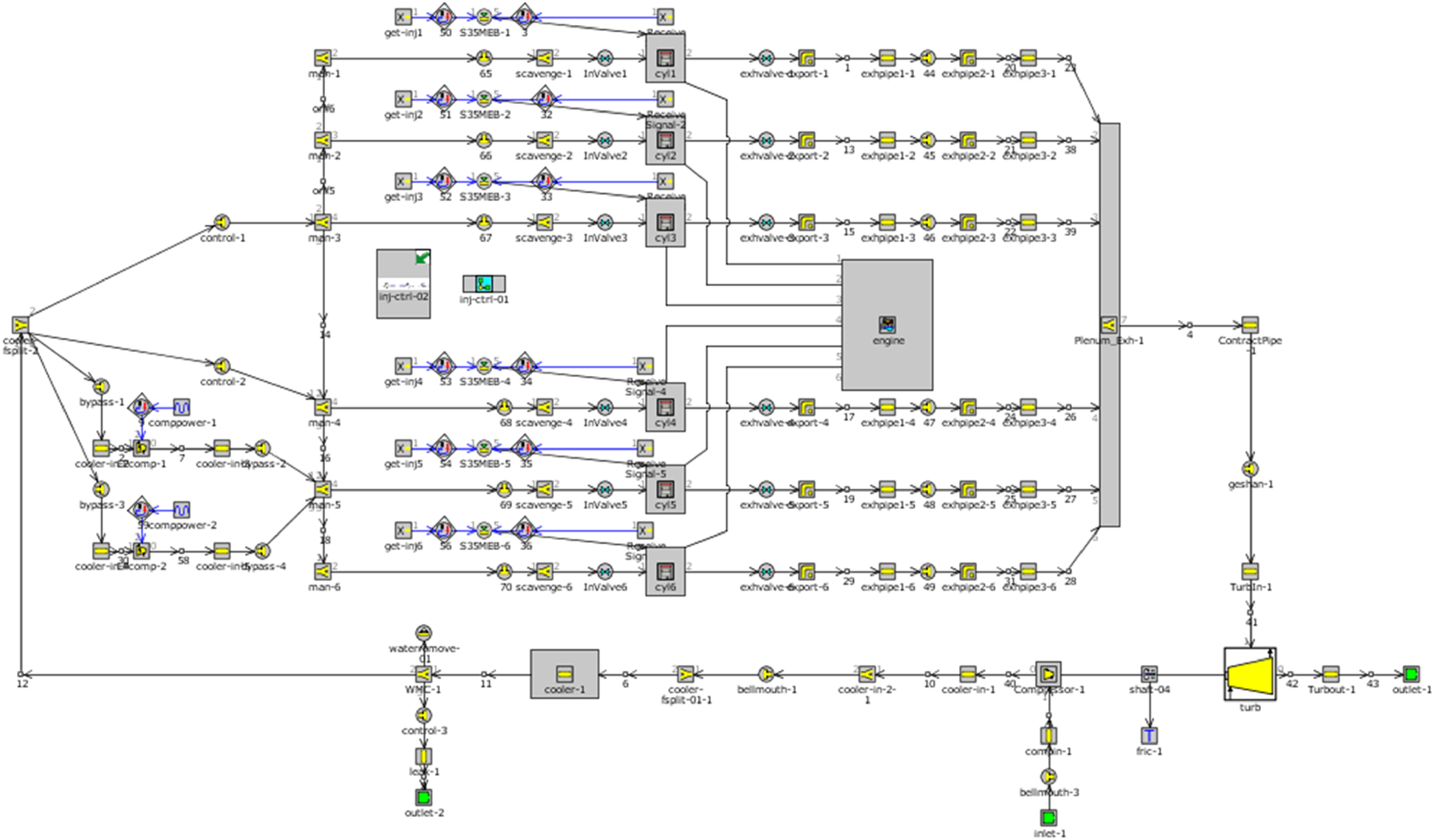
The simulation model was established in the GT-Power software.

Basic parameters of the marine diesel engine

The basic parameters of the ocean-going marine diesel engine used in this study are shown in Table 1. This type of diesel engine is a high-power low-speed marine diesel engine, which is independently developed and manufactured by China Shipbuilding Power Research Institute. It has passed the approval inspection of the China Classification Society (CCS). The physical map of the engine is shown in Figure 3.

Figure 3.

The physical map of the marine diesel engine.

Table 1.

Specifications of the marine diesel engine.

Parameter	Value
Engine type	Two-stroke, low-speed
Rated power, kW	4896
Rated revolution, r/min	157
Cylinder bore, mm	340
Stroke of cylinder, mm	1600
Connecting rod, mm	1600
Fuel injection system, –	Common rail
Type of fuel, –	Diesel oil/heavy oil

Characteristic parameters

The characteristic parameters selection is very important for the fault diagnosis. It has an important impact on the performance and accuracy of fault diagnosis. The principle of characteristic parameter selection is that the parameters can be easily obtained by existing sensors on the engine. Then the fault diagnostic system can be simplified. In this study, seven kinds of parameters, namely peak pressure of cylinder ( $P_{m a x}$ ), crank angle of the peak pressure ( $D_{m a x}$ ), indicated mean effective pressure ( $I M E P$ ), turbocharger inlet ( $T T_{e x h . i n}$ ) and outlet ( $T T_{e x h . o u t}$ ) exhaust temperature, in-cylinder pressure at 20 °CA before top dead center ( $P_{B 20}$ ) and fuel injection mass ( $F u e l_{i n j}$ ) are used as the characteristic parameters for fault diagnosis. These parameters can be easily obtained by cylinder pressure sensors and fuel flow rate sensors, which are more and more commonly installed on marine diesel engines. It should be noted that the $D_{m a x}$ can be obtained by the combination of crankshaft and camshaft position sensors which can encode the crankshaft angle and realize the control of fuel injection timing. In addition, temperature sensors of the turbocharger inlet and outlet have already been installed on the engine, so there is no additional cost to install the temperature sensors. And the complexity of the fault diagnosis system is greatly reduced. The relationship between the selected parameters and sensors is shown in Figure 4.

Figure 4.

Relationship between the selected parameters and sensors.

Fault simulation

Before using the engine simulation model shown in Figure 2 for fault simulation, the accuracy of the simulation model is verified by experiments under the four-characteristic condition of the E3 test cycle. The simulations and experiments are in good agreement with the in-cylinder combustion processes, engine performances and emissions. The comparison of the in-cylinder combustion process is shown in Figure 5, and the engine performances and emissions are compared in Table 2. The maximum error between simulation and experiment is 2.483%, which meets the requirement of subsequent fault simulation. And, according to the research of Castresana et al.,¹⁹ thermodynamic simulation has advantages in parameter prediction. Therefore, in this study, the engine simulation model was used for the fault simulation. Similar to Rubio et al.,²⁰ the different faults of the ocean-going marine diesel engine in the study are set in the established engine simulation model, and then the relative characteristic parameters are obtained.

Figure 5.

Comparison of the in-cylinder combustion process.

Table 2.

Comparison of simulation and experimental data.

Loads		Power(kW)	Fuel consumption(g/kWh)	Maximum cylinder pressure (bar)	Scavengingpressure (bar)
25% load	Experimental	1224.000	196.161	99.900	1.453
	Simulation	1223.821	199.564	98.810	1.425
	Error	−0.0146%	−1.7347%	−1.0900%	−1.9200%
50% load	Experimental	2448.000	182.971	135.900	2.363
	Simulation	2447.303	184.627	135.329	2.355
	Error	−0.0284%	0.9050%	−0.4201%	−0.3380%
75% load	Experimental	3672.000	179.710	171.500	3.423
	Simulation	3673.512	180.831	172.430	3.338
	Error	0.0411%	0.6237%	0.5422%	−2.4830%
100% load	Experimental	4896.000	182.883	184.300	4.246
	Simulation	4896.205	183.689	183.582	4.200
	Error	0.0041%	0.4407%	−0.3895%	−1.0830%

The most commonly used operating condition of ocean-going marine diesel engines during navigation is about 80% of the rated power. Therefore, the 75% working condition is selected to study the method of fault diagnosis in this study. Before the start of fault diagnosis, five single faults, namely low compression ratio (LCR), abnormal fuel injection timing (AFIT), abnormal exhaust valve timing (AEVT), low scavenging pressure (LSP) and low-efficiency air cooler (LEAC), were identified and selected. These faults are very common and have an important impact on the engine performance. The possible causes and consequences of the faults are as follows:

Low compression ratio: The wear of the piston pin and bearing of the connecting rod will cause a reduction in the geometric compression ratio. In addition, air leakage from compression stroke will also lead to a low actual compression ratio. LCR will result in lower power output and higher fuel consumption.²¹

Abnormal fuel injection timing: The failure of the fuel injector will cause an AFIT, such as a fracture of the spring in the injector. Fuel injection timing has different effects on the combustion process and performance of the diesel engine. When the fuel injection advance angle is too large, the ignition delay period will be longer, which may easily cause the engine to work rough. When the fuel injection advance angle is too small, the piston moves downward before the fuel ignites, which will lead to combustion deterioration and increase fuel consumption.²²

Abnormal exhaust valve timing: The wear of the exhaust valve cam will lead to exhaust valve timing delay. If it is a hydraulic exhaust valve structure, the leakage of the hydraulic pipe will also lead to an exhaust valve timing delay. On the contrary, the small clearance of the valve will lead to the exhaust valve timing advance. In this study, AEVT is composed of exhaust valve timing delay and exhaust valve timing advance. The scavenging process of the two-stroke marine diesel engine is coordinated by the piston and exhaust valve. When the piston descends to expose the scavenging port of the cylinder liner, the scavenging air with a certain pressure in the scavenging box enters the cylinder, and the exhaust valve remains open at this time. The scavenging air flows from the scavenging port to the exhaust port to drive away the burnt exhaust. However, when the closing time of the exhaust valve is advanced, the scavenging process of the engine will be directly affected, less fresh air will enter the cylinder and more hot exhaust gas will be trapped. It may cause deterioration of combustion, increase in NOx emission and fuel consumption. When the opening time of the exhaust valve is advanced, the high-pressure gas after combustion cannot fully expand and it will reduce the engine's ability to do work. Although the delay of exhaust valve opening may increase the expansion power.²³ It may also cause excessive residual of hot exhaust gas.

Low scavenging pressure: The scavenging pressure will decrease if the scavenging box pipeline leaks or the turbocharger efficiency decreases. The decrease in scavenging pressure will lead to an increase in internal exhaust gas recycling (EGR), the deterioration of combustion, and a decrease in the economy.^24,25

Low-efficiency air cooler: The internal blockage and scaling of the cooling water pipe in the air cooler will lead to a decrease in air cooler efficiency and an increase in intake air temperature. The rise of intake air temperature will not only reduce the intake fresh air mass but also may cause rough combustion, knock or even damage to the engine.

The parameter settings of the five common single faults are shown in Table 3. Each single fault has six failure states according to the different degrees of the failures. In order to diagnose multiple faults, in addition to these five types of single faults, three types of multiple faults combined with these single faults were also set. The reason why the multiple faults are mixed into the single faults is that in reality, when the fault occurs, it is not known whether it is a single fault or a multiple fault. All the faults set in this study are shown in Figure 6.

Figure 6.

The fault types.

Table 3.

Failure parameter setting.

Failurename	Failure parameter setting
	Units	Normal value	Failure degree
	Units	Normal value	Failure state 1	Failure state 2	Failure state 3	Failure state 4	Failurestate 5	Failurestate 6
AFIT	°CA BTDC	0.5	0.9	1.5	2.1	2.7	3.3	3.9
LSP	bar	3.423	3.40	3.39	3.30	3.20	3.11	3.05
AEVT	°CA	93	78	76	71	67	63	50
LCR	–	19.8	19.5	18.6	17.7	16.8	15.9	15.0
LEAC	°C	31	35	41	47	53	61	65

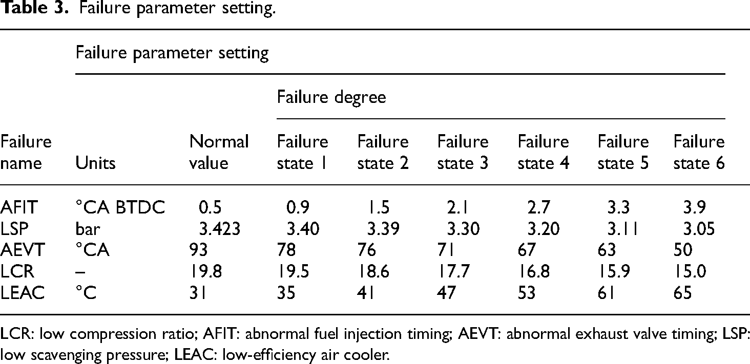
LCR: low compression ratio; AFIT: abnormal fuel injection timing; AEVT: abnormal exhaust valve timing; LSP: low scavenging pressure; LEAC: low-efficiency air cooler.

The single and multiple faults are all simulated by adjusting parameters in the engine simulation model. For example, the fault of intercooler efficiency drops (intercooler fouling or clogging) is captured by adjusting the heat transfer coefficient of the air cooler in the simulation model. Then the selected seven characteristic parameters are collected and compared with the normal values (NCs). In order to facilitate the comparison of abnormal values with NC when faults occur, the deviation rate (DR), which can be calculated by equation (1), is used to reflect the degree of abnormal values deviation from NC. The DR of the selected characteristic parameters is shown in Figure 7.

D R = \frac{X_{f} - X_{N C}}{X_{N C}} \times 100 %

(1)

where X_f represents the value of the selected characteristic parameter under fault conditions and X_NC represents the value under normal conditions.

Figure 7.

Deviation rate of the selected characteristic parameters.

Creation of fault data set

There are eight types of faults in total and 17 samples are set for each type of fault. Therefore, the total number of samples is 136 in this study, of which 90 are used for training purposes, 23 are used for validation purposes and the last 23 are used for testing purposes. The influence of different faults on characteristic parameters is shown in Table 4, and the coding information of different faults is shown in Table 5, which is used to recognize the fault type.

Table 4.

Diesel engine fault data set.

Fault	P_max (bar)	D_max (°CA)	IMEP (bar)	TT_exh.in (K)	TT_exh.out (K)	Fuel_inj (mg)	P_B20 (bar)
NC	172.96	12.74	19.22	612.6	470.74	12844.11	60.57
LCR	165.65	13.15	19.09	612.9	470.84	12852.89	58.79
AFIT	181.81	11.96	19.38	612.8	471.18	12844.12	60.19
LEAC	174.18	12.58	19.23	618.4	472.65	12939.15	62.23
AEVT	121.99	13.03	18.01	612.4	470.77	12917.83	36.09
LSP	159.65	12.80	19.23	657.9	513.74	13136.44	55.98
LSP and LCR	163.53	12.83	19.18	635.5	492.43	12,994.72	57.49
AEVT and LEAC	169.69	12.61	19.23	622.5	472.20	13039.50	60.14
LSP and AEVT	165.16	12.85	19.18	627.4	484.75	12943.57	57.02

NC: normal condition; LCR: low compression ratio; AFIT: abnormal fuel injection timing; AEVT: abnormal exhaust valve timing; LSP: low scavenging pressure; LEAC: low-efficiency air cooler; IMEP: indicated mean effective pressure.

Table 5.

Coding information of diesel engine failure.

Fault	AEVT	LEAC	AFIT	LCR	LSP
LCR	0	0	0	1	0
AFIT	0	0	1	0	0
LEAC	0	1	0	0	0
AEVT	1	0	0	0	0
LSP	0	0	0	0	1
LSP and LCR	0	0	0	1	1
AEVT and LEAC	1	1	0	0	0
LSP and AEVT	1	0	0	0	1

LCR: low compression ratio; AFIT: abnormal fuel injection timing; AEVT: abnormal exhaust valve timing; LSP: low scavenging pressure; LEAC: low-efficiency air cooler.

It can be seen from Table 4 that the values of different characteristic parameters are very different. It is necessary to normalize the characteristic parameters for easy comparison. The method of normalization can eliminate the influence of different value range on the accuracy of neural network. The method of normalization is shown in equation (2). The normalized characteristic parameters are shown in Table 6.

X = \frac{x - x_{m i n}}{x_{m a x} - x_{m i n}}

(2)

Table 6.

Normalization of characteristic parameters.

Fault	P_max (bar)	D_max (°CA)	IMEP (bar)	TT_exh.in (K)	TT_exh.out (K)	Fuel_inj (mg)	P_{B 2 0} (bar)
NC	0.8521	0.6555	0.8832	0.0044	0.0000	0.0000	0.9365
LCR	0.7299	1.0000	0.7883	0.0110	0.0023	0.0300	0.8684
AFIT	1.0000	0.0000	1.0000	0.0088	0.0102	0.0001	0.9220
LEAC	0.8725	0.5210	0.8905	0.1319	0.0444	0.3251	1.0000
AEVT	0.0000	0.8992	0.0000	0.0000	0.0001	0.2522	0.0000
LSP	0.6296	0.7059	0.8905	1.0000	1.0000	1.0000	0.7609
LSP and LCR	0.6944	0.7311	0.8540	0.5077	0.5044	0.5152	0.8187
AEVT and LEAC	0.7355	0.7059	0.8321	0.1033	0.1163	0.0555	0.7904
LSP and AEVT	0.7217	0.7479	0.8540	0.3297	0.3258	0.3402	0.8007

Creation of neural network model

The structure of the BP neural network

The fault database contains seven different characteristic parameters and relative fault coding information. Therefore, the input layer of the neural network is set to contain seven neurons, and the output layer of the neural network consists of five neurons. The number of hidden layer neurons is set as 5, 10 and 15 to compare the predictive performance. After experimental verification, the hidden layer containing 10 neurons can achieve the best results. The basic structure of the BP neural network is shown in Figure 8.

Figure 8.

Bayesian regularized (BP) neural network structure diagram.

BP neural network forward process

The transfer process of the BP neural network from the input layer to the hidden layer is shown in Figure 8. The data transfer process can be expressed by equation (3).

y_{j} = f (\sum_{i} w_{j i} x_{i} - θ_{j}) = f (n e t_{j}), n e t_{j} = \sum_{i} w_{j i} x_{i} - θ_{j}

(3)

where w_ji is the network updating weight between the input and hidden layer, x_i is the input parameter, which represents the fault characteristic parameter, and θ_j is the input layer threshold. The transfer process from the hidden layer to the output layer is also shown in Figure 8, the formulas are shown in equations (4) and (5).

n e t_{l} = \sum_{j} v_{l j} y_{j} - θ_{l}

(4)

\begin{aligned} E = & \frac{1}{2} \sum_{l} {(t_{l} - z_{l})}^{2} = \frac{1}{2} \sum_{l} {(t_{l} - f (\sum_{j} v_{l j} y_{j} - θ_{l}))}^{2} \\ = & \frac{1}{2} \sum_{l} {(t_{l} - f (\sum_{j} v_{l j} f (\sum_{i} w_{j i} x_{i} - θ_{j}) - θ_{l}))}^{2} \end{aligned}

(5)

where Z_l is the network output value, v_lj is the network weight between the hidden and output layer, y_j is the hidden layer output value, θ_l is the hidden layer threshold, t_l is the expected value, and E is the mean square error.

BP neural network weight updating process

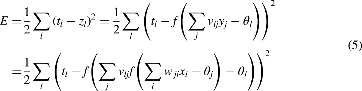
The derivation process of the output layer neuron by error function is shown in equations (6) to (9).

\frac{\partial E}{\partial v_{l j}} = \sum_{k = 1}^{n} \frac{\partial E}{\partial z_{k}} \cdot \frac{\partial z_{k}}{\partial v_{l j}} = \frac{\partial E}{\partial z_{l}} \cdot \frac{\partial z_{l}}{\partial v_{l j}}

(6)

\frac{\partial E}{\partial z_{l}} = \frac{1}{2} \sum_{k} [- 2 (t_{k} - z_{k}) \cdot \frac{\partial z_{k}}{\partial z_{l}}] = - (t_{l} - z_{l})

(7)

\frac{\partial z_{l}}{\partial v_{l j}} = \frac{\partial z_{l}}{\partial n e t_{l}} \cdot \frac{\partial n e t_{l}}{\partial v_{l j}} = f^{'} (n e t_{l}) \cdot y_{j}

(8)

\frac{\partial E}{\partial v_{l j}} = - (t_{l} - z_{l}) \cdot f^{'} (n e t_{l}) \cdot y_{j}

(9)

The derivation of hidden layer neurons by error function is shown in equations (10) to (16).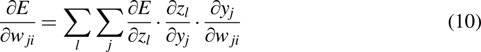

\frac{\partial E}{\partial w_{j i}} = \sum_{l} \sum_{j} \frac{\partial E}{\partial z_{l}} \cdot \frac{\partial z_{l}}{\partial y_{j}} \cdot \frac{\partial y_{j}}{\partial w_{j i}}

(10)

\frac{\partial E}{\partial z_{l}} = \frac{1}{2} \sum_{k} [- 2 (t_{k} - z_{k}) \cdot \frac{\partial z_{k}}{\partial z_{l}}] = - (t_{l} - z_{l})

(11)

\frac{\partial z_{l}}{\partial y_{j}} = \frac{\partial z_{l}}{\partial n e t_{l}} \cdot \frac{\partial n e t_{l}}{\partial y_{j}} = f^{'} (n e t_{l}) \cdot \frac{\partial n e t_{l}}{\partial y_{j}} = f^{'} (n e t_{l}) \cdot v_{l j}

(12)

\frac{\partial y_{j}}{\partial w_{j i}} = \frac{\partial y_{j}}{\partial n e t_{j}} \cdot \frac{\partial n e t_{j}}{\partial w_{j i}} = f^{'} (n e t_{j}) \cdot x_{i}

(13)

\begin{aligned} \frac{\partial E}{\partial w_{j i}} = & - \sum_{l} (t_{l} - z_{l}) \cdot f^{'} (n e t_{l}) \cdot v_{l j} \cdot f^{'} (n e t_{j}) \cdot x_{i} \\ = & - \sum_{l} δ_{l} v_{l j} f^{'} (n e t_{j}) \cdot x_{i} \end{aligned}

(14)

δ_{j}^{'} = f^{'} (n e t_{j}) \cdot \sum_{l} δ_{l} v_{l j}

(15)

\frac{\partial E}{\partial w_{j i}} = - δ_{j}^{'} x_{i}

(16)

where

x_{i}

is the input value, which represents the fault characteristic parameter, and

n e t_{j}

is the input value of the hidden layer neuron.

BP neural network weight gradient is shown in equations (17) to (20).

Δ v_{l j} = - η \frac{\partial E}{\partial v_{l j}} = - η δ_{l} y_{j}

(17)

v_{l j} (k + 1) = v_{l j} (k) + Δ v_{l j} = v_{l j} (k) + η δ_{l} y_{j}

(18)

Δ w_{j i} = - η^{'} \frac{\partial E}{\partial w_{j i}} = η^{'} δ_{j}^{'} x_{i}

(19)

w_{j i} (k + 1) = w_{j i} (k) + Δ w_{j i} = w_{j i} (k) + η^{'} δ_{j}^{'} x_{i}

(20)

where

η

is a constant learning rate. The update process of the neural network threshold is similar to the above process.

BP neural network proposed by Rumelhart and McClelland in 1986 is a useful tool for solving nonlinear problems.²⁶ Although it has a good performance in the field of fault diagnosis, it has some shortcomings in practice. The BP neural network uses the gradient descent method to gradually iterate the network weights and thresholds.²⁷ The gradient descent method will lead to a very large number of iterations under different gradient conditions due to the constant learning rate. In addition, the BP neural network usually falls into a local minimum, which makes it unable to solve optimization problems well.²⁸ In order to promote the diagnosis accuracy of multiple faults, the LM algorithm and BR algorithm are selected to optimize the BP neural network.

Levenberg Marquardt algorithm

The LM which combines the gradient descent method and the Gauss-Newton method is an optimization algorithm. Since the second derivative information is considered in the LM algorithm, the running speed of the network can be improved.

The optimization objective function is shown in equation (21).

‖ f (x + Δ x) ‖_{2}^{2}

(21)

The Taylor expansion of the objective function at x is shown in equations (22) and (23).

\begin{aligned} x : ‖ f (x + Δ x) = E (x) ‖_{2}^{2} \\ \approx ‖ f (x)_{2}^{2} ‖ + J (x) Δ x + \frac{1}{2} Δ x^{T} H Δ x \end{aligned}

(22)

E (x) = \sum_{i = 1}^{N} e_{i}^{2} (x)

(23)

where N represents the number of samples, E(x) is the error function,

e_{i}

is an error and H is the Hessian matrix which includes the matrix of the second derivative of the error function.

In Newton's algorithm, the Hessian matrix contains a matrix of the second derivative. In fact, the calculation process of the Hessian matrix is very complicated. The iteration step of the LM algorithm is shown in equations (24) and (25).

Δ x = - ({(J^{T} J + u I)}^{- 1} J^{T} f (x)), u \geq 0

(24)

H = J^{T} J

(25)

where I is the identity matrix and u is a non-negative number. The Hessian matrix is converted to the Jacobian matrix. J is the Jacobian matrix, which will greatly reduce the complexity of the calculation. If the value of u is large, the uI accounts for the main part. If the value of u is small, H occupies the main part. So the parameter u not only affects the direction of iteration, but also affects the size of iteration step, optimizing the shortcomings in the gradient descent method.

Bayesian regularization algorithm

The BR optimization algorithm can greatly improve the generalization ability of neural networks. The basic principle of the BR optimization algorithm is shown in equations (26) and (27).

E = \sum_{i = 1}^{n} {(t_{i} - a_{i})}^{2}

(26)

F = β E + α E_{w}, E_{w} = \frac{1}{M} \sum_{i = 1}^{M} w_{i}^{2}

(27)

where n is the number of samples, in this study n represents the fault category, t_i is the expected output value, a_i is the actual output of the network, and E is the mean square error. E_w is the sum of squared weights, w_i is the weight, α and β are the regularization parameters and F is the performance function.

The size of α and β determines the training goal of the network. The BR algorithm can automatically adjust the size of α and β during the network training process and obtain the optimal size of α and β.

Probabilistic neural network

The PNN was proposed by Dr DF Specht in 1989 and is mainly used in the research of classification problems. The PNN is composed of the input layer, the model layer, the summation layer and the output layer. The basic structure of PNN is shown in Figure 9. The input layer is the first layer and its function is to receive the input vector and pass it to the pattern layer. In this study, the input layer consists of seven characteristic parameters. The pattern layer consists of a training sample. The output probability of different neurons in the pattern layer is shown in equation (28).

\begin{aligned} φ_{i j} (X) = \frac{1}{\partial^{p} * {(2 π)}^{\frac{p}{2}}} e^{[- \frac{{(X - X_{i j})}^{T} * (X - X_{i j})}{2 \times \partial^{2}}]}, (i = 1, 2, \dots, M; j = 1, 2, \dots, L_{i}) \end{aligned}

(28)

where p is the number of training samples, ∂ is the spread value, X_ij represents the samples, i and j represent the category and sample, respectively, and M represents the number of categories. The number of neurons in the summation layer is equal to the fault categories. The probability density function of different fault categories is shown in equation (29).

f_{i} = \frac{\sum_{j = 1}^{L_{i}} φ_{i j} (X)}{L_{i}}

(29)

According to the probability estimation of the input vector, the output layer uses Bayesian classification rules to select the fault category with the maximum prior probability as the output. According to the Bayes minimum risk criterion, the method of classification is shown in equations (30) and (31).

If H_{i} L_{i} f_{i} (X) > H_{j} L_{j} f_{j} (X), then X \in M_{i}

(30)

If H_{i} L_{i} f_{i} (X) < H_{j} L_{j} f_{j} (X), then X \in M_{j}

(31)

where H_i and H_j are the prior probabilities of M_i and M_j, f_i and f_j are probability density functions of M_i and M_j, l_i and l_j are the cost factors. In practical applications, the spread value should be gradually adjusted to make the prediction best. According to the experimental results, the spread value is set as 2.5 in this study.

Diagnostic performance and comparative analysis

In this study, a test set containing 23 samples was set up to test the accuracy of the established networks. Among them, nine samples of multiple faults were specially arranged to test the effect of the three neural networks on multiple fault diagnosis. The order of the 23 samples and the normalized results of the seven characteristic parameters are shown in Table 7. The running speed of the neural network can be calculated using equation (32). Equation (33) is used to calculate the diagnostic accuracy rate of the neural networks. The relative coding information of the testing set which is used to identify faults is shown in Table 8.

S p e e d = C P U_{s t a r t} - C P U_{e n d}

(32)

A c c u r a c y = \frac{C N - F N}{N}

(33)

where N represents the total number of testing sets, d_i represents the expected output, and y_i represents the actual output of the neural network. CPU_start and CPU_end represent the time when the neural network calculation starts and ends, respectively. CN and FN represent the number of correctly predicted samples and the number of wrongly predicted samples, respectively.

Figure 9.

The structure of the probabilistic neural network.

Table 7.

Normalization of fault samples.

Fault	P_max	D_max	IMEP	TT_exh.in	TT_exh.out	Fuel_inj	P_B20
1. LSP and LCR	0.5010	0.7043	0.6789	0.2010	0.1948	0.2586	0.7513
2. AFIT	0.8769	0.2045	0.9270	0.0038	0.0043	0.0203	0.8769
3. LEAC and AEVT	0.5629	0.6431	0.7235	0.1371	0.0501	0.4378	0.8431
4. LSP	0.3218	0.7031	0.7215	1.0000	1.0000	1.0000	0.5458
5. LCR	0.5389	0.7343	0.6561	0.0145	0.0053	0.0861	0.8122
6. LEAC and AEVT	0.5470	0.6561	0.7258	0.2232	0.0903	0.6470	0.8375
7. LEAC	0.6424	0.6361	0.7252	0.1916	0.0807	0.4491	1.0000
8. LCR	0.4744	0.8047	0.5835	0.0142	0.0041	0.0924	0.7663
9. AFIT	1.0000	0.0000	1.0000	0.0000	0.0039	0.0000	0.8685
10. AEVT and LSP	0.5074	0.6826	0.6663	0.1022	0.0953	0.1678	0.7351
11. LSP and LCR	0.4304	0.7293	0.6271	0.254	0.2473	0.3213	0.7134
12. AFIT	0.8525	0.2275	0.9101	0.0034	0.0033	0.0222	0.8405
13. AEVT and LSP	0.4005	0.6994	0.6145	0.2429	0.2521	0.2614	0.5693
14. AEVT	0.0000	0.7235	0.0000	0.0049	0.0037	0.1671	0.0000
15. LCR	0.1718	1.0000	0.2196	0.0222	0.0047	0.1521	0.5236
16. LCR	0.3071	0.9167	0.3935	0.0180	0.0043	0.1199	0.6433
17. LSP and LCR	0.5802	0.7025	0.7070	0.0564	0.0491	0.1175	0.8388
18. AFIT	0.9509	0.0922	0.9724	0.0015	0.0041	0.0076	0.8718
19. LSP	0.4771	0.6886	0.7224	0.4143	0.4115	0.4528	0.6989
20. LEAC and AEVT	0.5568	0.6702	0.7241	0.0841	0.0245	0.3351	0.8139
21. LCR	0.2735	0.9181	0.3519	0.0190	0.0043	0.1282	0.6177
22. LCR	0.2058	0.9726	0.2652	0.0213	0.0046	0.1437	0.5651
23. LEAC and AEVT	0.5951	0.6688	0.7237	0.0253	0.0000	0.1568	0.8537

Table 8.

Coding information of the testing set.

Fault number	1	2	3	4	5	6	7	8	9	10	11	12	13	14	15	16	17	18	19	20	21	22	23
LEAC	0	0	1	0	0	1	1	0	0	0	0	0	0	0	0	0	0	0	0	1	0	0	1
AEVT	0	0	1	0	0	1	0	0	0	1	0	0	1	1	0	0	0	0	0	1	0	0	1
LSP	1	0	0	1	0	0	0	0	0	1	1	0	1	0	0	0	1	0	1	0	0	0	0
AFIT	0	1	0	0	0	0	0	0	1	0	0	1	0	0	0	0	0	1	0	0	0	0	0
LCR	1	0	0	0	1	0	0	1	0	0	1	0	0	0	1	1	1	0	0	0	1	1	0

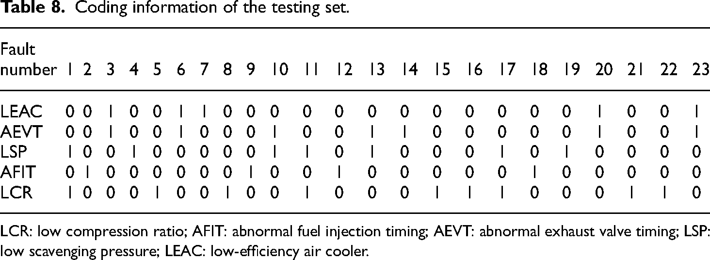
LCR: low compression ratio; AFIT: abnormal fuel injection timing; AEVT: abnormal exhaust valve timing; LSP: low scavenging pressure; LEAC: low-efficiency air cooler.

The predicted values of the LM-BP neural network on the testing set are shown in Table 9. It can be seen that among the prediction results of the total 23 samples, 22 are correct, but sample number 17 is false, which is blacked out in the table. The accuracy of this network for the total testing set is 95.65%. The diagnosis time of LM-BP for all 23 samples is 0.78 s. From the perspective of fault types, the LM-BP neural network correctly diagnoses all the single faults, while for the nine multiple faults, only sample number 17 gets the wrong result. The diagnostic accuracy rate of the LM-BP neural network for single faults is 100%, and for multiple faults is 88.89%.

Table 9.

LM-BP neural network output value.

Fault number	1	2	3	4	5	6	7	8	9	10	11	12	13	14	15	16	17	18	19	20	21	22	23
LEAC	0	0	1	0	0	1	1	0	0	0	0	0	0	0	0	0	0	0	0	1	0	0	1
AEVT	0	0	1	0	0	1	0	0	0	1	0	0	1	1	0	0	0	0	0	1	0	0	1
LSP	1	0	0	1	0	0	0	0	0	1	1	0	1	0	0	0	1	0	1	0	0	0	0
AFIT	0	1	0	0	0	0	0	0	1	0	0	1	0	0	0	0	0	1	0	0	0	0	0
LCR	1	0	0	0	1	0	0	1	0	0	1	0	0	0	1	1	0	0	0	0	1	1	0

LM-BP: Levenberg Marquardt back propagation; LCR: low compression ratio; AFIT: abnormal fuel injection timing; AEVT: abnormal exhaust valve timing; LSP: low scavenging pressure; LEAC: low-efficiency air cooler.

The predicted values of the BR-BP neural network on the testing set are shown in Table 10. The total correct number is 19, and the sample numbers 1, 10, 11 and 17 are false. The accuracy of this network for the entire testing set is 82.61%. The total time-consuming is 3.17 s. Comparing the sample number with Table 7, it can be seen that all the samples with incorrect diagnoses are multiple faults. The BR-BP neural network also gets 100% accuracy for a single fault, but for multiple faults, the diagnostic accuracy rate is only 55.56%.

Table 10.

BR-BP neural network output value.

Fault number	1	2	3	4	5	6	7	8	9	10	11	12	13	14	15	16	17	18	19	20	21	22	23
LEAC	0	0	1	0	0	1	1	0	0	0	0	0	0	0	0	0	0	0	0	1	0	0	1
AEVT	0	0	1	0	0	1	0	0	0	2	1	0	1	1	0	0	1	0	0	1	0	0	1
LSP	1	0	0	1	0	0	0	0	0	1	1	0	1	0	0	0	1	0	1	0	0	0	0
AFIT	0	1	0	0	0	0	0	0	1	0	0	1	0	0	0	0	0	1	0	0	0	0	0
LCR	0	0	0	0	1	0	0	1	0	0	1	0	0	0	1	1	1	0	0	0	1	1	0

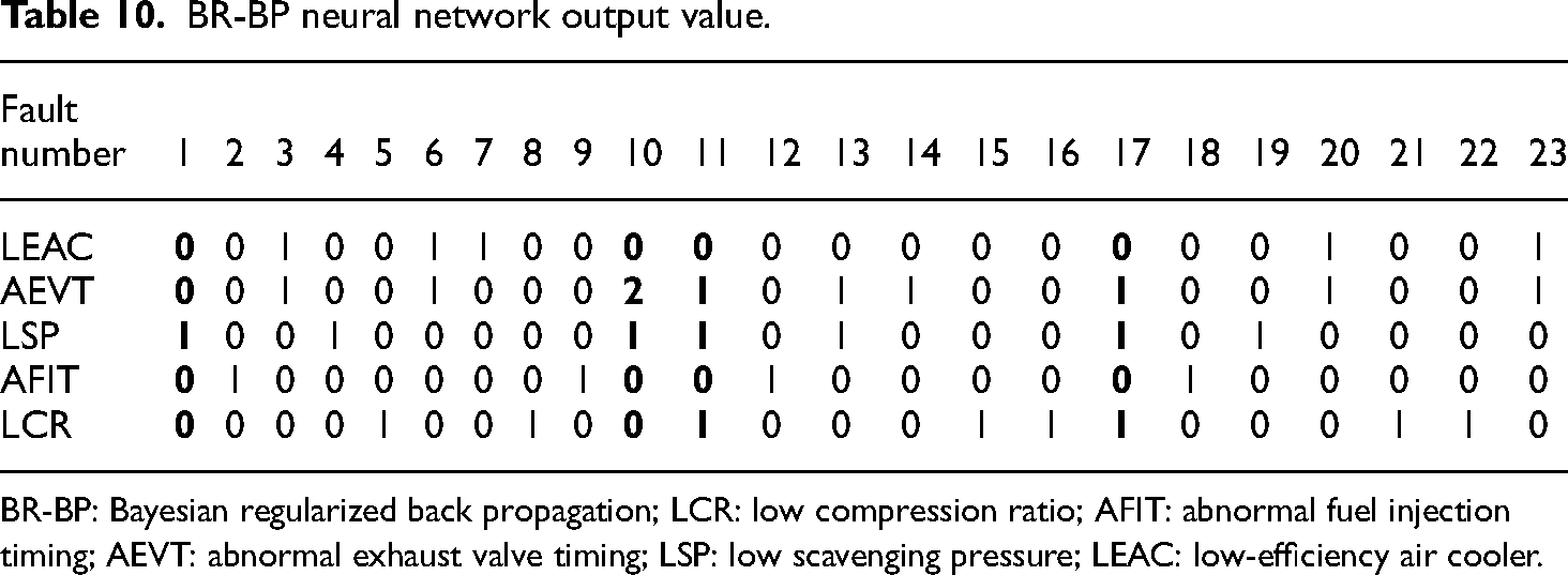
BR-BP: Bayesian regularized back propagation; LCR: low compression ratio; AFIT: abnormal fuel injection timing; AEVT: abnormal exhaust valve timing; LSP: low scavenging pressure; LEAC: low-efficiency air cooler.

In order to facilitate the PNN to identify the faults, all eight types of faults are coded from one to eight before starting the diagnosis, as shown in Table 11. The predicted values for the testing set of PNN are shown in Table 12. There are six wrong diagnosis results, which are numbered 1, 3, 7, 17, 19 and 23. Among them, samples 7 and 19 are single faults, and the remaining four faults are multiple faults. Obviously, PNN has not achieved a completely correct diagnosis for the single fault, with an accuracy rate of only 85.71%, and the accuracy rate for the multiple fault is even lower, only 55.56%. The diagnostic accuracy rate of PNN for the entire testing set is 73.91%, and the total time-consuming is 0.24 s.

Table 11.

Fault coding for PNN.

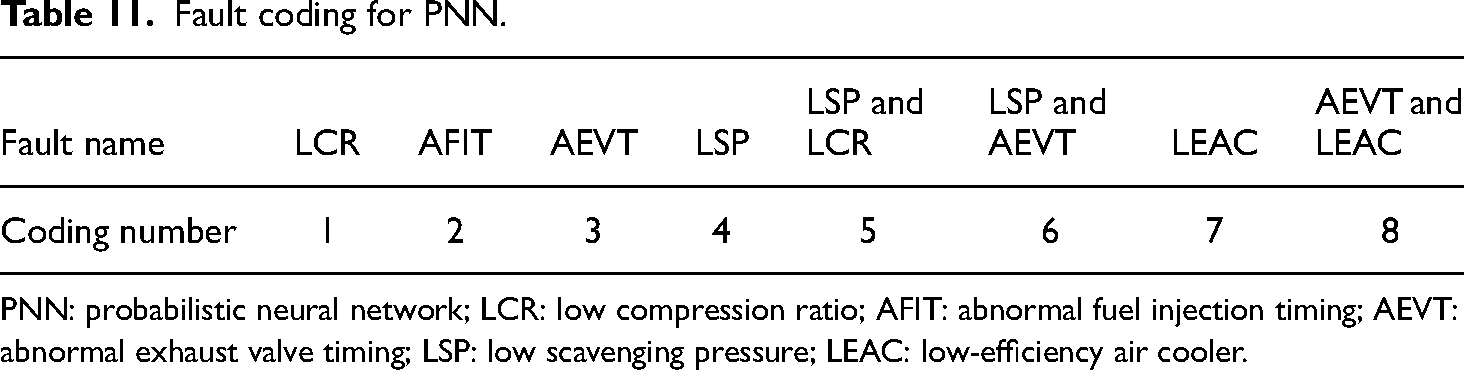
Fault name	LCR	AFIT	AEVT	LSP	LSP and LCR	LSP and AEVT	LEAC	AEVT and LEAC
Coding number	1	2	3	4	5	6	7	8

PNN: probabilistic neural network; LCR: low compression ratio; AFIT: abnormal fuel injection timing; AEVT: abnormal exhaust valve timing; LSP: low scavenging pressure; LEAC: low-efficiency air cooler.

Table 12.

Probabilistic neural network (PNN) output value.

Fault number	1	2	3	4	5	6	7	8	9	10	11	12	13	14	15	16	17	18	19	20	21	22	23
Expected value	5	2	8	4	1	8	7	1	2	6	5	2	6	3	1	1	5	2	4	8	1	1	8
Predicted values	3	2	3	4	1	8	8	1	2	6	5	2	6	3	1	1	1	2	2	8	1	1	3
True or false	F	T	F	T	T	T	F	T	T	T	T	T	T	T	T	T	F	T	F	T	T	T	F

The diagnostic performance of the established three networks on the test set is summarized in Table 13. It can be found that both LM-BR and BR-BP neural networks can achieve a 100% diagnostic accuracy rate for a single fault, and the less effective PNN also gives a diagnostic accuracy rate of 85.71%. However, for multiple faults, none of the three neural networks can achieve a 100% diagnostic accuracy rate, the highest diagnostic accuracy rate is 88.89%, obtained by the LM-BR neural network. It verifies the difficulty of accurate diagnosis of the multiple faults again. Comparing the diagnosis results of the three neural networks, it can be found that the LM-BR neural network can give a relatively satisfactory diagnostic accuracy rate for both single faults and multiple faults, and the diagnosis time is also relatively short. The BR-BP neural network can correctly diagnose single faults, but its diagnostic effect on multiple faults is not satisfactory, and the diagnosis time is the longest. Although PNN has the fastest diagnosis speed, its diagnostic accuracy rate is the worst among the established three neural networks, whether it is for single faults or multiple faults.

Table 13.

Performance of the neural networks.

Neural network name	For all the fault		For single fault	For multiple faults
Neural network name	Accuracy	Speed	Accuracy	Accuracy
LM-BP	95.65%	0.78	100%	88.89%
BR-BP	82.61%	3.17	100%	55.56%
PNN	73.91%	0.24	85.71%	55.56%

LM-BP: Levenberg Marquardt back propagation; BR-BP: Bayesian regularized back propagation; PNN: probabilistic neural network.

Conclusion

The principles of LM-BP, BR-BP neural networks and PNN are briefly introduced and the diagnosis methods based on these neural networks are established in this study. The established diagnosis methods are used to diagnose the multiple faults in an ocean-going marine diesel engine. The diagnostic performances are compared and the following conclusions can be drawn:

For the single faults of the ocean-going marine diesel engines, a very high diagnostic accuracy rate can be achieved. Among the three methods established in this study, both the diagnosis methods based on the LM-BR and BR-BP neural networks have achieved 100% accuracy.

For the multiple faults of the ocean-going marine diesel engines, it is still very difficult to diagnose. The highest diagnostic accuracy of the three methods established in this study is only 88.89%. Diagnosis methods for multiple faults still need continuous improvement, which will promote the development of smart ships.

Among the three methods established in this study, the diagnosis method based on the LM-BR neural network has a more ideal effect than the diagnosis methods based on the BR-BP neural network and PNN.

Footnotes

Acknowledgements

The authors would like to acknowledge the financial support from the Navy University of Engineering and the National Natural Science Foundation of China (no. 51909154), the Shanghai High-level Local University Innovation Team (Maritime Safety & Technical Support), and Shanghai Engineering Research Center of Ship Intelligent Maintenance and Energy Efficiency (no. 20DZ2252300).

Declaration of conflicting interests

The author(s) declared no potential conflicts of interest with respect to the research, authorship, and/or publication of this article.

Funding

The author(s) disclosed receipt of the following financial support for the research, authorship, and/or publication of this article: This work was supported by the National Natural Science Foundation of China, Shanghai Engineering Research Center of Ship Intelligent Maintenance and Energy Efficiency, Shanghai High-level Local University Innovation Team (Maritime Safety & Technical Support) (grant numbers 51909154, 20DZ2252300).

ORCID iD

Lijiang Wei

Author biographies

Guoqing Zhu is currently a Research Associate in Research Institute of Equipment Simulation Technology, Naval University of Engineering, China. His research interests focus on design, simulation and optimization of power machinery and thermal systems.

Lin Huang was born in Jiangxi province, China in 1992. He received the B.S. degree and M.S. degree in Ocean Engineering from the Army Military Transportation University of China in 2012 and 2014 respectively and the Ph.D. degree of Power engineering from Naval University of Engineering, China, 2018. He is currently working as a lecturer at Naval University of Engineering, China. His research interests include prognostics and system health management, development of data-driven-based algorithms for multivariate time series for improving the efficiency of critical industrial machines.

Jiapeng Yin received his master's degree from the Merchant Marine College of Shanghai Maritime University and is now an engineer at Alfa Laval Technology Company, Shanghai, China. His research interests focus on marine diesel engine fault analysis and diagnosis.

Wen Gai received her master's degree from the College of information engineering of Shanghai Maritime University. Her research interests focus on the application of intelligent algorithms in marine diesel engines.

Lijiang Wei is currently an Associate Professor in Merchant Marine College, Shanghai Maritime University, China. His research interests focus on the in-cylinder combustion process and fault diagnosis of marine diesel engines.

Appendix

References

Wan

Yang

Sun

. A method for monitoring lubrication conditions of journal bearings in a diesel engine based on contact potential. Appl Sci 2020; 10: 5199.

Cheng

Qiao

Jin

, et al. A novel fault diagnosis method for diesel engine based on MVMD and band energy. Shock Vib 2020, 1–17. Article ID 8247194. https://doi.org/10.1155/2020/8247194

Knežević

Orović

Stazić

, et al. Fault tree analysis and failure diagnosis of marine diesel engine turbocharger system. J Mar Sci Eng 2020; 8: 1004.

Sala

Tormos

Macian

. A fuzzy diagnosis module for oil analysis in industrial diesel engines. IFAC Proc Vol 2004; 37: 199–204.

Puchalski

. A technique for the vibration signal analysis in vehicle diagnostics. Mech Syst Signal Process 2015; 56–57: 173–180.

Taghizadeh

Mandavian

. Fault detection of injectors in diesel engines using vibration time–frequency analysis. Appl Acoust 2019; 143: 48–58.

Yao

Song

, et al. Intelligent fault diagnosis method of common rail injector based on composite hierarchical dispersion entropy and improved least squares support vector machine. Digit Signal Process 2021; 114: 103054.

Tse

Yang

, et al. EMD-based fault diagnosis for abnormal clearance between contacting components in a diesel engine. Mech Syst Signal Process 2010; 24: 193–210.

Antonić

Vukić

Kuljača

. Marine diesel engine faults diagnosis based on observed symptoms and expert knowledge. IFAC Proc Vol 2003; 36: 133–138.

10.

Yin

Chen

Guan

, et al. Research on fault identification method of diesel engine based on PCA-PNN. J Wuhan Univ Technol Transp Sci Eng 2021; 45: 270–275.

11.

Wang

Chen

Guan

, et al. Research on the fault monitoring method of marine diesel engines based on the manifold learning and isolation forest. Appl Ocean Res 2021; 112: 102681.

12.

Huang

Xie

Huang

. Research on thermal fault diagnosis of marine diesel engine based on SPA. Ship Eng 2014; 36: 48–51.

13.

Zhao

, et al. Machine learning-based wear fault diagnosis for marine diesel engine by fusing multiple data-driven models. Knowl Based Syst 2020; 190: 105324.

14.

Jafarian

Mobin

Jafari

, et al. Misfire and valve clearance faults detection in the combustion engines based on a multi-sensor vibration signal monitoring. Measurement (Mahwah NJ) 2018; 128: 527–536.

15.

Nahim

Younes

Shraim

, et al. Modeling with fault integration of the cooling and the lubricating systems in marine diesel engine: experimental validation. IFAC-Papers Online 2016; 49: 570–575.

16.

Cao

Xie

, et al. Diesel engine fault diagnosis method based on multi-source information fusion. Marine Technology 2020: 73–80. +92.

17.

Zhang

Liu

. Charging stations expansion planning under government policy driven based on Bayesian regularization backpropagation learning. Neurocomputing 2020; 416: 47–58.

18.

Nawi

Khan

Rehman

. A new Levenberg Marquardt based back propagation algorithm trained with cuckoo search. Proc Technol 2013; 11: 18–23.

19.

Castresana

Gabina

Martin

, et al. Comparative performance and emissions assessments of a single-cylinder diesel engine using artificial neural network and thermodynamic simulation. Appl Therm Eng 2021; 185: 116343.

20.

Rubio

JAP

Vera-García

Grau

, et al. Marine diesel engine failure simulator based on thermodynamic model. Appl Therm Eng 2018; 144: 982–995.

21.

Hariram

Vagesh Shangar

. Influence of compression ratio on combustion and performance characteristics of direct injection compression ignition engine. Alexandria Eng J 2015; 54: 807–814.

22.

Wei

Yao

Han

, et al. Effects of methanol to diesel ratio and diesel injection timing on combustion, performance and emissions of a methanol port premixed diesel engine. Energy 2016; 95: 223–232.

23.

Nora

Lanzanova

TDM

Zhao

. Effects of valve timing, valve lift and exhaust backpressure on performance and gas exchanging of a two-stroke GDI engine with overhead valves. Energy Convers Manage 2016; 123: 71–83.

24.

Jayashankara

Ganesan

. Effect of fuel injection timing and intake pressure on the performance of a DI diesel engine – a parametric study using CFD. Energy Convers Manage 2010; 51: 1835–1848.

25.

Wei

Liu

, et al. Nitrogen oxides reduction effect and the influence mechanism of exhaust valve lift on a two-stroke marine diesel engine. J Eng Gas Turb Power Trans ASME 2019; 141: 081006.

26.

Liu

Wen

Wang

, et al. Research on fault diagnosis method of board-level circuit based on genetic algorithm. Procedia Comput Sci 2018; 131: 495–501.

27.

Duddu

Pulugurtha

Mane

, et al. Back-propagation neural network model to predict visibility at a road link-level. Transp Res Interdiscip Perspect 2020; 8: 100250.

28.

Han

Hong

Meng

, et al. Temperature drift modeling and compensation of capacitive accelerometer based on AGA-BP neural network. Measurement (Mahwah NJ) 2020; 164: 108019.

Multiple faults diagnosis for ocean-going marine diesel engines based on different neural network algorithms

Abstract

Keywords

Introduction

Selection of diesel engine failure

Basic parameters of the marine diesel engine

Characteristic parameters

Fault simulation

Creation of fault data set

Creation of neural network model

The structure of the BP neural network

BP neural network forward process

BP neural network weight updating process

Levenberg Marquardt algorithm

Bayesian regularization algorithm

Probabilistic neural network

Diagnostic performance and comparative analysis

Conclusion

Footnotes

Acknowledgements

Declaration of conflicting interests

Funding

ORCID iD

Author biographies

Appendix

References