Sage Journals: Discover world-class research

Abstract

Balises are key safety-critical components in many railway systems. However, as the usage time of balises increases, the performance of the physical devices within a balise information transmitting module will gradually deteriorate. This deterioration leads to a decline in the output performance of a balise information transmitting circuit. It is crucial to identify the key physical devices that contribute to the degradation of the balise information transmitting circuit's output performance, as this can provide a foundation for assessing the health status and predicting the residual life of a balise. Consequently, this paper proposes a sensitivity analysis method for balise information transmitting module circuits that considers performance degradation and model uncertainty. First, a surrogate model for balise information transmitting circuits is established based on a deep neural network that integrates both physical knowledge and experimental data. Random sampling-high-dimensional model representation method is employed to analyse the sensitivity of the degraded input and scalar output of the balise information transmitting circuit surrogate model, thereby clarifying the key physical devices that impact performance degradation. Finally, the model uncertainty introduced by the establishment of the balise information transmitting circuit surrogate model is analysed. The experimental results indicate that the proposed method effectively identifies the key physical devices that influence the degradation of output performance in the balise information transmitting circuit.

Keywords

Balise performance degradation sensitivity analysis random sampling-high-dimensional model representation deep neural network uncertainty analysis

Introduction

In modern railway systems, a balise serves as a fundamental piece of equipment for correcting train positioning and transmitting safety control information to a train.¹ As the usage duration of a balise increases, the performance of each physical device within balise information transmitting (BIT) circuits gradually deteriorates, leading to a decline in the overall performance of BIT circuits. This degradation adversely affects the health status of balises, posing significant risks to the safe operation of trains. With the rapid advancement of information and automation technologies, intelligent operation and maintenance have emerged as crucial strategies for ensuring effective railway fault diagnosis and maintenance.² Condition-based maintenance and predictive maintenance are essential approaches for implementing intelligent operation and maintenance. By consistently monitoring the status of key system components, the real-time health status of a system can be assessed, and the remaining useful life of a system can be predicted, enabling maintenance to be performed based on the health status and the remaining useful life of a system.³ Identifying the key physical devices that contribute to the performance degradation of BIT circuits is vital, as it provides a foundation for assessing the health status and predicting the residual life of balises.

Currently, research on the performance degradation analysis of electronic equipment, such as a balise, is primarily conducted from two perspectives: the failure mechanisms at the circuit level and the degradation factors at the physical device level. Numerous studies have explored various failure mechanisms and their impacts on the performance of radio frequency (RF) circuits. For instance, Naseh et al.⁴ found that hot carrier injection leads to a decline in the current–voltage characteristics of oscillators, resulting in a slight alteration of the oscillation frequency. Saarinen and Frisk⁵ examined the influence of environmental pressure on the reliability of radio frequency identification (RFID) tags by varying combinations of temperature and humidity tests. In addition to classical failure physical models, some scholars employ accelerated ageing experiments, such as high temperature, electrical stress, and mechanical stress, to obtain experimental data and analyse the degradation process of electronic equipment or components based on a random process model or probability distribution function. To derive the physical failure model of a bipolar junction transistor (BJT) based on the Arrhenius model, the Gamma distribution was utilised to fit the high-temperature accelerated degradation data.⁶ Keimasi et al.⁷ applied a three-parameter Weibull distribution to model the effects of mechanical stress on the degradation of capacitors in printed circuit boards. That research primarily focused on the failure mechanisms at the circuit level. In terms of studying the causes of degradation at the physical device level, thermal stress, electrical stress,^8,9 and mechanical stress¹⁰ are the main factors contributing to the ageing failure of metallised film capacitors, multi-layer ceramic capacitors, and integrated capacitors. The degradation of BJTs is influenced by a combination of electrical stress, thermal stress, and radiation stress.^11,12

To identify the key physical devices that impact the degradation of BIT circuit output performance, it is crucial to analyse both the variability in BIT circuit output performance and the uncertainty related to the degradation of these physical devices using measures that account for uncertainty. In the field of reliability, sensitivity analysis serves as a key tool for the measurement of importance under uncertainty.^13,14 However, there are several challenges to be overcome to employ sensitivity analysis to assess the performance degradation of BIT circuits. These can be summarised as follows: (1) the model error or deviation between the BIT circuit simulation model and the actual balise circuit, which will compromise the accuracy of the sensitivity analysis results. (2) During performance degradation of a BIT circuit, the input and output of the circuit model are time-dependent dynamic functions, rendering classical (time invariant) sensitivity analysis methods based on the Sobol index inappropriate for the analysis. (3) A BIT circuit model exhibits characteristics of non-linearity, dynamic time correlation, and high computational demands, resulting in significant computational complexity when performing sensitivity analysis.

The usual modelling and analysis methods for a balise, as an RF circuit system, rely on circuit theory, which is considered the most reliable approach.^15,16 However, a traditional balise circuit model is often too time-consuming to be practical for sensitivity analysis, particularly when accounting for physical device degradation and time dependence. With the rise of artificial intelligence technology, machine learning methods, particularly deep neural networks (DNNs), have been widely adopted in the modelling of RF circuits and fault testing. Machine learning techniques can effectively model a system using extensive simulation data, making them suitable for sensitivity analysis. Consequently, machine learning-based modelling methods present a viable solution for addressing the sensitivity analysis challenge associated with complex circuits.

Given the complexity of dynamic systems characterised by non-linearity and internal interactions, a global sensitivity analysis (GSA) method is the preferred approach for analysing the sensitivity of BIT circuits.¹⁷ The global sensitivity index (GSI) is solved by GSA, and then the key physical devices can be determined. A variance-based sensitivity analysis method, known for its theoretical simplicity and ease of application, has emerged as the most widely utilised GSA method in both industry and academia.^18–21 Extensive literature exists on variance-based sensitivity analysis methods. For dynamic model systems, Campbell et al.²² expanded the time-dependent output function into a set of basis functions by selecting appropriate scalar functions and calculating sensitivity indices based on the statistics of the basis function coefficients. This scalar function expansion method was extended to multivariate outputs, leading to the proposal of a generalised sensitivity index that comprehensively characterises the influence of each parameter on the entire time-series output.²³ A dynamic system is transformed into a multi-input, multi-output problem through input time discretisation and scalar function output, and is analysed via multivariate variance decomposition. However, practical issues associated with multivariate outputs often result in significant computational demands when employing commonly used output decomposition methods.

To address the challenges associated with time-consuming sensitivity index solutions, a sensitivity solution method based on a meta-model is introduced. Serving as a model of models, the meta-model provides an accurate representation of complex systems and effectively describes the input–output relationship, allowing for the evaluation of how inputs impact outputs.²⁴ A sensitivity solution method using meta-models can significantly reduce computational complexity while maintaining calculation accuracy.

To address the above challenges, this paper proposes a sensitivity analysis method for BIT module circuits that considers performance degradation and model uncertainty. The primary contributions are as follows:

The dynamic system of BIT circuits is discretised and transformed into a multi-input, multi-output static system for sensitivity analysis. Appropriate sensitivity indices are selected to characterise the influence of BIT circuit's input parameters on its output.

Based on DNN models, a surrogate model for the BIT circuit is established that integrates physical knowledge data and experimental data, utilising the mechanism of pre-training with physical knowledge data and updating training with experimental data. The uncertainty introduced by the surrogate model is analysed, and the surrogate model can accurately characterise the performance degradation characteristics of the BIT circuit.

Using the degraded data input and scalar output from the BIT circuit surrogate model, a random sampling-high-dimensional model representation (RS-HDMR) method is employed to analyse the sensitivity of the model. Based on the calculated sensitivity index, the key physical devices that affect the performance degradation of the BIT circuit are identified. The RS-HDMR method demonstrates significant advantages in both computational accuracy and efficiency.

Preliminaries

Operating principle of BIT module

A balise is a specialised electronic device utilised in train control systems, operating on the principles of RFID technology.²⁵ It is categorised into two types: active balise and passive balise. Active balise continually transmits variable information from the lineside electronic unit to the train, while passive balise only transmits fixed information, that is stored locally when it is activated by a train. The balise information is crucial for the safe operation of the train control system, typically consisting of data bits, control bits, and check bits.²⁶ This information structure is designed to ensure the security and reliability of the message. The functionality of balises in sending messages is intrinsically linked to the performance of the BIT circuit. When a train passes by, the balise is activated, and its dynamic operational process is illustrated in Figure 1.

Figure 1.

Dynamic working process of the balise when the train passes.

As illustrated in Figure 1, the dynamic working process of a balise consists of four interconnected links: downlink energy transmission, balise energy reception, balise information transmission, and uplink information transmission. Among these, the processes of downlink energy transmission and uplink information transmission rely on electromagnetic induction, while the functions of balise energy reception and information transmission are achieved through distinct physical circuits. Using the circuit topology of the LC voltage-controlled oscillator, an equivalent simulation model of the BIT circuit has been constructed, as depicted in Figure 2.²⁷

Figure 2.

Equivalent simulation model of the balise information transmitting (BIT) circuit.

In Figure 2, the primary physical components of the BIT circuit include inductors (L₁, L₂), capacitors (C₁–C₉), resistors (R₁–R₃), BJTs (Q₁–Q₄), and low dropout (LDO) regulators (output V_dd, V_En). The BIT circuit employs an LC resonant circuit and a cross-coupling pair (Q₁, Q₂) to generate negative resistance, compensating for the resistive losses inherent in the LC resonant circuit. Within the LC resonant circuit, the 4.234 MHz transmitting antenna and matching circuit in the balise are effectively represented as inductors (L₁, L₂) and capacitors (C₈, C₉). The bias voltage V_dd serves as the power supply voltage, while the bias voltage V_En represents the enabling voltage for the cross-coupling circuit, which is provided by the balise energy-receiving circuit. The switch voltage functions as the control voltage for BJTs (Q₃, Q₄). These BJTs (Q₃, Q₄) can alter the number of capacitors in the LC resonant circuit, thereby adjusting the oscillation frequency to produce the frequency shift keying dual-frequency oscillation signal. The dual-frequency oscillation output frequency of the balise can be expressed by²⁸

f_{1, 2} = \frac{1}{2 π \sqrt{L_{T} (C_{on, off} + C_{par} + C_{couple})}}

(1)Where, f_1,2 represents the high-frequency signal and low-frequency signal generated by the balise frequency switching, L_T and C_par represent the inductance and capacitance values of the information transmitting antenna and the matching circuit in the LC resonant circuit, respectively. C_on and C_off represent the shunt capacitance of the cross-coupled circuit when BJTs (Q₃, Q₄) are turned on and off, respectively. C_couple is the capacitance of the cross-coupled circuit incorporated into the resonant circuit, then:

L_{T} = L_{1} + L_{2}

(2)

C_{par} = C_{8} / / C_{9}

(3)

C_{on} = C_{5} / / C_{6}

(4)

C_{off} = C_{5} / / C_{6} / / C_{7}

(5)

\begin{aligned} C_{couple} = C_{3} / / (C_{2} + C_{Q 2_bc} + C_{Q 2_be}) or \\ C_{couple} = C_{4} / / (C_{1} + C_{Q 1_bc} + C_{Q 1_be}) \end{aligned}

(6)where the operator ‘//’ represents the series calculation of capacitance. C_{Q1_bc}, C_{Q1_be}, C_{Q2_bc}, and C_{Q2_be} are the base-to-collector capacitance and the base-to-emitter capacitance of BJTs (Q₁, Q₂), respectively.²⁹

The output current of the BIT antenna can be obtained by the following equation:

I_{L_{1}} = \frac{V_{n} - V_{dd}}{2 π f_{1, 2} \cdot L_{1}} or I_{L_{2}} = \frac{V_{p} - V_{dd}}{2 π f_{1, 2} \cdot L_{2}}

(7)where V_n and V_p are the collector voltages of BJTs (Q₁, Q₂). The expression of the induced voltage of the balise uplink is

U (t) = A_{BIV} \cdot \frac{V_{dd} \cdot \sin (2 π f_{1, 2} \cdot t)}{2 π f_{1, 2} \cdot L_{1}}

(8)where A_BIV is the amplitude of the induced voltage signal.

In summary, the changes of the supply voltage V_dd and the oscillation frequency f_1,2 of the BIT circuit will affect the output current of the BIT antenna and the uplink-induced voltage. The V_dd is related to the output of the balise energy-receiving circuit.

Scalar output parameter extraction of BIT module

The classical sensitivity analysis method based on the Sobol index is inadequate for analysing systems with dynamically time-correlated outputs. Therefore, it is crucial to extract appropriate scalar parameters that can effectively characterise the dynamic time output curve characteristics of the BIT circuit. According to the European standard ‘ERTMS/ETCS Class 1, FFFIS for EuroBalise’ (SUBSET-036) and the analysis presented in the previous section, the ground balise transmitting antenna communicates uplink information to the train receiving antenna through electromagnetic induction, ultimately resulting in an induced voltage at the train receiving antenna. Measuring the output frequency and current of the BIT circuit is challenging, as they do not directly influence the train receiving antenna. Consequently, the balise uplink-induced voltage is utilised as the final output of the BIT circuit. However, a single scalar parameter is insufficient to comprehensively characterise the output performance of the balise. Therefore, key scalar features will be extracted to describe the uplink-induced voltage of the balise.

The ‘ERTMS/ETCS Class 1, FFFIS for EuroBalise’ (SUBSET-036) specifies six test parameters for assessing the characteristics of balise uplink signals: centre frequency, frequency deviation, signal bandwidth, amplitude jitter, mean data rate, and maximum time interval error. Notably, while the mean data rate is a fixed parameter, the other five parameters are variable scalars. Consequently, for the same output, these scalar values will vary depending on the selected test duration or test interval. Therefore, the existing test parameters cannot be directly utilised to characterise the output of the balise, necessitating appropriate conversions.

The centre frequency, frequency deviation, and signal bandwidth can be determined by mapping the induced voltage of the balise uplink using the fast-Fourier transform. This process yields the high-frequency and low-frequency characteristics of the entire output range of the induced voltage. Subsequently, scalar results are derived based on the established definitions. Since amplitude jitter and the maximum time interval error are not assessed during the actual dynamic detection process of the balise, the reconstruction characteristics of the signal amplitude are utilised to characterise the induced voltage amplitude of the balise uplink. The voltage signal amplitude is defined as follows:

\bar{A} = \sqrt{2} \cdot \sqrt{\frac{1}{N} \sum_{N} x^{2} [k]}

(9)Where N is the number of sampling points of the balise uplink-induced voltage obtained by using a fixed sampling rate within a fixed time window w_i, and x[k] is the balise uplink-induced voltage obtained by the k-th sampling point in the window.

The mean data rate is defined as follows:

f_{mean} = \frac{1500}{T (b i t_{1500}) - T (b i t_{0})}

(10)where T(bit _n ) denotes the time required to transmit n bits of information.

In summary, five scalar parameters – centre frequency, frequency deviation, signal bandwidth, signal amplitude,- and mean data rate – are selected to characterise the balise uplink-induced voltage.

Uncertainty analysis of physical device deterioration

In the process of modelling balise performance degradation, the parameters of the physical devices in the balise circuit are used as the input parameters of the balise system, which has deterioration uncertainty. This section will analyse the uncertainty of parameter deterioration in detail. As an electronic circuit, a balise undergoes three distinct phases: design, manufacturing, and use. During the design phase, various physical devices are assigned standard design parameters to ensure the fulfilment of specified functions. In the manufacturing phase, due to the influence of manufacturing process tolerances, there exists a certain deviation between the physical device parameters of different units within the same batch and their corresponding design parameters. In the usage phase, environmental factors further affect these physical devices, causing their parameters to deviate from the design specifications over time. The deviations and offsets of each physical device in the internal circuit of the balise, relative to the design parameters, is the primary source of uncertainty for the input parameters of the system. The uncertainty analysis for a single physical device parameter is illustrated in Figure 3.

Figure 3.

Uncertainty analysis of input parameters.

In Figure 3, μ₀ represents the design parameter of the balise physical device. During the manufacturing stage, the influence of process tolerances leads to a deviation of the physical device parameters within the same batch, which can be modelled as a μ₀-centred distribution. In the operational phase, environmental conditions further affect the physical device parameters, causing additional shifts in deviation and resulting in alterations to the position and shape of the initial distribution of these parameters. This phenomenon is referred to as performance degradation. The cumulative effect of the deviation and offset of each balise physical device relative to the design parameters is termed performance deterioration. The analysis of balise performance deterioration uncertainty, also known as tolerance analysis, encompasses both initial tolerance analysis and degradation tolerance analysis. Initial tolerance reflects the deviation of the initial parameters from the design parameters, while degradation tolerance denotes the offset of the actual parameters from the initial parameters. The initial parameters denote the actual performance parameters of a single physical device after manufacturing.

For the initial tolerance uncertainty analysis of the balise physical device parameters, the initial parameters of the devices produced in the same batch are assumed to follow a normal distribution. The calculation formula for the initial parameters is as follows:

{\tilde{x}}_{i} (t = 0) = μ_{i} + σ_{i} x_{i} i = 1, 2, \dots, n

(11)where μ_i is the expected value of the i-th physical device parameter,

σ_{i}

is the variance of the i-th physical device parameter, and x_i is the design parameter value of the i-th physical device. According to the

3 σ

criterion of industrial production quality, the variance value of qualified physical device parameters is given by³⁰

σ_{i} = \frac{λ_{i} x_{i}}{3}

(12)where

λ_{i}

is the accuracy of the physical device. The initial tolerance of a physical device is related to its accuracy, where higher accuracy results from smaller initial tolerance. The initial tolerance of the device can be controlled by selecting different accuracy values.

For the uncertainty analysis of degradation tolerance concerning the physical parameters of the balise, the loss failure within the electronic device's failure mechanism is primarily considered. The main factors contributing to the loss of electronic devices include mechanical stress, thermal stress, electrical stress, radiation stress, and chemical stress. According to the BIT circuit model, the failure mode, mechanism, and effect analysis of the key physical devices within the BIT circuit is presented in Table 1. To simplify the analysis, only one failure mode is provided for each type of device, focusing primarily on electrical parameter drift failure. The inductance of the BIT circuit primarily pertains to the rectangular antenna inductance, which depends on the physical dimensions of the antenna.³¹ Therefore, if external impacts are disregarded, it can be assumed that the inductance of the balise remains stable and does not degrade.

Table 1.

FMMEA table of the balise.

Physical devices	Potential failure mode	Causes of potential failure	Potential failure mechanism	Reference degeneration model
Metal film capacitor	Electrical parameter drift	Thermal stress electrical stress	Dielectric medium age	Wiener³²
Metal film resistor	Electrical parameter drift	Thermal stress electrical stress	Dielectric medium age	Wiener³³
BJT	Current gain drift	Thermal stress radiation stress	Contact migration	Arrhenius⁶
LDO regulator	Stabilised voltage value drift	Thermal stress electrical stress	Hot carrier injection	Channel hot carrier³⁴

FMMEA: failure mode, mechanism, and effect analysis; BJT: bipolar junction transistor; LDO: low dropout.

When analysing the degradation process of each device in the BIT circuit, the corresponding physical degradation model can be employed to fit the degradation process. This approach allows for the extraction of parameters for different components of the balise after varying durations of use.

Proposed methods

Architecture overview

To clarify the key physical devices that influence the output performance degradation of the BIT circuit, this paper proposes a sensitivity analysis method specifically for the BIT module, considering both performance degradation and model uncertainty. The framework of this method is illustrated in Figure 4.

Figure 4.

Framework of the proposed method.

As shown in Figure 4, Latin hypercube sampling (LHS) and single-factor uniform sampling are conducted on the degradation interval of the component parameters of the BIT circuit. The sampling results are then input into both the balise numerical calculation model and the BIT circuit simulation model to obtain the balise physical knowledge data and experimental data, respectively. Through a pre-training mechanism using physical knowledge data and an update training mechanism using experimental data, a BIT circuit surrogate model based on a DNN is established. The random sampling (RS) method utilising the Sobol sequence generates the input data at the initial time, while degradation data at various discrete times are produced according to the physical failure models of different physical devices within the BIT circuit. Based on the degradation input and scalar output of the BIT circuit surrogate model at various discrete moments, the RS-HDMR method is employed to calculate the sensitivity index at different time points. The calculated sensitivity index allows for the identification of key physical devices that influence the performance degradation of the BIT circuit. Additionally, the uncertainty introduced by the establishment of the surrogate model is quantitatively analysed to ensure the reliability and accuracy of the sensitivity analysis results.

Sensitivity index

In the process of balise performance degradation, the input and output of the BIT circuit are dynamic parameters that depend on time. However, as mentioned before a GSA method based on the Sobol index is not appropriate for analysing the sensitivity of dynamic, time-correlated systems. This is dealt with by considering the BIT circuit as a dynamic system characterised by time-series inputs and multi-scalar outputs. The dynamic system model of the BIT circuit with multiple inputs and outputs can be presented as follows:

y = f (x, t), t \in T

(13)

In equation (13), the input matrix $x = {x_{t_{0}}, x_{t_{1}}, \dots, x_{t_{s}}}$ varies with the discrete time, the output vector $y = {y_{1}, y_{2}, \dots, y_{m}}$ represents the multiple output scalar parameters of the BIT circuit, and $T = {t_{0}, t_{1}, \dots, t_{s}}$ denotes the discrete time.

The time series can be discretised, allowing the circuit to be transformed into a multi-input, multi-output static system.^21,23,35 The multivariate output at time $t_{i}$ is derived by discretising the dynamic model of the BIT circuit as follows:

{\begin{matrix} y_{1} = f_{1} (x_{t_{i}}) \\ y_{2} = f_{2} (x_{t_{i}}) \\ ⋮ \\ y_{m} = f_{m} (x_{t_{i}}) \end{matrix}

(14)

The variance-based sensitivity analysis is performed on the multi-output $(y_{1}, y_{2}, \dots, y_{m})$ , and the main variance contribution and total variance of n inputs and m outputs can be obtained as follows:

\begin{aligned} V [E (y_{k} | x_{i})], V (y_{k}) \\ i = 1, 2, \dots, n \\ k = 1, 2, \dots, m \end{aligned}

(15)

Then the main effect index $G S I_{i}$ and the total effect index $G S I_{i}^{T}$ of the input $x_{i}$ to the multivariate output are obtained,²¹ as follows:

G S I_{i} = G S_{i} = \frac{(1 / m) \sum_{k = 1}^{m} V [E (y_{k} | x_{i})]}{(1 / m) \sum_{k = 1}^{m} V (y_{k})}

(16)

G S I_{i}^{T} = G S_{i}^{T} = \frac{(1 / m) \sum_{k = 1}^{m} {V (y_{k}) - V [E (y_{k} | x_{- i})]}}{(1 / m) \sum_{k = 1}^{m} V (y_{k})}

(17)

In equation (16), $\sum_{k = 1}^{m} V [E (y_{k} | x_{i})]$ is the summation of m main variance contribution of input $x_{i}$ to each of output $(y_{1}, y_{2}, \dots, y_{m})$ , and $\sum_{k = 1}^{m} V (y_{k})$ is the summation of m total variances contribution of outputs $(y_{1}, y_{2}, \dots, y_{m})$ . In equation (17), $\sum_{k = 1}^{m} {V (y_{k}) - V [E (y_{k} | x_{- i})]}$ is the summation of m total variance contribution of $x_{i}$ to each of output $(y_{1}, y_{2}, \dots, y_{m})$ .

The main effect index $G S I_{i}$ reflects the degree of influence of the BIT circuit design parameter $x_{i}$ on the variance of the output when $x_{i}$ only is changed. The total effect index $G S I_{i}^{T}$ reflects the total influence of the BIT circuit design parameter $x_{i}$ on the output variance of the balise, including not only the influence of $x_{i}$ , but also the influence of the interaction between $x_{i}$ and other design parameters on the output variance.

RS-HDMR method

To address the computational complexity associated with the variance-based GSA method, this study introduces a sensitivity solution approach using a meta-model to determine the sensitivity index. In conducting sensitivity analysis of complex physical systems characterised by highly non-linear, non-monotone, or even discontinuous operations, the RS-HDMR method demonstrates the ability to maintain high prediction accuracy, particularly when applied to high-dimensional models with limited sample sizes. Additionally, the method based on orthogonal polynomial expansion effectively reduces the sampling workload and overall computational costs. Thus, it serves as a robust technique for capturing the behaviour of high-dimensional input–output systems.^36,37

The RS-HDMR method capitalises on the observation that, for numerous practical problems, only the low-order interactions among input variables significantly influence the model output. This realisation allows for a substantial reduction in the computational time required to establish the meta-model. Consequently, the RS-HDMR method approximates the output decomposition as follows:

y_{k} = f (t, x_{t_{i}}) \approx h (t, x_{t_{i}}) = f_{0} + \sum_{i = 1}^{n} f_{i} (t, x_{i}) + \sum_{i} \sum_{j > i} f_{i} (t, x_{i}, x_{j})

(18)

In equation (18), y_k is the model function of the k-th output at time t. Assuming the component functions in equation (18) are piecewise smooth and continuous, they can be decomposed using the complete basis set of standard orthogonal polynomials: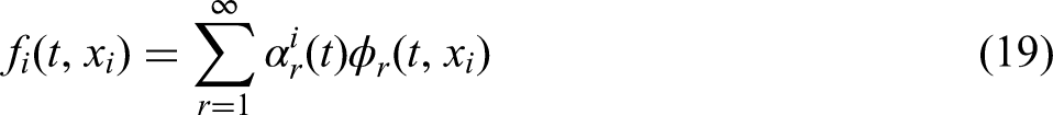

f_{i} (t, x_{i}) = \sum_{r = 1}^{\infty} α_{r}^{i} (t) ϕ_{r} (t, x_{i})

(19)

f_{i j} (x_{i}, x_{j}) = \sum_{p = 1}^{\infty} \sum_{q = 1}^{\infty} β_{p q}^{i j} (t) ϕ_{p q} (t, x_{i}, x_{j})

(20)Here,

ϕ_{r} (t, x_{i})

and

ϕ_{p q} (t, x_{i}, x_{j})

are the sets of one-dimensional and two-dimensional basis functions, where

α_{r}^{i} (t)

and

β_{p q}^{i j} (t)

are the coefficients of decomposition. According to the orthogonality of the basis function, it can be concluded that

α_{r}^{i} (t) = \int_{0}^{1} f_{i} (t, x_{i}) ϕ_{r} (t, x_{i}) d x_{i}, r = 1, \dots, k

(21)

\begin{aligned} β_{p q}^{i j} (t) = \int_{0}^{1} \int_{0}^{1} f_{i} (t, x_{i}) ϕ_{p} (t, x_{i}) ϕ_{q} (t, x_{j}) d x_{i} d x_{j} \\ p = 1, \dots, l, q = 1, \dots, l^{'} \end{aligned}

(22)

The choice of basis function is contingent upon the probability distribution of the input. For inputs that are uniformly distributed, the Legendre polynomial serves as the appropriate basis. Conversely, for arbitrary distributions, frequent practice involves applying variable transformations to convert a given distribution into a uniform distribution.³⁸

In practical applications, the summation range of equations (19) and (20) can be limited to some maximum orders k, $l$ , $l^{'}$ . Therefore, the high-dimensional model representation (HDMR) approximation function including only the first-order interaction and the second-order interaction can be constructed as

\tilde{f} (x) = f_{0} + \sum_{r = 1}^{k} α_{r}^{i} φ_{r} (t, x_{i}) + \sum_{p = 1}^{l} \sum_{q = 1}^{l^{'}} β_{p q}^{i j} (t) φ_{p} (t, x_{i}) φ_{q} (t, x_{j})

(23)

The error of the approximate model is measured by the Euclidean distance:

δ (f, \tilde{f}) = \frac{1}{σ} \int {[f (x) - \tilde{f} (x)]}^{2} d x

(24)

The least-squares method can be employed to select the optimal number of first-order and second-order polynomial terms for the approximate model. Additionally, the regression method can be utilised to estimate the decomposition coefficients of each polynomial.³⁹ The Sobol sensitivity index can then be evaluated using these decomposed coefficients⁴⁰:

S_{i} \approx \frac{\sum_{r = 1}^{k} {(α_{r}^{i})}^{2}}{σ^{2}}

(25)

S_{i j} \approx \frac{\sum_{p = 1}^{l} \sum_{ς = 1}^{l^{'}} {(β_{p q}^{i j})}^{2}}{σ^{2}}

(26)

S_{i}^{T} = S_{i} + \sum_{j = 1}^{n} S_{i j}

(27)In the above formulae, S_i is the main effect index,

S_{i}^{T}

is the total effect index, and S_ij is the high-order effect index, which reflects the influence of the interaction between multiple design parameters of the BIT circuit on the output variance.

Information fusion model of BIT module

As a complex RF circuit system, the BIT circuit exhibits characteristics of non-linearity and multivariable interaction, which significantly complicate sensitivity analysis. The necessity to account for physical device degradation and the time-dependent behaviour of the BIT circuit renders the computation of circuit responses via the BIT circuit simulation model highly time-consuming, thereby diminishing the efficiency of sensitivity analysis. In contrast, a BIT circuit surrogate model trained through machine learning can swiftly yield circuit responses, enhancing the efficiency of sensitivity analysis. Furthermore, a DNN is adept at managing the high-dimensional data inherent in complex circuit systems, effectively capturing the non-linear relationships among parameters and addressing uncertainties within circuit systems. Currently, a DNN is extensively used in RF circuit modelling, demonstrating high accuracy. Consequently, this paper employs a DNN to establish a surrogate model for the BIT circuit.

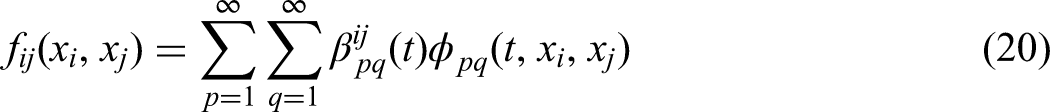
A DNN is a multi-layer, unsupervised neural network that contains multiple hidden layers positioned between the input layer and the output layer.⁴¹ In comparison to shallow neural networks, a DNN is more effective at capturing and expressing complex features and patterns.⁴² The structure of a DNN is illustrated in Figure 5.

Figure 5.

Structure of deep neural network (DNN).

Let $x = [x_{1} x_{2} x_{3} \dots x_{n}]^{T}$ represent the external input of a DNN model, where n is the number of model inputs. Let $y = [y_{1} y_{2} y_{3} \dots y_{m}]^{T}$ represent the output of the DNN model, where m is the number of model outputs and p is the number of hidden layers. The total number of layers of the DNN is $L = p + 2$ , including hidden layer, input layer, and output layer. Let l be the index of the network layer in the DNN, where $l = 1, 2, \dots, L$ . Let the output of each hidden layer and output layer of the DNN be $H_{l}$ , then:

H_{l} = f (W_{l} H_{l - 1} + b_{l}), l = 2, 3, \dots, L

(28)where f is the activation function,

W_{l}

is the weight matrix, and

b_{l}

is the bias. Let

F_{θ}

be the DNN of L-layer, then:

F_{θ} (x) = f_{L} (W_{L} \cdot f_{L - 1} (W_{L - 1} \cdot \cdot \cdot f_{1} (W_{1} \cdot x + b_{1}) \cdot \cdot \cdot + b_{L - 1}) + b_{L})

(29)where

θ

is the parameter set of the DNN. The training process of the DNN is a process of parameter fitting. By finding the optimal parameter

θ

, the difference between the real label and the predicted output is minimised. From a mathematical point of view, the training process of the DNN is equivalent to minimising the loss function

E (\cdot)

, as shown below:

θ = \underset{θ}{\arg min} \sum_{x^{i} \in χ} E (F_{θ} (x^{i}), y^{i})

(30)

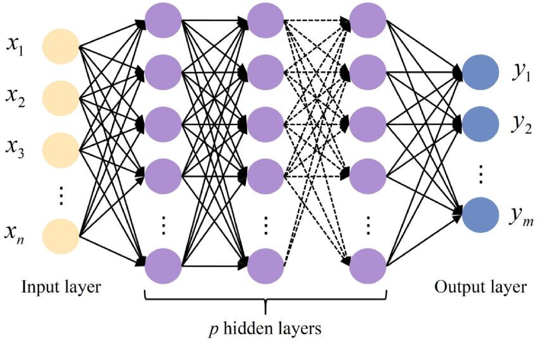
Among them, $χ$ is the training data set, $x^{i}$ is the training input sample, $y^{i}$ is the real label, and $F_{θ} (x^{i})$ is the prediction output.

The selection of activation function will affect the training quality of the DNN. The most common activation functions in conventional neural networks are smooth switch functions, such as the sigmoid function. The sigmoid function is shown in Figure 6(a) and expressed as

σ (γ) = \frac{1}{(1 + e^{- γ})}

(31)where

γ

denotes the total input to the hidden neuron.

Figure 6.

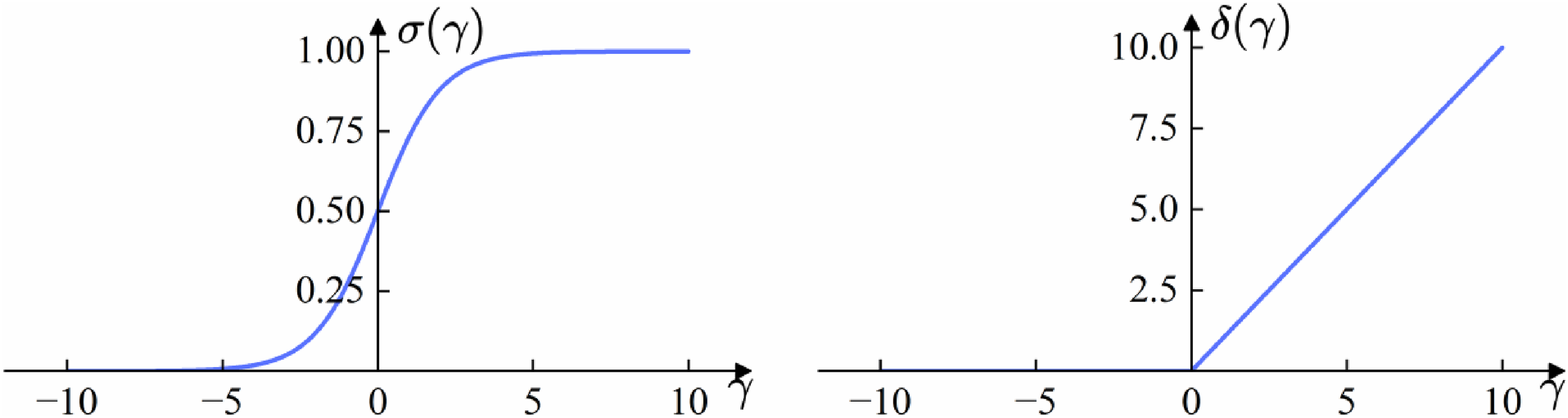
Two types of activation functions used in the hybrid deep neural network: (a) sigmoid function and (b) rectified linear unit (ReLU) function.

Shallow neural networks utilising sigmoid activation functions can typically be trained effectively using the gradient-based backpropagation algorithm from a random initialisation. However, training DNNs with sigmoid functions presents challenges due to the problem of gradient disappearance.⁴³ To overcome the problem of gradient disappearance during DNN training, the rectified linear unit (ReLU) has been developed as the activation function of the DNN. The ReLU is shown in Figure 6(b) and expressed as

δ (γ) = max (γ, 0) = {\begin{matrix} γ, if γ > 0 \\ 0, otherwise . \end{matrix}

(32)

When the total input $γ$ is greater than zero, the hidden layer neurons with ReLU activation are active.

The partial derivative of ReLU is always equal to 1 when active, allowing gradient information to be effectively propagated through active neurons in the DNN, thus avoiding gradient disappearance. The accuracy of the DNN depends on the quality and quantity of training data. The experimental data from the balise, derived from its actual output, ensures high-quality training data. However, this data is limited and results in a small sample size. On the other hand, physical knowledge data of the balise, abstracted from the real system, can be generated through numerical simulations, producing a large volume of sample data. To optimise the training dataset, it is crucial to integrate experimental data with physical knowledge data. The balise physical knowledge data is used for pre-training the DNN, followed by refining the model with balise experimental data to maximise the accuracy of the surrogate model.

Training the DNN model requires selecting initial values for model parameters. A pre-trained DNN model, based on physical knowledge, can mitigate issues related to poor initialisation due to insufficient understanding of initial parameter selection. Due to the varying complexities in obtaining output scalar characteristics between the ideal balise numerical calculation model and the actual BIT circuit simulation model, different sampling methods are necessary for generating input parameter samples. For the BIT circuit simulation model, a single-factor uniform sampling approach is used, systematically varying each input variable to generate experimental data under diverse conditions. For the balise numerical calculation model, LHS is employed to obtain physical knowledge data. LHS, an approximate RS technique for multivariate parameter distributions, allows accurate reconstruction of input distributions with fewer iterations. The key aspect of LHS is the stratification of the input probability distribution, dividing the cumulative curve into equal intervals along the cumulative probability scale (0, 1), and randomly selecting samples from each interval. This ensures that sampling results are evenly distributed across the sample space.

Uncertainty analysis of system model

While constructing a surrogate model can significantly reduce the computational cost associated with the sensitivity analysis of complex models, it inevitably introduces additional uncertainty to the results of the sensitivity analysis. In the sensitivity analysis of the BIT circuit surrogate model, it is essential not only to evaluate the uncertainty associated with the surrogate model but also to provide a reasonable explanation of its engineering significance.

To quantify the impact of uncertainty in the BIT circuit surrogate model on the results of sensitivity analysis, a Monte Carlo (MC) dropout regularisation method can be employed to generate uncertain outputs from identical inputs. MC dropout involves the random omission of neurons and their connections with a specified ‘dropout probability’ during the training and prediction phases of the DNN, thereby simulating model uncertainty.⁴⁴ In terms of methodological application, MC dropout serves to mitigate overfitting in the DNN model and reduce generalisation error. From an engineering perspective, it effectively simulates individual differences within the same batch of products. Under identical design parameters, this approach allows for the generation of multiple distinct output results from a single batch of products.

The uncertainty present in the DNN model can be propagated to the sensitivity calculations through the following estimators⁴⁵:

S_{m}^{D N N} = \frac{(1 / m) \sum_{k = 1}^{m} ς^{\hat{ω}} (X_{k}) ς^{\hat{ω}} ({X^{'}}_{k}) - (1 / m) \sum_{k = 1}^{m} ς^{\hat{ω}} (X_{k}) \sum_{k = 1}^{m} ς^{\hat{ω}} ({X^{'}}_{k})}{(1 / m) \sum_{k = 1}^{m} ς^{\hat{ω}} {(X_{k})}^{2} - (1 / m) \sum_{k = 1}^{m} {(ς^{\hat{ω}} (X_{k}))}^{2}}

(33)where

ζ^{\hat{ω}} (X_{k})

represents the DNN model that utilises the MC dropout function,

X_{k}

and

X_{k}^{'}

are the k-th random sampling of the input vectors X and

X^{'}

. The DNN model will execute MC dropout

N_{d}

times under the k-th input vector to generate

N_{d}

model outputs, thereby producing N_d instances of

S_{m}^{D N N}

. The mean and variance of the uncertainty in the DNN model can be expressed as follows:

μ_{S_{m}^{D N N}} = \frac{1}{N_{d}} \sum_{p = 1}^{N_{d}} {\hat{S}}_{m, p}^{D N N}

(34)

σ_{S_{m}^{D N N}}^{2} = \frac{1}{N_{d}} \sum_{p = 1}^{N_{d}} {({\hat{S}}_{m, p}^{D N N} - μ_{S_{m}^{D N N}})}^{2}

(35)

By introducing the MC dropout method to quantify model uncertainty, the sensitivity analysis shifts from relying on a single deterministic output to using the statistical results derived from multiple inferences. Consequently, the outcome of the sensitivity analysis is no longer confined to a single value; instead, it encompasses a range of possible values. This quantification of model uncertainty enhances the reliability and robustness of sensitivity analysis, particularly for complex systems characterised by uncertainty.⁴⁶

Experiments

Dataset description

Parameters of the surrogate model

The BIT circuit model illustrated in Figure 2 is idealised, omitting the series resistance between the equivalent inductors L₁ and L₂. To accurately simulate the discrepancies between the physical knowledge data and the experimental data, series resistors R_a, R_b, and additional auxiliary circuits have been incorporated between V_n and V_p. The modified section of the BIT circuit is depicted in Figure 7.

Figure 7.

Modified section of the balise information transmitting (BIT) circuit.

Ten input parameters and five output parameters are selected as model parameters, as shown in Table 2.

Table 2.

Input and output parameters of the BIT circuit model.

Input parameter	Design parameter	Input parameter	Design parameter	Output parameter
(x₁) L₁, L₂	1.32 (μH)	(x₆) C₈, C₉	800 (pF)	(y₁) Centre frequency
(x₂) C₁, C₂	56 (pF)	(x₇) R₁, R₂	68 (kΩ)	(y₂) Frequency deviation
(x₃) C₃, C₄	56 (pF)	(x₈) R₃	100 (kΩ)	(y₃) Mean data rate
(x₄) C₅, C₆	355 (pF)	(x₉) Beta	303	(y₄) Signal bandwidth
(x₅) C₇	35 (pF)	(x₁₀) V_dd	5 (V)	(y₅) Signal amplitude

BIT: balise information transmitting.

In Table 2, Beta represents the current gain of the BJT. The values of the magnetic field model parameters utilised in the numerical calculation model, along with the circuit simulation model and additional circuit components not included in the model input parameters of the circuit simulation, are detailed in Table 3.

Table 3.

Other model parameters of the balise.

Simulation parameter	Parameter value	Simulation parameter	Parameter value
Size of information transmitting antenna	200 × 390 mm	Size of train-mounted antenna	200 × 200 mm
Quality factor of train-mounted antenna	10	Matching impedance of train-mounted antenna	50 Ω
Balise telegram	Test telegram 9	The height of the antenna relative to the balise	220 mm
Number of test telegrams sent	Two groups of 2048 bits	Sampling rate of data processing unit	200 MHz
$R_{a}$ , singledollarR_bsingledollar	5 (Ω)	$L_{f}$	40 (mH)
$C_{a}$	4.7 (pF)	$C_{b}$	2.2 (nF)

Training data of the surrogate model

The physical knowledge data utilised for training the BIT circuit surrogate model is derived from LHS conducted on the physical device degradation interval, which is subsequently fed into the balise numerical calculation model. It is assumed that the input parameters follow a normal distribution, with the design parameter value representing the mean and the variance being determined by the $3 σ$ criteria. The accuracy of the input parameters x₁ to x₉ is set at 5%, while the accuracy of x₁₀ is set at 2%. It is assumed that the influence of external force impacts and the output of the balise energy-receiving circuit on the BIT circuit is not considered. Based on the physical degradation model of the inductor, it can be assumed that inductance remains unchanged. The total degradation of capacitance is approximately 1%, the total degradation of resistance is around 5%, the total degradation of the BJT is about 45%, and the total degradation of the LDO regulator is approximately 5%.

The experimental data utilised for training the BIT circuit surrogate model was obtained through single-factor uniform sampling across the degradation interval of the physical device, which was subsequently input into the actual balise circuit model. The sampling intervals for input parameters x₁ to x₈ ranged from 90% to 110% of the design parameters, while the sampling interval for x₉ spanned from 50% to 150% of the design parameters, and for x₁₀, it was set between 98% and 102% of the design parameters. The sampling interval encompasses the sum of the initial tolerance and the degradation tolerance for each parameter. Since the physical knowledge data and the experimental data used to train the surrogate model include the degradation tolerance of the physical device influenced by environmental factors, the surrogate model inherently accounts for these environmental factors.

To reflect the small sample nature of the experimental data and to verify the impact of varying sample sizes on the DNN model, single-factor uniform sampling was conducted with three to four samples for each input parameter. In total, 35 samples are generated, from which 5, 10, 15, 20, and 25 samples are selected to update the DNN model, leaving the remaining 10 samples for model verification.

Deterioration input of the surrogate model

When analysing the sensitivity of the BIT circuit surrogate model, the deterioration data should be utilised as the input to obtain the scalar output of the model. For the initial tolerance setting of parameter deterioration, 5000 input samples for the BIT circuit surrogate model are generated using Sobol sampling. Assuming that the input parameters follow a normal distribution, the mean represents the design parameter, while the variance is determined according to the $3 σ$ criterion. The accuracy of the input parameters x₁ to x₉ is set at 5%, whereas the accuracy of x₁₀ is set at 2%.

In the degradation tolerance setting for parameter deterioration, the degradation period is established at 10 years. The effects of external force impacts and the output of the balise energy-receiving circuit on the BIT circuit are not considered. The total degradation of the capacitance is approximately 1%, the total degradation of the resistance is about 5%, the total degradation of the BJT is around 45%, and the total degradation of the LDO regulator is about 5%, excluding the degradation of inductance.

A total of 5000 samples were utilised to simulate the individual differences of different balise circuits with initial tolerances. Based on the degradation model of each physical device within the BIT circuit, the corresponding parameter values for each sample over a 10-year period were generated, denoted T₁ to T₁₀. Using the deterioration input and output of the BIT circuit surrogate model at different time points, the RS-HDMR method was employed to compute the sensitivity index at each moment.

Difference analysis of data generation models

The physical knowledge data for training the surrogate model is generated using the balise numerical calculation model, while the experimental data is derived from the balise circuit simulation model. This section aims to analyse and verify the effectiveness of both models in characterising the differences between physical knowledge data and experimental data. Utilising the modified BIT circuit simulation model, a single-factor uniform sampling experiment is conducted for each input parameter, allowing for a qualitative analysis of the discrepancies between the numerical calculation model and the circuit simulation model. For each input parameter, 41 sample points are evenly distributed. The sampling intervals for input parameters x₁ to x₈ range from 90% to 110% of the design parameters, while the sampling interval for x₉ spans from 50% to 150% of the design parameters, and x₁₀ is sampled within the range of 98% to 102% of the design parameters. The results of the z-score normalisation of the model output are illustrated in Figure 8.

Figure 8.

Input and output correlation analysis of the circuit simulation model.

Figure 8 illustrates that all the parameters, with the exception of R₃, exhibit a relationship with the outputs.

The output y₁, y₂, and y₃ are similar to the correlation of other input parameters except for the correlation with x₄. A negative correlation exists between y₁, y₃, and x₄, with Pearson coefficients of −0.9842 and −0.9880, respectively. In contrast, y₂ shows no significant correlation with x₄, as indicated by a Pearson coefficient of only −0.0524. A strong negative correlation is observed between y₁, y₂, y₃, and x₁, x₆, with their Pearson coefficients being less than −0.9796. Additionally, there is a negative correlation between y₁, y₂, y₃, and x₃, x₅, with Pearson coefficients ranging from −0.6083 to −0.7164. A degree of negative correlation is also present between y₁, y₂, y₃, and x₂, x₇, x₁₀, with Pearson coefficients between −0.4350 and −0.5203. This indicates that the output frequency characteristics of the balise are influenced not only by the LC resonant circuit but also by the cross-coupling circuit, thereby indirectly validating the accuracy of the numerical calculation model analysis of the balise. However, the circuit simulation model also concludes that the output frequency exhibits a certain negative correlation with R₁, R₂, and V_dd, highlighting a cognitive oversight in the numerical calculation model that fails to account for these factors.

The output y₄ exhibits a strong correlation with both x₄ and x₅, with Pearson coefficients of 0.9628 and −0.8161, respectively. Additionally, a negative correlation exists between y₄ and both x₆ and x₁₀, with Pearson coefficients of −0.5402 and −0.4684, respectively. This indicates that the fluctuations in signal bandwidth are strongly correlated with C₅, C₆, and C₇. This correlation is fundamentally attributed to the changes in frequency during the transmission of balise telegrams, which leads to variations in signal bandwidth. Furthermore, due to the differences in output frequencies, the balise numerical calculation model and the circuit simulation model are likely to exhibit certain cognitive discrepancies in signal bandwidth.

The output y₅ exhibits a strong correlation with eight input parameters, demonstrating positive correlations with x₁, x₃, x₉, and x₁₀, with Pearson coefficients of 0.9883, 0.9912, 0.9702, and 0.9629, respectively. Conversely, it shows negative correlations with x₂, x₄, x₆, and x₇, with Pearson coefficients of −0.9693, −0.9966, −0.9877, and −0.9995, respectively. The Pearson coefficient with x₅ is low at 0.2132. This indicates that the signal amplitude is strongly correlated with other input parameters, except for C₆ and R₃, and is influenced by the parameters of multiple physical devices. Although the numerical calculation model of the balise can characterise this correlation, it does not account for the relationships between the signal amplitude and R₁, R₂, and Beta. Therefore, a cognitive discrepancy remains when compared to the circuit simulation model.

The above analysis primarily analyses the relationship between the input parameters and the output parameters of the modified BIT circuit simulation model from the perspective of linear correlation. However, a strong correlation does not necessarily imply a higher sensitivity index between the input and output. For instance, the Pearson correlation coefficient between output y₄ and input x₁ is merely −0.0967. Nevertheless, an examination of volatility reveals that the influence of x₁ on the fluctuations of outputs y₁, y₂, y₃, and y₅ is less significant than its influence on y₄.

In summary, although the numerical calculation model can characterise the relationship between the input and output of the BIT circuit, there exists a cognitive deviation when compared to the circuit simulation model. This indicates that the two models can effectively characterise the difference between physical knowledge data and experimental data.

Verification analysis of the surrogate model

To analyse the influence of various training datasets on the accuracy of the BIT circuit surrogate model, six distinct BIT circuit surrogate models have been designed. The root mean square error serves as the metric for comparing the performance of these different models. DNN^exp is derived from training on experimental data. The models DNN1^upd, DNN2^upd, DNN3^upd, DNN4^upd, and DNN5^upd are pre-trained using 1500, 2000, 2500, 3000, and 5000 groups of physical knowledge data, respectively, after which the pre-training models are updated with experimental data. The fully connected DNN model consists of two hidden layers, each containing 15 neurons. The ReLU activation function and the Adam optimiser are employed to conduct 300 cycles of stochastic gradient descent on the model parameters.

Various experimental datasets with n = (5, 10, 15, 20, 25) are utilised to assess the accuracy of different DNN models. The experimental results are presented in Table 4.

Table 4.

Influence of different training sets on the accuracy of the DNN model.

Surrogate model	Index	n = 5	n = 10	n = 15	n = 20	n = 25
DNN^exp	RMSE	0.400	0.341	0.359	0.348	0.296
DNN1^upd	RMSE	0.401	0.265	0.262	0.243	0.242
DNN2^upd	RMSE	0.403	0.318	0.326	0.296	0.274
DNN3^upd	RMSE	0.459	0.369	0.364	0.322	0.280
DNN4^upd	RMSE	0.415	0.341	0.295	0.286	0.277
DNN5^upd	RMSE	0.560	0.354	0.340	0.315	0.286

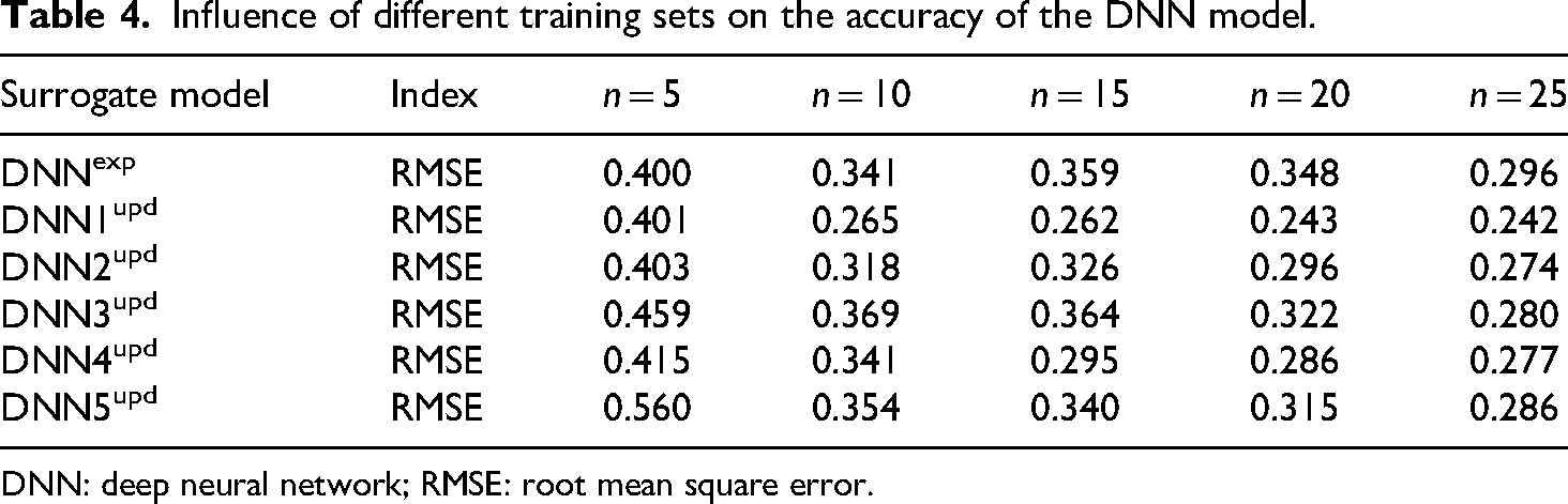
DNN: deep neural network; RMSE: root mean square error.

The results presented in Table 4 indicate that the accuracy of the DNN^upd model, which is trained through a combination of physical knowledge data pre-training and experimental data updating, surpasses that of the DNN model trained solely on experimental data. It is observed that the accuracy of all DNN models improves with an increase in the number of experimental samples. However, due to the inherent differences between physical knowledge data and experimental data, the accuracy of the DNN^upd model decreases as the number of physical knowledge samples increases during pre-training. Notably, while the decreasing trend persists, it tends to decelerate with an increase in the number of experimental samples. Table 4 illustrates that the DNN1^upd model, which utilises 1500 physical knowledge samples for pre-training and 25 experimental samples for updating, achieves the highest accuracy, thereby designating it as the BIT circuit surrogate model.

Furthermore, all DNN models are updated using 25 experimental samples, and the impact of varying dropout rates on the DNN model is analysed and compared, with the results detailed in Table 5.

Table 5.

Influence of dropout rate on the accuracy of the DNN model.

Surrogate model	Index	D = 0.005	D = 0.01	D = 0.05	D = 0.1	D = 0.2	D = 0.3	D = 0.4	D = 0.5
DNN^exp	RMSE	0.289	0.291	0.289	0.296	0.312	0.315	0.332	0.347
DNN1^upd	RMSE	0.259	0.257	0.255	0.242	0.251	0.258	0.266	0.267
DNN2^upd	RMSE	0.281	0.275	0.264	0.255	0.278	0.281	0.283	0.274
DNN3^upd	RMSE	0.254	0.256	0.241	0.261	0.270	0.272	0.297	0.280
DNN4^upd	RMSE	0.261	0.257	0.250	0.249	0.249	0.262	0.262	0.277
DNN5^upd	RMSE	0.265	0.261	0.255	0.255	0.271	0.281	0.286	0.286

DNN: deep neural network; RMSE: root mean square error.

Table 5 illustrates that as the dropout rate increases, the accuracy of all DNN models initially decreases before subsequently increasing. At a dropout rate of 0.1, the DNN1^upd model achieves the highest accuracy, indicating that the optimal dropout rate for this model is 0.1.

Comparative analysis of sensitivity methods

To verify the correctness and effectiveness of various sensitivity-solving methods, the RS-HDMR meta-model method, Bayesian sparse polynomial chaos expansion (BSPCE) meta-model method and Saltelli method are employed to compute the sensitivity index of the balise numerical calculation model. A total of 1500, 2000, 2500, 3000, and 5000 input samples are obtained through sampling, adhering to the requirements of different solution methods. The balise numerical calculation model is utilised to generate various combinations of output samples. Based on the input and output results from the numerical calculation model, the three solving methods are applied to determine the sensitivity index, followed by a comparative analysis of the methods in terms of time cost and calculation results.

Data collection is conducted using MATLAB for the Saltelli method, while RS-HDMR and BSPCE methods are solved utilising SobolGSA software, which operates on a general GUI driver. Data processing is executed on a system equipped with an Intel^® Core™ i7-8565U CPU at 1.80 GHz, 8 GB RAM, and NVIDIA GeForce MX250 with 2 GB VRAM; data collection is performed on a system with an Intel^® Core™ i9-9900 CPU at 3.10 GHz, 32 GB RAM, and NVIDIA GeForce GTX1060 with 6 GB VRAM. The time consumption of the three sensitivity analysis methods is illustrated in Figure 9.

Figure 9.

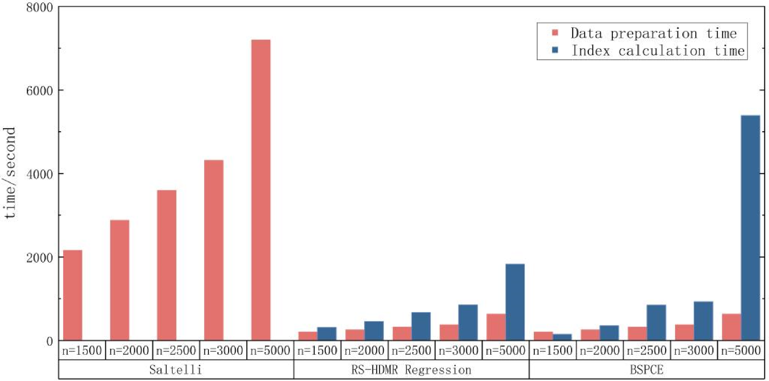
Time cost comparison of three sensitivity-solving methods.

The results presented in Figure 9 indicate that the time cost associated with the two meta-model methods is lower than that of the Saltelli method when analysing the same samples. This is primarily attributed to the reduced time required for data collection by the two meta-model approaches. To illustrate the difference in computational time between the two meta-model methods, the calculation process depicted in the figure employs a general GUI driver to resolve the correlation function. When the number of samples is fewer than 3000, the computational time for both meta-model methods does not significantly differ; however, with a larger sample size, the RS-HDMR method demonstrates a considerable advantage in terms of time efficiency. Based on the RS-HDMR method, the fluctuation range of the sensitivity index for all input parameters concerning output y₁, as well as the sensitivity index of all input parameters for all outputs, is calculated and presented in Figure 10.

Figure 10.

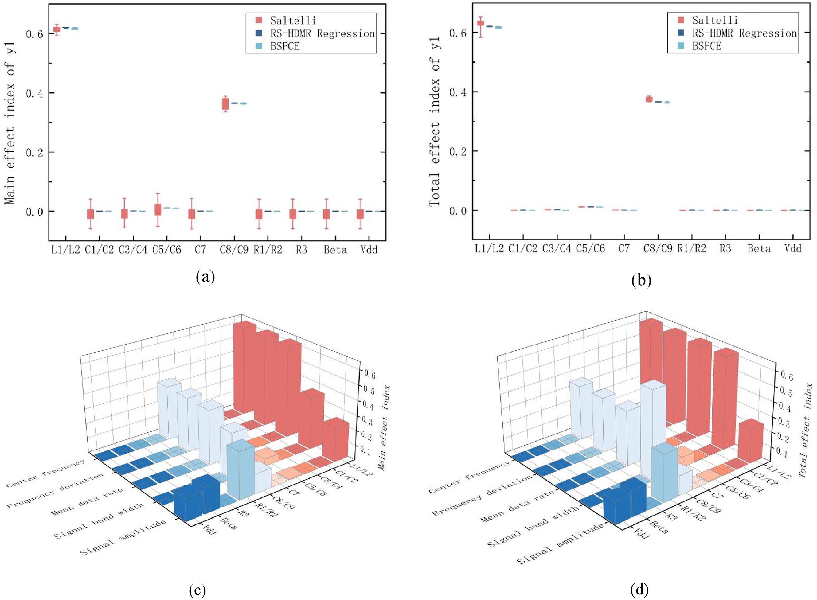
Sensitivity solution results of the random sampling-high-dimensional model representation (RS-HDMR) method: (a) the main effect index of y₁, (b) the total effect index of y₁, (c) the main effect index of all outputs, and (d) the total effect index of all outputs.

Figure 10(a) and (b) presents the sensitivity calculation results of output y₁ when analysing different samples, while Figure 10(c) and (d) illustrates the sensitivity calculation results between all inputs and outputs with a sample size of 5000. The sensitivity index fluctuation range for the Saltelli method, as the number of samples varies, is between 0.036 and 0.055. In contrast, the fluctuation range for the two meta-model methods is significantly narrower, ranging from 0.004 to 0.005. Notably, the sensitivity results obtained through the meta-model method are comparable to those of the Saltelli method. Furthermore, the modified numerical calculation model effectively reflects the correlation between input and output parameters. In conclusion, the RS-HDMR method demonstrates substantial advantages in both calculation accuracy and time efficiency, making it a viable approach for solving sensitivity indices.

Sensitivity analysis of performance degradation

The BIT circuit surrogate model utilising the dropout strategy generates a total of 5000 × 5 × 100 output groups when provided with 5000 input samples. Here, 5000 represents the number of samples, 5 indicates the number of output scalars, and 100 denotes the groups of uncertain outputs produced by the dropout strategy for each scalar output. When the initial tolerance leads to a degradation in output performance, the sensitivity index calculations for all input parameters of the BIT circuit concerning all output parameters are illustrated in Figure 11. Each sensitivity index in Figure 11 represents the mean value derived from 100 sets of uncertain outputs.

Figure 11.

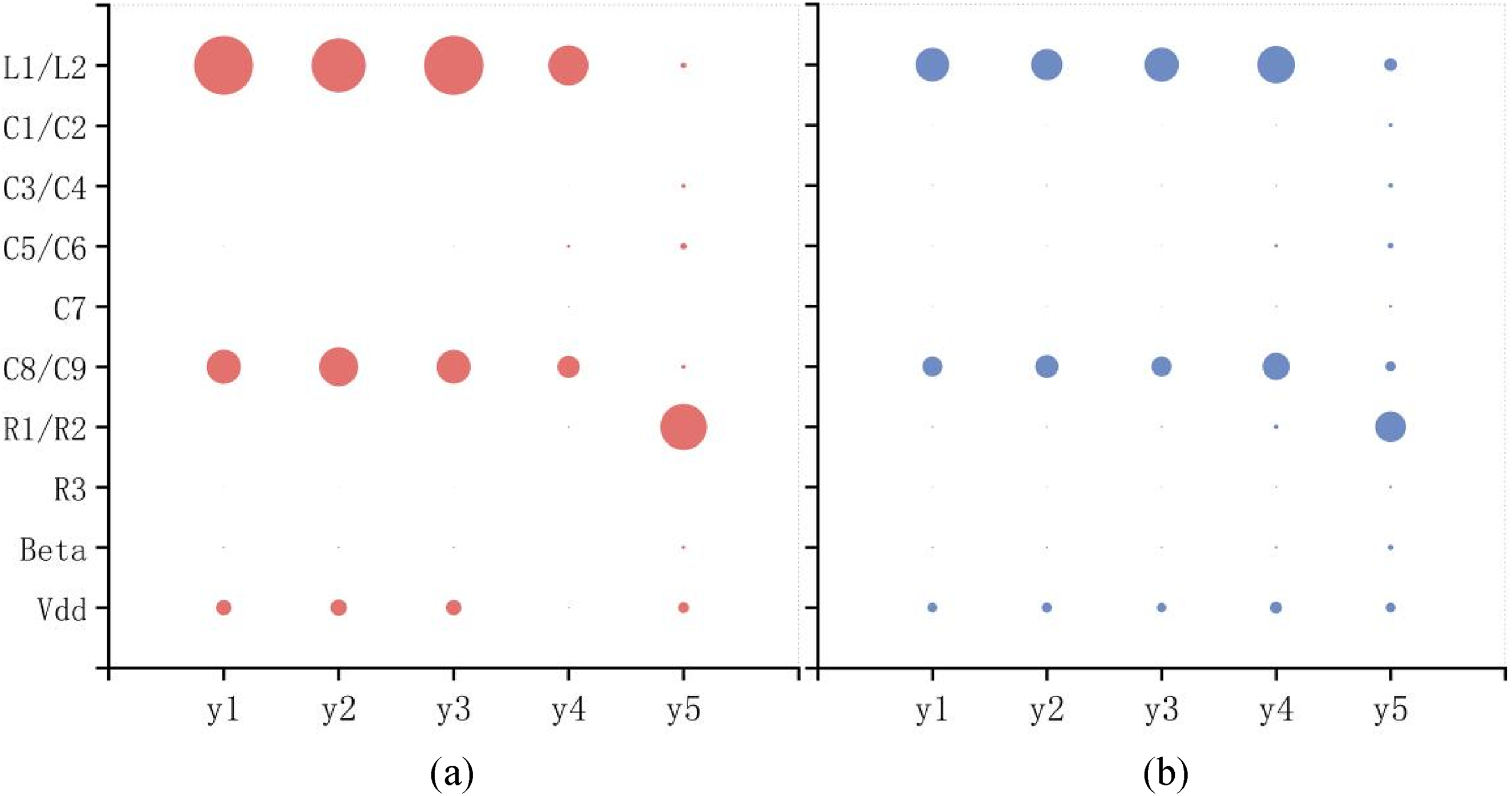
Sensitivity index of balise information transmitting (BIT) circuit under initial tolerance: (a) the main effect index of all outputs and (b) the total effect index of all outputs.

The main effect index indicates that the fluctuations in centre frequency, frequency offset, and average data rate are primarily influenced by L₁/L₂, C₈/C₉, and V_dd. In contrast, the signal bandwidth is most affected by L₁/L₂ and C₈/C₉, while the signal amplitude is most significantly impacted by R₁/R₂. When examining the total effect index, L₁/L₂, C₈/C₉, and V_dd exhibit similar sensitivities to centre frequency, frequency offset, average data rate, and signal bandwidth, while also affecting signal amplitude. Consequently, during the balise circuit design and tolerance analysis phase, it is crucial to prioritise the accuracy of L₁/L₂, C₈/C₉, R₁/R₂, and V_dd.

When initial tolerances lead to a decline in output performance, the fluctuations in the sensitivity analysis results are illustrated in Figure 12. This figure depicts the range of fluctuations for each effect index, which reflects 100 sets of fluctuation outputs generated due to model uncertainty.

Figure 12.

Fluctuation of sensitivity index under initial tolerance: (a) the main effect index of y₁, (b) the total effect index of y₁, (c) the main effect index of y₂, (d) the total effect index of y₂, (e) the main effect index of y₃, (f) the total effect index of y₃, (g) the main effect index of y₄, (h) the total effect index of y₄, (i) the main effect index of y₅, and (j) the total effect index of y₅.

From Figure 12(a) and (b), it is evident that MC dropout reflects the uncertainty of the BIT circuit surrogate model through a normal distribution in the sensitivity index results. A smaller mean value of the sensitivity index corresponds to reduced fluctuation, indicated by a smaller standard deviation and a larger coefficient of variation (the ratio of standard deviation to mean). For instance, the mean value of the main effect index of y₁ for L₁/L₂ is 0.47, with a standard deviation of 0.0041 and a coefficient of variation of 8‰. In contrast, the mean value of the main effect index of y₁ for V_dd is 0.12, with a standard deviation of 0.0032 and a coefficient of variation of 25‰.

When the degradation tolerance of the overall batch balise leads to a degradation in output performance, the results of the sensitivity analysis are presented in Figure 13. In this figure, each effect index represents the mean of 100 sets of uncertain outputs.

Figure 13.

Sensitivity index of the overall batch balise under degradation tolerance: (a) the main effect index of y₁, (b) the total effect index of y₁, (c) the main effect index of y₂, (d) the total effect index of y₂, (e) the main effect index of y₃, (f) the total effect index of y₃, (g) the main effect index of y₄, (h) the total effect index of y₄, (i) the main effect index of y₅, and (j) the total effect index of y₅.

Figure 13 illustrates that the standard deviation of all effect indices is less than 0.003, the coefficient of variation is below 2%, and the range is also under 2%. In comparison to the initial tolerance of 100 groups of effect indices, the standard deviation, coefficient of variation, and range of the 10 groups of mean effect indices of degradation tolerance exhibit a temporal decrease. Furthermore, the maximum and minimum values of the 100 groups of initial tolerance effect indices, based on MC dropout, encompass the maximum and minimum values of each effect index pertaining to degradation tolerance. This suggests that the degradation tolerance of input parameters has a minimal impact on both the main effect index and the total effect index of each output scalar feature of the balise.

When the degradation tolerance of a single balise leads to a decline in its output performance, the results of the sensitivity analysis are presented in Figure 14. In this figure, each effect index represents the mean of 100 sets of uncertain outputs.

Figure 14.

Sensitivity index of the individual balise under degradation tolerance: (a) the main effect index of all outputs and (b) the total effect index of all outputs.

The individual balise does not account for inductance degradation, and its outputs y₁ to y₄ remain significantly influenced by the input parameters C₈/C₉ and V_dd. This observation aligns with the sensitivity analysis results of the overall batch balise. However, the factors influencing the output y₅ differ. Based on the results of various performance degradation analyses, C₈/C₉, R₁/R₂, and the LDO regulator can be identified as the critical electronic components affecting the performance degradation of the balise.

Conclusion

This paper proposes a sensitivity analysis method for the BIT circuit that accounts for performance degradation and model uncertainty. By selecting an appropriate scalar output and discretising the dynamic model of the BIT circuit, a surrogate model based on DNNs is established, integrating both physical knowledge and experimental data. An RS-HDMR method is employed to analyse the sensitivity of the BIT circuit surrogate model, identifying the key physical devices contributing to the performance degradation of the BIT circuit. The effectiveness of this method is validated through experiments, which demonstrate that the capacitance C₈/C₉, resistance R₁/R₂, and LDO regulator are the critical components affecting performance degradation of the BIT circuit. Integrating physical knowledge with experimental data significantly enhances the accuracy of the surrogate model. Compared to other sensitivity analysis methods, the RS-HDMR method demonstrates superior computational accuracy and efficiency. However, challenges remain in applying the RS-HDMR method to other complex dynamic models. In the future, it is recommended to explore ways to optimise the RS-HDMR method for broader application in more complex dynamic systems, and to investigate whether there are more suitable sensitivity analysis methods for various railway equipment.

This study has proposed a theoretical reference for the design and maintenance of the BIT circuit from the perspective of physical devices. Optimising the design of balise at the system level based on the analysis results obtained from the physical device level is also a promising direction for future research.

Footnotes

Acknowledgements

The authors would like to acknowledge the support of the China Scholarship Council for facilitating collaborative research. Special thanks are extended to Professor Roger Dixon from the University of Birmingham for his insightful guidance and valuable suggestions during the revision of the manuscript.

ORCID iD

Zhengjiao Li

Jiang Liu

Funding

The authors disclosed receipt of the following financial support for the research, authorship, and/or publication of this article: This work was supported by the China Scholarship Council, Fundamental Research Funds for the Central Universities, National Natural Science Foundation of China (grant numbers 2024JBMC034, 52102472, T2222015, U2268206).

Declaration of conflicting interests

The authors declared no potential conflicts of interest with respect to the research, authorship, and/or publication of this article.

References

Cai

Liu

, et al. Modelling and performance analysis of balise under dynamic energy harvesting in high-speed railway. IET Intel Transport Syst 2022; 16: 1504–1520.

Jinhua

. Railway vehicle fault intelligent maintenance system based on association mining. In: 2019 11th International Conference on Measuring Technology and Mechatronics Automation (ICMTMA), Qiqihar, China, 28–29 April 2019, pp. 182–186.

Chen

Jiang

, et al. Latest progress on maintenance strategy of complex system: from condition-based maintenance to predictive maintenance. Acta Autom Sin 2021; 47: 1–17.

Naseh

Deen

Marinov

. Effects of hot-carrier stress on the performance of the LC-tank CMOS oscillators. IEEE Trans Electron Devices 2003; 50: 1334–1339.

Saarinen

Frisk

. Reliability analysis of UHF RFID tags under a combination of environmental stresses. IEEE Trans Device Mater Reliab 2013; 13: 119–125.

Kang

Lee

Kim

, et al. Remaining useful life estimation using accelerated degradation test, a gamma process, and the Arrhenius model for nuclear power plants. J Mech Sci Technol 2022; 36: 4905–4912.

Keimasi

Azarian

Pecht

. Isothermal aging effects on flex cracking of multilayer ceramic capacitors with standard and flexible terminations. Microelectron Reliab 2007; 47: 2215–2225.

Liu

Zhang

, et al. An improved lifetime prediction method for metallized film capacitor considering harmonics and degradation process. Microelectron Reliab 2020; 114: 113892.

Paulsen

Reed

. Highly accelerated life testing of base-metal-electrode ceramic chip capacitors. Microelectron Reliab 2002; 42: 815–820.

10.

Zhao

You

. Failure analysis of multi-layer ceramic capacitors under board level shock environment. In: 2018 IEEE International Conference on Electron Devices and Solid State Circuits (EDSSC), Shenzhen, China, 6–8 June 2018, pp. 1–2.

11.

Wang

Qiu

Chen

, et al. Machine learning-based analyses for total ionizing dose effects in bipolar junction transistors. Nucl Sci Tech 2022; 33: 131.

12.

Liu

Sun

Wang

, et al. Characterizing and modeling current gain degradation in bipolar transistor exposed to heavy ion radiation. Mater Sci Semicond Process 2021; 121: 105336.

13.

Lin

Yam

RCM

. Uncertainty importance measures of dependent transition rates for transient and steady state probabilities. Reliab Eng Syst Saf 2017; 165: 402–409.

14.

Saltelli

. Sensitivity analysis for importance assessment. Risk Anal 2002; 22: 579–590.

15.

Zhang

Xiao

, et al. A dynamic time evolution method for concurrent device-circuit aging simulations. IEEE Trans Electron Devices 2019; 66: 184–190.

16.

Zhu

Wang

, et al. Sensitivity analysis of inductive power transfer systems with voltage-fed compensation topologies. IEEE Trans Veh Technol 2019; 68: 4502–4513.

17.

Saltelli

Aleksankina

Becker

, et al. Why so many published sensitivity analyses are false: a systematic review of sensitivity analysis practices. Environ Model Softw 2019; 114: 29–39.

18.

Borgonovo

Plischke

. Sensitivity analysis: a review of recent advances. Eur J Oper Res 2016; 248: 869–887.

19.

Saltelli

Ratto

Andres

, et al. Global sensitivity analysis: the primer. 1st ed. Chichester: John Wiley & Sons, 2007.

20.

Sobol

. Global sensitivity indices for nonlinear mathematical models and their Monte Carlo estimates. Math Comput Simul 2001; 55: 271–280.

21.

Zhang

Cheng

, et al. Global sensitivity analysis for multivariate output model and dynamic models. Reliab Eng Syst Saf 2020; 204: 107195.

22.

Campbell

McKay

Williams

. Sensitivity analysis when model outputs are functions. Reliab Eng Syst Saf 2006; 91: 1468–1472.

23.

Lamboni

Monod

Makowski

. Multivariate sensitivity analysis to measure global contribution of input factors in dynamic models. Reliab Eng Syst Saf 2011; 96: 450–459.

24.

Barton

Meckesheimer

. Metamodel-based simulation optimization. Handb Oper Res Manage Sci 2006; 13: 535–574.

25.

Pinedo

Aguado

Rodriguez

, et al. Near-field wireless communications and their role in next generation transport infrastructures: an overview of modelling techniques. In: Hilt B, Berbineau M, Vinel A, et al. Networking Simulation for Intelligent Transportation Systems. Wiley Telecom, 2017, pp. 29–50.

26.

Dabbaghzadeh

Falahati

Sanandaji

. CBTC security and reliability enhancements by a key-based direct sequence spread Spectrum technique. IEEE Trans Intell Transp Syst 2024; 25: 159–172.

27.

Zhao

Liu

, et al. A magnetic field-circuit coupling model for functionality and interface simulation test of railway balise. Adv Mech Eng 2023; 15: 16878132231188821.

28.

Moghavvemi

Attaran

. Performance review of high-quality-factor, low-noise, and wideband radio-frequency LC-VCO for wireless communication. IEEE Microwave Mag 2011; 12: 130–146.

29.

Thakkar

Theertham

Mirajkar

, et al. A 27.2 GHz bipolar LC-VCO using class-C biasing to maximize achievable FOSC in 130 nm BiCMOS. In: 2018 IEEE International Symposium On Circuits And Systems (ISCAS), Florence, Italy, 27–30 May 2018, pp. 1–5.

30.

Zhai

Zhou

. A tolerance design method for electronic circuits based on performance degradation. Qual Reliab Eng Int 2013; 31: 635–643.

31.

Geng

Wen

Zhang

, et al. Analysis of electromagnetic coupling characteristics of balise transmission system based on digital twin. Appl Sci 2021; 11: 6002.

32.

Zheng

, et al. Degradation mechanisms-based reliability modeling for metallized film capacitors under temperature and voltage stresses. Microelectron Reliab 2022; 138: 114609.

33.

Zheng

Chen

Lin

, et al. Optimal design of step-stress accelerated degradation test oriented by nonlinear and distributed degradation process. Reliab Eng Syst Saf 2022; 217: 108087.

34.

Maricau

De Wit

Gielen

. An analytical model for hot carrier degradation in nanoscale CMOS suitable for the simulation of degradation in analog IC applications. Microelectron Reliab 2008; 48: 1576–1580.

35.

Subramanian

Mahadevan

. Variance-based sensitivity analysis of dynamic systems with both input and model uncertainty. Mech Syst Signal Process 2022; 166: 108423.

36.

Rabitz

, et al. Regularized random-sampling high dimensional model representation (RS-HDMR). J Math Chem 2007; 43: 1207–1232.

37.

Wang

, et al. Random sampling-high dimensional model representation (RS-HDMR) and orthogonality of its different order component functions. J Phys Chem A 2006; 110: 2474–2485.

38.

Zuniga

Kucherenko

Shah

. Metamodelling with independent and dependent inputs. Comput Phys Commun 2013; 184: 1570–1580.

39.

Spiessl

Kucherenko

Becker

D-A

, et al. Higher-order sensitivity analysis of a final repository model with discontinuous behaviour using the RS-HDMR meta-modeling approach. Reliab Eng Syst Saf 2019; 187: 149–158.

40.

Wang

Rabitz

, et al. Global uncertainty assessments by high dimensional model representations (HDMR). Chem Eng Sci 2002; 57: 4445–4460.

41.

Bengio

. Learning deep architectures for AI. Found Trends Mach Learn 2009; 2: 1–127.

42.

Szegedy

Toshev

Erhan

. Deep neural networks for object detection. Adv Neural Inf Process Syst 2013; 26.

43.

Bengio

Simard

Frasconi

. Learning long-term dependencies with gradient descent is difficult. IEEE Trans Neural Netw 1994; 5: 157–166.

44.

Rodriguez-Puigvert

Martinez-Cantin

Civera

. Bayesian deep neural networks for supervised learning of single-view depth. IEEE Robot Autom Lett 2022; 7: 2565–2572.

45.

Kapusuzoglu

Mahadevan

. Information fusion and machine learning for sensitivity analysis using physics knowledge and experimental data. Reliab Eng Syst Saf 2021; 214: 107712.

46.

Menz

Dubreuil

Morio

, et al. Variance based sensitivity analysis for Monte Carlo and importance sampling reliability assessment with Gaussian processes. Structural Safety 2021; 93: 102116.

Sensitivity analysis of railway balise information transmission module with both degradation and model uncertainty

Abstract

Keywords

Introduction

Preliminaries

Operating principle of BIT module

Scalar output parameter extraction of BIT module

Uncertainty analysis of physical device deterioration

Proposed methods

Architecture overview

Sensitivity index

RS-HDMR method

Information fusion model of BIT module

Uncertainty analysis of system model

Experiments

Dataset description

Parameters of the surrogate model

Training data of the surrogate model

Deterioration input of the surrogate model

Difference analysis of data generation models

Verification analysis of the surrogate model

Comparative analysis of sensitivity methods

Sensitivity analysis of performance degradation

Conclusion

Footnotes

Acknowledgements

ORCID iD

Funding

Declaration of conflicting interests

References