Accelerated computation for 2D isogeometric acoustic model with ground reflection by integrating Taylor expansion and deep neural network

Abstract

This article provides a method that combines Taylor expansion and neural network technology to accelerate the solution of an isogeometric acoustic model with ground reflection. The Helmholtz equation for the acoustic problem is solved by the boundary element method (BEM), and the model structure shape is optimized by combining the isogeometric method. In addition, to mitigate the high computational cost arising from repeated evaluations at each discrete frequency point, the Hankel function is approximated via a Taylor series expansion. This approach enables the decoupling of the boundary element method equation into frequency-dependent and frequency-independent terms. After using the deep neural network (DNN) training simulation results, the acoustic results are predicted. The DNN model can effectively analyze the sound field problem. Finally, the accuracy and feasibility of the proposed algorithm are verified by a two-dimensional numerical example.

Introduction

Acoustic field modeling and solutions are key basic issues in acoustic engineering, noise control, and architectural acoustic design.^1–6 With the continuous improvement of modern industry's demand for acoustic performance, such as the low-noise design of new energy vehicles, active control of sound fields in smart homes, and precise energy focusing of ultrasonic therapeutic equipment, higher requirements are placed on efficient and high-precision numerical solutions of acoustic fields.^7–13 However, the complex geometric boundary conditions, medium inhomogeneity, and high-frequency oscillation characteristics in practical applications make it difficult to directly apply traditional analytical methods, and it is urgent to develop efficient and robust numerical solution methods. In recent years, researchers have proposed a variety of methods for numerical solutions of field models and have made significant progress. Among them, the boundary element method has shown unique advantages due to its characteristic of only requiring boundary discretization.^14–18 Chen et al. ¹⁹ studied the finite element-boundary element (FEM-BEM) coupling method to analyze the acoustic interaction of underwater thin shell structures under seabed reflection conditions to improve the prediction accuracy of underwater sound scattering and vibration response. Lian et al. ²⁰ used the Bayesian uncertainty analysis method to evaluate the reliability of neural radiance field (NeRF) in underwater 3D reconstruction to improve the reconstruction accuracy and robustness. Hughes et al. ²¹ first proposed the isogeometric analysis method to solve the model conversion error caused by traditional meshing by using NURBS basis functions to unify geometric modeling and numerical analysis. Based on the isogeometric method, Simpson et al. ²² proposed that the isogeometric boundary element method has achieved accurate characterization of circular domain boundaries. In addition, since the neural network proxy model can predict numerical results and reduce computing resource consumption, it can accelerate the sample generation process. Scholars in various fields also use neural network models to predict and calculate related research results.^23,24 Jung et al. and Kontou et al.^25,26 demonstrated the significant effect of DNN in high-dimensional input processing and turbulence closure modeling.

However, existing methods still have shortcomings when solving acoustic problems containing Hankel functions: the Hankel function in the Green function is frequency-dependent, ²⁷ resulting in the need to reconstruct the coefficient matrix at different frequencies, which significantly increases the computational time and memory consumption. To address this problem and accurately and quickly calculate acoustic problems, this study decouples the Hankel function by Taylor series expansion, decomposes the integrand of the boundary integral equation into frequency-dependent and frequency-independent components,^28,29 and realizes the frequency band reuse of the coefficient matrix; secondly, a parameterized geometric model is established by combining the isogeometric analysis method to give full play to the advantages of NURBS basis functions in geometric precision description and adaptive subdivision; finally, a deep neural network is introduced to construct a proxy model, as advanced surrogate models that effectively handle high-dimensional input problems. The integration of deep neural network (DNN) and isogeometric boundary element method (IGABEM) does not represent a substitutive relationship but rather a complementary synergy between “physical modeling accuracy” and “data-driven efficiency.” Through learning from the high-fidelity data generated by IGABEM, DNNs are capable of surmounting the bottlenecks inherent in traditional numerical methods with respect to real-time performance, multimodal fusion, and uncertainty quantification. This convergence thereby drives the advancement of engineering analysis toward a paradigm characterized by intelligence and adaptability.

Therefore, the proposed method provides the following advantages: ³⁰

Boundary discretization reduces computational dimension: BEM^31–33 reduces the computational complexity by discretizing only the boundary (e.g., simplifying 3D problems to 2D boundary calculations), thus lowering computational costs. For acoustic scattering problems, BEM naturally avoids the need for meshing infinite domains, making it particularly suitable for large-scale problems. ³⁴ Take the design of architectural sound barriers as an example. A deep neural network (DNN) can complete predictions for 100 designs in just 30 s, demonstrating a computational speed far higher than that of the traditional IGBEM method, while errors remain within engineering tolerance limits. This fully demonstrates that DNNs significantly enhance efficiency in repetitive or high-dimensional tasks, while maintaining comparable or higher accuracy across multiple scenarios.

Taylor expansion optimization for frequency-dependent terms: The BEM model for acoustic problems involves dense matrices and frequency dependence, leading to slow calculations. ³⁵ By using Taylor series expansion, the frequency-dependent terms are isolated, avoiding the need to reorganize matrices for different frequencies and improving computational efficiency.^36–38

Precise Representation of Complex Geometries with Isogeometric Analysis (IGA):^39–43 Isogeometric analysis offers a high level of accuracy in describing the geometric characteristics of the model. It performs analysis and computation directly based on the geometric description, eliminating the need for secondary modeling typical in traditional finite element methods and avoiding errors between the geometric and computational models. From a positive perspective, this method replaces time-consuming iterative calculations and significantly improves design efficiency. It also uses simulation data for model training, providing a cost-effective alternative to numerous physical experiments, which is particularly prominent in the field of underwater detection. The limitations of this method are manifested in that its effectiveness relies on a large amount of high-quality data, while generating such data through IGBEM is both expensive and time-consuming, and insufficient data may lead to overfitting.

Neural network acceleration: In acoustic field calculations, neural networks can significantly enhance computational speed and efficiency through parallel computing, pre-training, and batch processing.^44–47

In summary, by integrating BEM, Taylor expansion, isogeometric analysis, and neural networks, the approach presented in this article significantly reduces computational costs, enhances efficiency, and delivers more accurate acoustic analysis results.

The rest of this article is organized as follows. The section “Isogeometric boundary element method in acoustic model” introduces the model of the acoustic field and the isogeometric boundary element method. The section “Taylor expansion form of the boundary integral equation of the acoustic field” presents the decoupling calculation of the boundary integral equation by Taylor expansion. The section “Application of neural networks in acoustic computing” introduces the accelerated solution of the neural network. The section “Acoustic numerical examples” provides various numerical models to verify the accuracy of the proposed method. The conclusion is given in the section “Conclusion.”

Isogeometric boundary element method in acoustic model

The Isogeometric Boundary Element Method (IGABEM) is a numerical technique that integrates the concepts of isogeometric analysis with the traditional boundary element method to solve acoustic problems.^48,49 Unlike conventional BEM, which uses piecewise polynomial basis functions to approximate the solution, IGABEM employs non-uniform rational B-splines or other smooth spline-based functions for a more accurate representation of complex geometries and smooth fields. ⁵⁰ This approach benefits from the precision and geometric flexibility of IGA, leading to enhanced accuracy and efficiency in solving three-dimensional acoustic problems. It is particularly useful in simulating sound propagation, wave scattering, and other acoustic phenomena in domains with intricate shapes and boundaries.

Numerical model of the sound field

The acoustic field model simulates and analyzes the behavior of sound waves in a specific environment. By discretizing the sound field into smaller elements or grids, these models can predict various acoustic phenomena, including sound propagation, reflection, diffraction, and absorption.

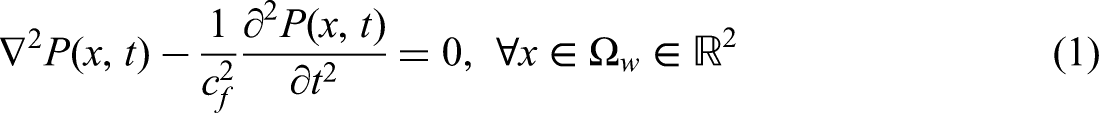
Sound pressure control differential equation

Consider a region ${\mathrm{\Omega }}_w$ , a boundary $\mathrm{\Gamma }:=\mathrm{\partial }{\mathrm{\Omega }}_w$ , a complement ${\mathrm{\Omega }}_{\mathrm{n}}:=\mathrm{U}\mathrm{\setminus }{\mathrm{\Omega }}_{\mathrm{w}}$ , and U representing the entire domain, as shown in Figure 1. When the domain is occupied by uniform ideal fluid, then the sound pressure satisfies the wave equation:

$${\mathrm{\nabla }}^{2}P(x,t)-{\displaystyle \frac{1}{c_f^2}{\displaystyle \frac{{\mathrm{\partial }}^{2}P(x,t)}{\mathrm{\partial }{t}^2}=0,\mathrm{\forall }x\in {\mathrm{\Omega }}_w\in {\mathbb{R}}^2}}$$

(1)

Figure 1.

Mathematical model of the acoustic field.

In the formula, ${\mathrm{\nabla }}^2$ denotes the Laplace operator, $P(x,t)$ represents the sound pressure at the midpoint x of the acoustic domain ${\mathrm{\Omega }}_w$ at time t, and $c_f$ is the wave velocity. In the case of a harmonic sound field, the sound pressure is given by:

$$\mathrm{p}(\mathrm{x},\mathrm{t})=\mathrm{p}(\mathrm{x}){\mathrm{e}}^{-\mathrm{i}\omega \mathrm{t}}$$

(2)

In the formula, $\mathrm{p}(\mathrm{x})$ represents the sound pressure value, the imaginary unit $\mathrm{i}=\sqrt{-1}$ , the angular frequency $\omega =2\pi \mathrm{f}$ , and ${\mathrm{e}}^{-\mathrm{i}wt}$ is the term varying with time.

Substituting equation (2) into equation (1) yields the Helmholtz control differential equation for the basic sound pressure:^51–53

$${\mathrm{\nabla }}^2\mathrm{p}(\mathrm{x})+{\mathrm{k}}^2\mathrm{p}(\mathrm{x})=0,\mathrm{\forall }\mathrm{x}\in {\mathrm{\Omega }}_{\mathrm{w}}$$

(3)

Boundary integral equations for acoustic scattering problems

By integrating the above Helmholtz equation and applying Green's second identity, the boundary integral equation for the sound field can be derived:

$$\mathrm{p}(\mathrm{x})+\underset{\mathrm{\Gamma }}{\int }{\displaystyle \frac{\mathrm{\partial }\mathrm{G}(\mathrm{x},\mathrm{y})}{\mathrm{\partial }\mathrm{n}(\mathrm{y})}\mathrm{p}(\mathrm{y})\mathrm{d}\mathrm{\Gamma }(\mathrm{y})=\underset{\mathrm{\Gamma }}{\int }\mathrm{G}(\mathrm{x},\mathrm{y})\mathrm{q}(\mathrm{y})\mathrm{d}\mathrm{\Gamma }(\mathrm{y})}$$

(4)

where $\mathrm{G}(\mathrm{x},\mathrm{y})$ is the Green's function, x is the source point, and y is the source point.

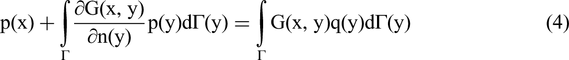
Considering the existence of non-uniform terms in the sound field ${\mathrm{\Omega }}_{\mathrm{w}}$ , that is, disturbances or sound sources, the field point x is approached to the integral boundary $\mathrm{\Gamma }$ , that is, $\mathrm{x}\in \mathrm{\Gamma }$ , then the conventional boundary integral equation considering the incident wave is expressed as

$$\mathrm{c}(\mathrm{x})\mathrm{p}(\mathrm{x})+\underset{\mathrm{\Gamma }}{\int }{\displaystyle \frac{\mathrm{\partial }\mathrm{G}(\mathrm{x},\mathrm{y})}{\mathrm{\partial }\mathrm{n}(\mathrm{y})}\mathrm{p}(\mathrm{y})\mathrm{d}\mathrm{\Gamma }(\mathrm{y})=\underset{\mathrm{\Gamma }}{\int }\mathrm{G}(\mathrm{x},\mathrm{y})\mathrm{q}(\mathrm{y})\mathrm{d}\mathrm{\Gamma }(\mathrm{y})+{\mathrm{p}}_{\mathrm{in}}(\mathrm{x}),\mathrm{x}\in \mathrm{\Gamma }}$$

(5)

${\mathrm{p}}_{\mathrm{in}}(\mathrm{x})$ represents the acoustic pressure of the incident wave at point x. The value of $\mathrm{c}(\mathrm{x})$ is determined by the boundary geometry at the source point x. If the boundary is smooth at point x., then $\mathrm{c}(\mathrm{x})=1/2$ .

Taking the derivative with respect to its external normal $\mathrm{n}(\mathrm{x})$ :

$$\mathrm{c}(\mathrm{x})\mathrm{q}(\mathrm{x})+\underset{\mathrm{\Gamma }}{\int }{\displaystyle \frac{{\mathrm{\partial }}^2\mathrm{G}(\mathrm{x},\mathrm{y})}{\mathrm{\partial }\mathrm{n}(\mathrm{x})\mathrm{\partial }\mathrm{n}(\mathrm{y})}\mathrm{p}(\mathrm{y})\mathrm{d}\mathrm{\Gamma }(\mathrm{y})=\underset{\mathrm{\Gamma }}{\int }{\displaystyle \frac{\mathrm{\partial }\mathrm{G}(\mathrm{x},\mathrm{y})}{\mathrm{\partial }\mathrm{n}(\mathrm{x})}\mathrm{q}(\mathrm{y})\mathrm{d}\mathrm{\Gamma }(\mathrm{y})+{\displaystyle \frac{\mathrm{\partial }{\mathrm{p}}_{\mathrm{in}}(\mathrm{x})}{\mathrm{\partial }\mathrm{n}(\mathrm{x})}}}}$$

(6)

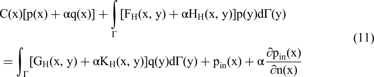
To avoid calculation instability at certain frequencies and the deviation from the correct solution when dealing with the external sound field problem, that is, the existence of false eigenfrequencies, the Burto–Miller method is used to obtain an accurate and unique solution.^54,55

$$\begin{array}{rl}& C(x)[p(x)+\alpha q(x)]+\underset{\mathrm{\Gamma }}{\int }[F(x,y)+\alpha H(x,y)]p(y)d\mathrm{\Gamma }(y)\\ & ={\int }_{\mathrm{\Gamma }}[G(x,y)+\alpha K(x,y)]q(y)d\mathrm{\Gamma }(y)+p_{in}(x)+\alpha {\displaystyle \frac{\mathrm{\partial }{p}_{in}(x)}{\mathrm{\partial }n(x)}}\end{array}$$

(7)

where $\alpha$ represents the coupling coefficient, if the wave number $\mathrm{k}\ge 1$ , then $\mathrm{a}=\mathrm{i}/\mathrm{k}$ ; otherwise $\mathrm{a}=\mathrm{i}$ . $\mathrm{F}(\mathrm{x},\mathrm{y})$ is the normal derivative of $\mathrm{G}(\mathrm{x},\mathrm{y})$ .

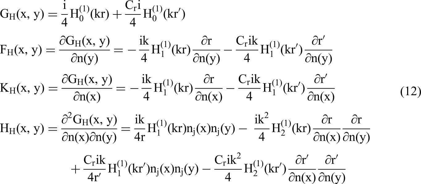
For the two-dimensional sound field problem, the kernel function is expressed as follows:^56,57

$$\begin{array}{rl}& G(x,y)={\displaystyle \frac{i}{4}{H}_0^{(1)}(kr)}\\ & F(x,y)={\displaystyle \frac{\mathrm{\partial }G(x,y)}{\mathrm{\partial }n(y)}=-{\displaystyle \frac{ik}{4}{H}_1^{(1)}(kr){\displaystyle \frac{\mathrm{\partial }r}{\mathrm{\partial }n(y)}}}}\\ & K(x,y)={\displaystyle \frac{\mathrm{\partial }G(x,y)}{\mathrm{\partial }n(x)}=-{\displaystyle \frac{ik}{4}{H}_1^{(1)}(kr){\displaystyle \frac{\mathrm{\partial }r}{\mathrm{\partial }n(x)}}}}\\ & H(x,y)={\displaystyle \frac{{\mathrm{\partial }}^{2}G(x,y)}{\mathrm{\partial }n(x)\mathrm{\partial }n(y)}={\displaystyle \frac{ik}{4}{H}_1^{(1)}(kr)n_j(x)n_j(y)-{\displaystyle \frac{i{k}^2}{4}{H}_2^{(1)}(kr){\displaystyle \frac{\mathrm{\partial }r}{\mathrm{\partial }n(x)}{\displaystyle \frac{\mathrm{\partial }r}{\mathrm{\partial }n(y)}}}}}}\end{array}$$

(8)

where, $\mathrm{r}=|\mathrm{x}-\mathrm{y}|$ , ${\mathrm{H}}_{\mathrm{n}}^{(1)}$ is the first-kind n-order Hankel function.

Ground reflection

When the model accounts for ground reflection, the ground is treated as an infinite rigid baffle, simplifying the sound field problem to a two-dimensional half-space problem. According to the mirror principle, the basic solution to the half-space sound field problem can be expressed as:

$$\begin{array}{rl}& G_H(x,y)=G(x,y)+C_{r}G(x^{\mathrm{\prime }},y)\\ & G_H(x,y)={\displaystyle \frac{i}{4}{H}_0^{(1)}(k|x-y|)+{\displaystyle \frac{i}{4}{H}_0^{(1)}(k|x^{\mathrm{\prime }}-y|)}}\end{array}$$

(9)

In the formula, ${\mathrm{x}}^{\mathrm{\prime }}$ is the mirror point of the field point x about the symmetry plane, ${\mathrm{C}}_{\mathrm{r}}$ is the reflection coefficient, if the symmetry plane is a total reflection plane, ${\mathrm{C}}_{\mathrm{r}}=1$ , if the symmetry plane is a total absorption plane, ${\mathrm{C}}_{\mathrm{r}}=0$ . If the reflection interface in the semi-free sound field is not completely rigid, such as in real situations, the ground is not a completely rigid wall, such as sand, sandy land covered with lawn, and ground with snow, then under the action of the incident wave, the interface will undergo a slight deformation.^58,59 At this time, part of the energy of the incident sound wave is absorbed by the interface, so that the phase and amplitude of the sound pressure will change after the sound wave is reflected by the ground, and the reflection effect is different for sound waves with different incident angles and different reflection interface properties. When the sound wave is incident obliquely on the material surface at a certain specific angle, that is, the incident angle is between 0 and 90 degrees, taking into full account the impedance effect of the reflection interface, assuming that the specific admittance of the reflection interface is uniform, the sound pressure reflection coefficient on the reflection interface can be approximately expressed as

$${\mathrm{C}}_{\mathrm{r}}={\displaystyle \frac{\cos \theta -\mathrm{T}}{\cos \theta +\mathrm{T}}}$$

(10)

where, $\theta$ is the incident angle and T is the specific admittance of the reflecting interface.

In a semi-free sound field, the actual sound pressure results from the combined effect of the direct sound pressure and the indirect radiation sound pressure reflected by the reflecting surface (as shown in Figure 2).

Figure 2.

The propagation of sound waves in a semi-free sound field.

Substituting equations (9) and (10) into (7), we can get the Burton–Miller integral equation of the sound field after considering the ground reflection using ${\mathrm{r}}^{\mathrm{\prime }}$ :

$$\begin{array}{rl}& C(x)[p(x)+\alpha q(x)]+\underset{\mathrm{\Gamma }}{\int }[F_H(x,y)+\alpha H_H(x,y)]p(y)d\mathrm{\Gamma }(y)\\ & ={\int }_{\mathrm{\Gamma }}[G_H(x,y)+\alpha K_H(x,y)]q(y)d\mathrm{\Gamma }(y)+p_{in}(x)+\alpha {\displaystyle \frac{\mathrm{\partial }{p}_{in}(x)}{\mathrm{\partial }n(x)}}\end{array}$$

(11)

in which

$$\begin{array}{rl}& G_H(x,y)={\displaystyle \frac{i}{4}{H}_0^{(1)}(kr)+{\displaystyle \frac{C_{r}i}{4}{H}_0^{(1)}(k{r}^{\mathrm{\prime }})}}\\ & F_H(x,y)={\displaystyle \frac{\mathrm{\partial }{G}_H(x,y)}{\mathrm{\partial }n(y)}=-{\displaystyle \frac{ik}{4}{H}_1^{(1)}(kr){\displaystyle \frac{\mathrm{\partial }r}{\mathrm{\partial }n(y)}-{\displaystyle \frac{C_{r}ik}{4}{H}_1^{(1)}(k{r}^{\mathrm{\prime }}){\displaystyle \frac{\mathrm{\partial }{r}^{\mathrm{\prime }}}{\mathrm{\partial }n(y)}}}}}}\\ & K_H(x,y)={\displaystyle \frac{\mathrm{\partial }{G}_H(x,y)}{\mathrm{\partial }n(x)}=-{\displaystyle \frac{ik}{4}{H}_1^{(1)}(kr){\displaystyle \frac{\mathrm{\partial }r}{\mathrm{\partial }n(x)}-{\displaystyle \frac{C_{r}ik}{4}{H}_1^{(1)}(k{r}^{\mathrm{\prime }}){\displaystyle \frac{\mathrm{\partial }{r}^{\mathrm{\prime }}}{\mathrm{\partial }n(x)}}}}}}\\ & H_H(x,y)={\displaystyle \frac{{\mathrm{\partial }}^2{G}_H(x,y)}{\mathrm{\partial }n(x)\mathrm{\partial }n(y)}={\displaystyle \frac{ik}{4r}{H}_1^{(1)}(kr)n_j(x)n_j(y)-{\displaystyle \frac{i{k}^2}{4}{H}_2^{(1)}(kr){\displaystyle \frac{\mathrm{\partial }r}{\mathrm{\partial }n(x)}{\displaystyle \frac{\mathrm{\partial }r}{\mathrm{\partial }n(y)}}}}}}\\ & +{\displaystyle \frac{C_{r}ik}{4r^{\mathrm{\prime }}}{H}_1^{(1)}(k{r}^{\mathrm{\prime }})n_j(x)n_j(y)-{\displaystyle \frac{C_{r}i{k}^2}{4}{H}_2^{(1)}(k{r}^{\mathrm{\prime }}){\displaystyle \frac{\mathrm{\partial }{r}^{\mathrm{\prime }}}{\mathrm{\partial }n(x)}{\displaystyle \frac{\mathrm{\partial }{r}^{\mathrm{\prime }}}{\mathrm{\partial }n(y)}}}}}\end{array}$$

(12)

NURBS-based isogeometric boundary element analysis

For two-dimensional boundary elements, IGABEM is employed to solve acoustic field problems.^60,61 Leveraging B-splines and Non-Uniform Rational B-Splines (NURBS) provide high-precision representations of curves and surfaces, enabling accurate modeling of intricate free-form geometries. IGA directly utilizes the NURBS control points of the geometric model as optimization variables, allowing for efficient and precise shape optimization based on the optimized control point coordinates and weights. The result is a smooth and continuous NURBS-based boundary. By incorporating rational functions, IGA enhances control over geometric representation, facilitating flexible local adjustments and seamless adaptation to a wide range of complex, irregular, and non-uniform geometries.

B-spline curves and NURBS

B-spline is an extension of the Bezier curve and can be seen as the splicing of many groups of Bezier curves. It has three main elements: knots, control points, and degree. Given a knot vector $\mathrm{U}=\{{\mathrm{u}}_0,{\mathrm{u}}_1,\cdots ,{\mathrm{u}}_{\mathrm{m}}{\}}^{\mathrm{\top }}$ , using the Cox-de Boor recursive formula, as the degree of the NURBS basis function p＞0, the higher-order basis functions in the B-spline basis function are expressed as:^62,63

$${\mathrm{N}}_{\mathrm{i},\mathrm{p}}(\mathrm{u})={\displaystyle \frac{\mathrm{u}-{\mathrm{u}}_{\mathrm{i}}}{{\mathrm{u}}_{\mathrm{i}+\mathrm{p}}-{\mathrm{u}}_{\mathrm{i}}}{\mathrm{N}}_{\mathrm{i},\mathrm{p}-1}(\mathrm{u})+{\displaystyle \frac{{\mathrm{u}}_{\mathrm{i}+\mathrm{p}+1}-\mathrm{u}}{{\mathrm{u}}_{\mathrm{i}+\mathrm{p}+1}-{\mathrm{u}}_{\mathrm{i}+1}}{\mathrm{N}}_{\mathrm{i}+1,\mathrm{p}-1}(\mathrm{u})}}$$

(13)

The k-th derivative of ${\mathrm{N}}_{\mathrm{i},\mathrm{p}}(\mathrm{u})$ can be presented as:

$${\displaystyle \frac{{\mathrm{d}}^{\mathrm{k}}}{\mathrm{d}{\mathrm{u}}^{\mathrm{k}}}{\mathrm{N}}_{\mathrm{i},\mathrm{p}}(\mathrm{u})={\displaystyle \frac{\mathrm{p}}{{\mathrm{u}}_{\mathrm{i}+\mathrm{p}}-{\mathrm{u}}_{\mathrm{i}}}\left({\displaystyle \frac{{\mathrm{d}}^{\mathrm{k}-1}}{\mathrm{d}{\mathrm{u}}^{\mathrm{k}-1}}{\mathrm{N}}_{\mathrm{i},\mathrm{p}-1}(\mathrm{u})}\right)-{\displaystyle \frac{\mathrm{p}}{{\mathrm{u}}_{\mathrm{i}+\mathrm{p}+1}-{\mathrm{u}}_{\mathrm{i}+1}}\left({\displaystyle \frac{{\mathrm{d}}^{\mathrm{k}-1}}{\mathrm{d}{\mathrm{u}}^{\mathrm{k}-1}}{\mathrm{N}}_{\mathrm{i}+1,\mathrm{p}-1}(\mathrm{u})}\right)(\mathrm{k}⩽\mathrm{p})}}}$$

(14)

By assigning a positive weight to each B-spline basis function, a NURBS basis function can be obtained. The p-degree NURBS basis function ${\mathrm{R}}_{\mathrm{i},\mathrm{p}}(\mathrm{u})$ can be expressed as:

$${\mathrm{R}}_{\mathrm{i},\mathrm{p}}(\mathrm{u})={\displaystyle \frac{{\mathrm{N}}_{\mathrm{i},\mathrm{p}}(\mathrm{u}){\mathrm{w}}_{\mathrm{i}}}{{\sum }_{\mathrm{i}=0}^{\mathrm{n}}{\mathrm{N}}_{\mathrm{i}.\mathrm{p}}(\mathrm{u}){\mathrm{w}}_{\mathrm{i}}}(\mathrm{i}=0,1,\dots ,\mathrm{n})}$$

(15)

where ${\mathrm{w}}_{\mathrm{i}}$ is the weight coefficient and n is the maximum index of the basis function.

The first-order derivative of the NURBS basis function can be stated as:

$${\displaystyle \frac{\mathrm{d}}{\mathrm{du}}{\mathrm{R}}_{\mathrm{i},\mathrm{p}}(\mathrm{u})={\mathrm{w}}_{\mathrm{i}}{\displaystyle \frac{{\sum }_{\mathrm{i}=0}^{\mathrm{n}}{\mathrm{N}}_{\mathrm{i}.\mathrm{p}}(\mathrm{u}){\mathrm{w}}_{\mathrm{i}}{\displaystyle \frac{\mathrm{d}}{\mathrm{du}}{\mathrm{N}}_{\mathrm{i},\mathrm{p}}(\mathrm{u})-{\mathrm{N}}_{\mathrm{i},\mathrm{p}}(\mathrm{u}){\sum }_{\mathrm{i}=0}^{\mathrm{n}}{\mathrm{w}}_{\mathrm{i}}{\displaystyle \frac{\mathrm{d}}{\mathrm{du}}{\mathrm{N}}_{\mathrm{i},\mathrm{p}}(\mathrm{u})}}}{{\left({\sum }_{\mathrm{i}=0}^{\mathrm{n}}{\mathrm{N}}_{\mathrm{i}.\mathrm{p}}(\mathrm{u}){\mathrm{w}}_{\mathrm{i}}\right)}^2}}}$$

(16)

With the NURBS basis function ${\mathrm{R}}_{\mathrm{i},\mathrm{p}}(\mathrm{u})$ , given a set of control points ${\mathrm{x}}_{\mathrm{i}}=0,1,\dots ,\mathrm{n}$ , the NURBS curve can be written as:

$$\mathrm{x}(\mathrm{u})=\sum _{\mathrm{i}=0}^{\mathrm{n}}{\mathrm{R}}_{\mathrm{i}.\mathrm{p}}(\mathrm{u}){\mathrm{x}}_{\mathrm{i}}$$

(17)

This article uses the above-mentioned NURBS basis functions to discretize the geometry and field variables in acoustic field boundary integral equations.

Isogeometric BEM

The discretization of the boundary curve is as shown in equation (17), and the sound pressure p and sound flux q on the boundary can be written as:^64–66

$$\begin{array}{rl}& p(u)=\sum _{i=0}^n{R}_{i,p}(u)P_i=R_p(u)P\\ & q(u)=\sum _{i=0}^n{R}_{i,p}(u)Q_i=R_p(u)Q\end{array}$$

(18)

Substituting equations (17), (18) into the boundary integral equation (11), we can obtain

$$\begin{array}{rl}& C(u_x)R_p(u_x)[P+\alpha Q]+\sum _{j=0}^{n-1}\left\{\underset{{(u_y)}_j}{\overset{{(u_y)}_{j+1}}{\int }}[F_H(u_x,u_y)+\alpha H_H(u_x,u_y)]R_p(u_y)P\right\}|J_{u_y}|d{u}_y\\ & =\sum _{j=0}^{n-1}\left\{\underset{{(u_y)}_j}{\overset{{(u_y)}_{j+1}}{\int }}[G_H(u_x,u_y)+\alpha K_H(u_x,u_y)]R_p(u_y)Q\right\}|J_{u_y}|d{u}_y+p_{in}(u_x)+\alpha {\displaystyle \frac{\mathrm{\partial }{p}_{in}(u_x)}{\mathrm{\partial }n(u_x)}}\end{array}$$

(19)

where the subscript j represents the number of control points.

In the traditional boundary element method, in order to simplify the solution process, the collocation points are usually selected on the nodes of the boundary element. However, after discretizing the boundary variables using NURBS, the generalized control points to be found are usually not located on the boundary. Therefore, the selection of collocation points is different from that of the traditional BEM. The collocation points are determined by calculating the Greville coordinates associated with the basis functions, ⁶⁷ the selection expression is:

$${\mathrm{u}}_0={\displaystyle \frac{{\mathrm{u}}_{\mathrm{i}+1}+{\mathrm{u}}_{\mathrm{i}+2}+\dots +{\mathrm{u}}_{\mathrm{i}+\mathrm{p}}}{\mathrm{p}}(\mathrm{i}=0,1,\dots ,\mathrm{n}-1)}$$

(20)

The point selection method shown in equation (20) avoids repeated selection of points at the beginning and end of the boundary curve. Figure 3 shows the NURBS curve defined by the node vector $\mathrm{U}=(0,0,0,0.25,0.25,0.5,0.5,0.75,0.75,1,1,1)$ , the corresponding control point locations, and the collocation point locations.

Figure 3.

NURBS curve with control points and collocation points.

We introduce coefficient matrices G and H, equation (19) can be rewritten in the following matrix form:

$$\mathrm{Hp}=\mathrm{Gq}+{\mathrm{p}}_{\mathrm{in}}$$

(21)

where H and G represent the coefficient matrices of the boundary element, while p and q correspond to the sound pressure and sound flux vectors on the boundary. Additionally, ${\mathrm{p}}_{\mathrm{in}}$ is the vector that represents the contribution of the incident wave.

In this article, an impedance boundary condition $\mathrm{q}(\mathrm{x})=\mathrm{i}\mathrm{k}\beta (\mathrm{x})\mathrm{P}(\mathrm{x})$ is introduced, which allows equation (21) to be rewritten as follows:

$$[\mathrm{H}-\mathrm{GB}]\mathrm{p}={\mathrm{p}}_{\mathrm{in}}$$

(22)

where

$$\mathrm{B}=\mathrm{ik}\left[\begin{array}{ccc}{\beta }_1& \dots & 0\\ \dots & \dots & \dots \\ 0& \dots & {\beta }_n\end{array}\right]$$

(23)

here, β _i denotes the normalized admittance corresponding to the ith element.

It can be inferred from equation (12) that the wave number k is present in the kernel function, causing equation (22) to be frequency dependent. This frequency dependence leads to high computational cost when solving broadband problems, as the coefficient matrix must be recalculated at each frequency point. To address this computational burden, this research applies Taylor series expansion to decouple the kernel function into components that are either dependent or independent of frequency, as described in the following procedure.

Taylor expansion form of the boundary integral equation of the acoustic field

At the fixed frequency expansion point k₀r, the first-order nth Hankel function in G(x, y), which depends on the wave number k, can be expressed as a Taylor series expansion:^68,69

$${\mathrm{H}}_{\mathrm{n}}^{(1)}(\mathrm{kr})=\sum _{\mathrm{m}=0}^{\mathrm{\infty }}{\displaystyle \frac{{(\mathrm{kr}-{\mathrm{k}}_0\mathrm{r})}^{\mathrm{m}}}{\mathrm{m}!}{\displaystyle \frac{{\mathrm{d}}^{\mathrm{m}}{\mathrm{H}}_{\mathrm{n}}^{(1)}(\mathrm{kr})}{\mathrm{d}{(\mathrm{kr})}^{\mathrm{m}}}{|}_{\mathrm{kr}={\mathrm{k}}_0\mathrm{r}}}}$$

(24)

m is the number of expansion items.

For the calculation of infinite Taylor series, we truncate it to finite terms to approximate the calculation. For example, we truncate the infinite series in the Taylor series expansion to the w-th term, expressed as:

$${\mathrm{T}}_{\mathrm{w}}^{(1)}(\mathrm{kr})=\sum _{\mathrm{m}=0}^{\mathrm{w}}{\displaystyle \frac{{(\mathrm{kr}-{\mathrm{k}}_0\mathrm{r})}^{\mathrm{m}}}{\mathrm{m}!}{\displaystyle \frac{{\mathrm{d}}^{\mathrm{m}}{\mathrm{H}}_{\mathrm{n}}^{(1)}(\mathrm{kr})}{\mathrm{d}{(\mathrm{kr})}^{\mathrm{m}}}{|}_{\mathrm{kr}={\mathrm{k}}_0\mathrm{r}}}}$$

(25)

This is the w-th-order approximation of the Taylor series expansion, also known as the Taylor polynomial. When w tends to infinity, ${\mathrm{T}}_{\mathrm{w}}^{(1)}(\mathrm{kr})$ will approach infinitely to ${\mathrm{H}}_{\mathrm{n}}^{(1)}(\mathrm{kr})$ . It is worth noting that tailor expansion is performed for the neighborhood of a point. This means it is only valid within a specific radius of convergence, diverging beyond this range, and generally, this range must be extremely small.

As the infinite terms of the Taylor series expansion cannot be computed, its error is assessed through truncation error. The truncation error is defined as:

$${\mathrm{R}}_{\mathrm{w}}^{(1)}(\mathrm{kr})={\mathrm{H}}_{\mathrm{n}}^{(1)}(\mathrm{kr})-{\mathrm{T}}_{\mathrm{w}}^{(1)}(\mathrm{kr})$$

(26)

The truncation error represents the difference between the Taylor polynomial and the function ${\mathrm{H}}_{\mathrm{n}}^{(1)}(\mathrm{kr})$ , that is, the size of the error when we use the Taylor polynomial to approximate represent ${\mathrm{H}}_{\mathrm{n}}^{(1)}(\mathrm{kr})$ . When the larger the w, the smaller the error of the Taylor polynomial, but the computational workload is also larger. Therefore, we need to evaluate the choice of w.

When evaluating the error, we can use the Lagrange remainder theorem to express the truncation error in the form of a remainder, that is, we need to use the remainder of Taylor's formula for evaluation. It is defined as:

$${\mathrm{R}}_{\mathrm{w}}^{(1)}(\mathrm{kr})={\displaystyle \frac{{(\mathrm{kr}-{\mathrm{k}}_0\mathrm{r})}^{\mathrm{w}+1}}{(\mathrm{w}+1)!}{\displaystyle \frac{{\mathrm{d}}^{(\mathrm{w}+1)}{\mathrm{H}}_{\mathrm{n}}^{(1)}(\phi )}{\mathrm{d}{(\mathrm{kr})}^{\mathrm{w}+1}}}}$$

(27)

here $\phi$ is a number between kr and k₀r. This remainder represents the size of the truncation error when using the wth Taylor polynomial of order to approximate represent ${\mathrm{H}}_{\mathrm{n}}^{(1)}(\mathrm{kr})$ . Usually, we hope that the truncation error is smaller than a preset error bound, that is: ⁷⁰

$$|{\mathrm{R}}_{\mathrm{w}}^{(1)}(\mathrm{kr})|\le ϵ$$

(28)

$ϵ$ represents a user-defined tolerance that can determine the value of w.

For the Hankel function involving wave number, when the fixed expansion point is set at the midpoint of the frequency range, if it does not satisfy equation (28), the frequency range will be automatically split into two sub-ranges, where a similar Taylor expansion is applied to each sub-range. This procedure continues iteratively until all frequency sub-ranges satisfy equation (28) (see Figure 4).

Figure 4.

Frequency division method in Taylor expansion terms.

Substituting equation (24) into equation (11), the integral form at the fixed frequency expansion point k₀ is obtained ⁷¹ :

$$\begin{array}{rl}& \underset{\mathrm{\Gamma }}{\int }{G}_H(x,y)q(y)d\mathrm{\Gamma }(y)=\sum _{m=0}^{\mathrm{\infty }}{\displaystyle \frac{{(k-k_0)}^m}{m!}({kI}_{g1}^m+{kI}_{g2}^m)}\\ & \underset{\mathrm{\Gamma }}{\int }{F}_H(x,y)p(y)d\mathrm{\Gamma }(y)=\sum _{m=0}^{\mathrm{\infty }}{\displaystyle \frac{{(k-k_0)}^m}{m!}(I_{f1}^m+I_{f2}^m)}\\ & \alpha \underset{\mathrm{\Gamma }}{\int }{K}_H(x,y)q(y)d\mathrm{\Gamma }(y)=\sum _{m=0}^{\mathrm{\infty }}{\displaystyle \frac{{(k-k_0)}^m}{m!}(k^2{I}_{k1}^m+k^2{I}_{k2}^m)}\\ & \alpha \underset{\mathrm{\Gamma }}{\int }{K}_H(x,y)p(y)d\mathrm{\Gamma }(y)=\sum _{m=0}^{\mathrm{\infty }}{\displaystyle \frac{{(k-k_0)}^m}{m!}({kI}_{h1}^m-k^2{I}_{h2}^m+{kI}_{h3}^m-k^2{I}_{h4}^m)}\end{array}$$

(29)

where

$$\begin{array}{rl}& I_{g1}^m=-\underset{\mathrm{\Gamma }}{\int }{\displaystyle \frac{{\beta }_i{r}^m}{4}{\displaystyle \frac{d^m{H}_0^{(1)}(kr)}{d{(kr)}^m}{|}_{kr=k_{0}r}p(y)d\mathrm{\Gamma }(y)}}\\ & I_{g2}^m=-\underset{\mathrm{\Gamma }}{\int }{\displaystyle \frac{C_r{\beta }_i{(r^{\mathrm{\prime }})}^m}{4}{\displaystyle \frac{d^m{H}_0^{(1)}(k{r}^{\mathrm{\prime }})}{d{(k{r}^{\mathrm{\prime }})}^m}{|}_{k{r}^{\mathrm{\prime }}=k_0{r}^{\mathrm{\prime }}}p(y)d\mathrm{\Gamma }(y)}}\\ & I_{f1}^m=-\underset{\mathrm{\Gamma }}{\int }{\displaystyle \frac{i{r}^{m}k}{4}{\displaystyle \frac{d^m{H}_1^{(1)}(kr)}{d{(kr)}^m}{|}_{kr=k_{0}r}{\displaystyle \frac{\mathrm{\partial }r}{\mathrm{\partial }n(y)}p(y)d\mathrm{\Gamma }(y)}}}\\ & I_{f2}^m=-\underset{\mathrm{\Gamma }}{\int }{\displaystyle \frac{C_{r}i{(r^{\mathrm{\prime }})}^{m}k}{4}{\displaystyle \frac{d^m{H}_1^{(1)}(k{r}^{\mathrm{\prime }})}{d{(k{r}^{\mathrm{\prime }})}^m}{|}_{k{r}^{\mathrm{\prime }}=k_0{r}^{\mathrm{\prime }}}{\displaystyle \frac{\mathrm{\partial }{r}^{\mathrm{\prime }}}{\mathrm{\partial }n(y)}p(y)d\mathrm{\Gamma }(y)}}}\\ & I_{k1}^m=\underset{\mathrm{\Gamma }}{\int }{\displaystyle \frac{\alpha {\beta }_i{r}^m}{4}{\displaystyle \frac{d^m{H}_1^{(1)}(kr)}{d{(kr)}^m}{|}_{kr=k_{0}r}{\displaystyle \frac{\mathrm{\partial }r}{\mathrm{\partial }n(x)}p(y)d\mathrm{\Gamma }(y)}}}\\ & I_{k2}^m=\underset{S}{\int }{\displaystyle \frac{\alpha C_r{\beta }_i{(r^{\mathrm{\prime }})}^m}{4}{\displaystyle \frac{d^m{H}_1^{(1)}(k{r}^{\mathrm{\prime }})}{d{(k{r}^{\mathrm{\prime }})}^m}{|}_{k{r}^{\mathrm{\prime }}=k_0{r}^{\mathrm{\prime }}}{\displaystyle \frac{\mathrm{\partial }{r}^{\mathrm{\prime }}}{\mathrm{\partial }n(x)}p(y)d\mathrm{\Gamma }(y)}}}\end{array}$$

$$\begin{array}{rl}& I_{h1}^m=\underset{\mathrm{\Gamma }}{\int }{\displaystyle \frac{\alpha i{r}^{m-1}}{4}{\displaystyle \frac{d^m{H}_1^{(1)}(kr)}{d{(kr)}^m}{|}_{kr=k_{0}r}{n}_j(x)n_j(y)p(y)d\mathrm{\Gamma }(y)}}\\ & I_{h2}^m=\underset{\mathrm{\Gamma }}{\int }{\displaystyle \frac{\alpha i{r}^m}{4}{\displaystyle \frac{d^m{H}_2^{(1)}(kr)}{d{(kr)}^m}{|}_{kr=k_{0}r}{\displaystyle \frac{\mathrm{\partial }r}{\mathrm{\partial }n(x)}{\displaystyle \frac{\mathrm{\partial }r}{\mathrm{\partial }n(y)}p(y)d\mathrm{\Gamma }(y)}}}}\\ & I_{h3}^m=\underset{\mathrm{\Gamma }}{\int }{\displaystyle \frac{\alpha C_{r}i{(r^{\mathrm{\prime }})}^{m-1}}{4}{\displaystyle \frac{d^m{H}_1^{(1)}(k{r}^{\mathrm{\prime }})}{d{(k{r}^{\mathrm{\prime }})}^m}{|}_{k{r}^{\mathrm{\prime }}=k_0{r}^{\mathrm{\prime }}}{n}_j(x)n_j(y)p(y)d\mathrm{\Gamma }(y)}}\\ & I_{h4}^m=\underset{\mathrm{\Gamma }}{\int }{\displaystyle \frac{\alpha C_{r}i{(r^{\mathrm{\prime }})}^m}{4}{\displaystyle \frac{d^m{H}_2^{(1)}(k{r}^{\mathrm{\prime }})}{d{(k{r}^{\mathrm{\prime }})}^m}{|}_{k{r}^{\mathrm{\prime }}=k_0{r}^{\mathrm{\prime }}}{\displaystyle \frac{\mathrm{\partial }{r}^{\mathrm{\prime }}}{\mathrm{\partial }n(x)}{\displaystyle \frac{\mathrm{\partial }{r}^{\mathrm{\prime }}}{\mathrm{\partial }n(y)}p(y)d\mathrm{\Gamma }(y)}}}}\end{array}$$

(30)

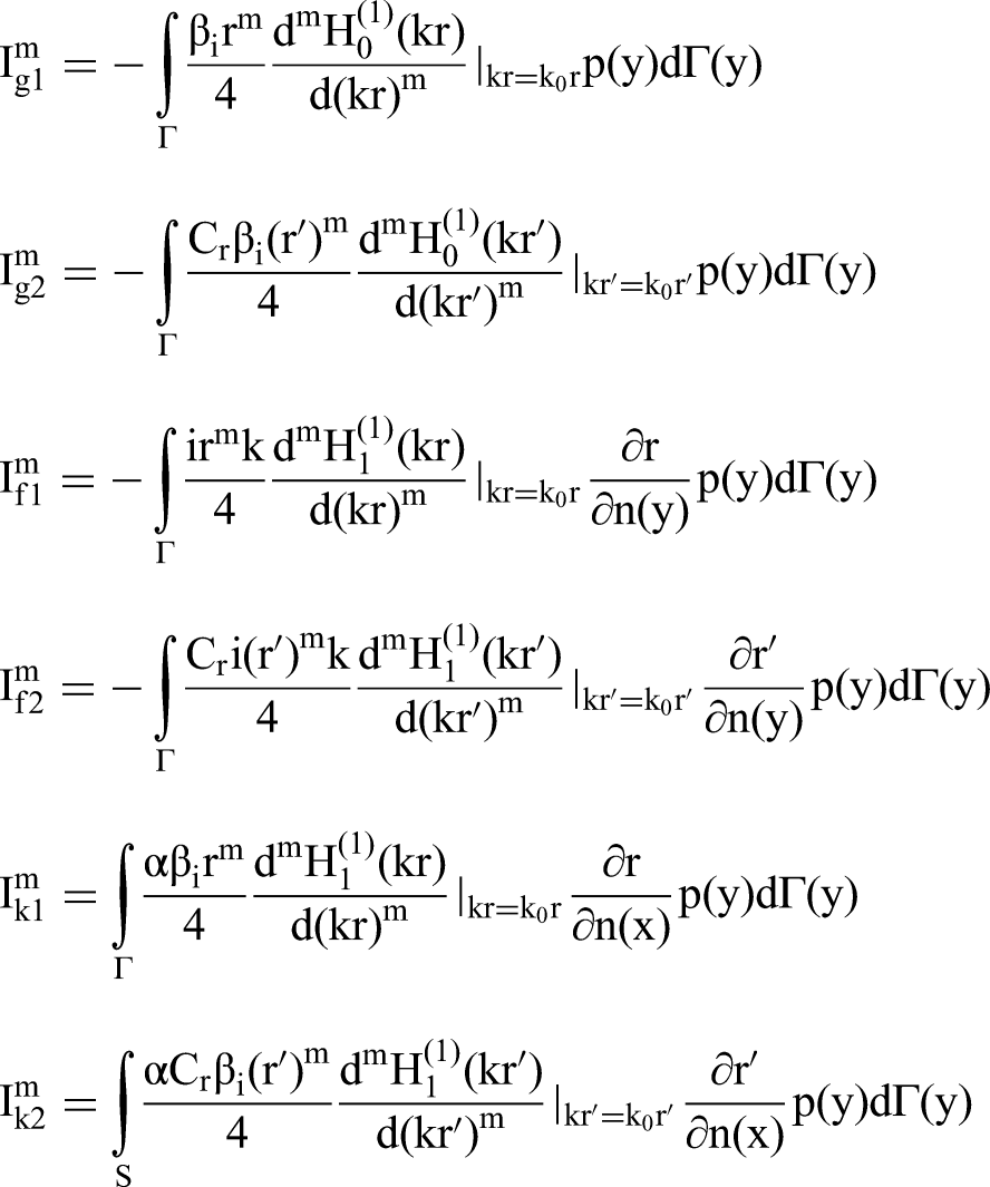
Substituting equation (30) into equation (11), we obtain:

$$\begin{array}{rl}& C(x)[p(x)(1+\alpha ik\beta (x))]+\sum _{m=0}^{\mathrm{\infty }}{\displaystyle \frac{{(k-k_0)}^m}{m!}[(I_{f1}^m+I_{f2}^m)+({kI}_{h1}^m+{kI}_{h3}^m-{kI}_{g1}^m-{kI}_{g2}^m)}\\ & -(k^2{I}_{h2}^m+k^2{I}_{h4}^m+k^2{I}_{k1}^m+k^2{I}_{k2}^m)]=p_{in}(x)+\alpha {\displaystyle \frac{\mathrm{\partial }{p}_{in}(x)}{\mathrm{\partial }n(x)}}\end{array}$$

(31)

A plane wave of unit amplitude traveling along the axis $\sigma$ is taken into consideration, then the incident sound pressure corresponding to the plane wave and its Taylor series expansion are as follows:

$${\mathrm{p}}_{\mathrm{in}}(\mathrm{x})={\mathrm{e}}^{\mathrm{ik}{\mathrm{x}}_{\sigma }}={\mathrm{e}}^{\mathrm{i}{\mathrm{k}}_0{\mathrm{x}}_{\sigma }}\sum _{\mathrm{m}=0}^{\mathrm{\infty }}{\displaystyle \frac{{[\mathrm{i}{\mathrm{x}}_{\sigma }(\mathrm{k}-{\mathrm{k}}_0)]}^{\mathrm{m}}}{\mathrm{m}!}}$$

(32)

where ${\mathrm{x}}_{\sigma }$ represents the $\sigma$ -axis coordinate of the source point, where $\sigma$ =x or y.

Substituting the above formula into equation (31), we get

$$\begin{array}{rl}& C(x)[p(x)(1+\alpha ik\beta (x))]+\sum _{m=0}^{\mathrm{\infty }}{\displaystyle \frac{{(k-k_0)}^m}{m!}[(I_{f1}^m+I_{f2}^m)+({kI}_{h1}^m+{kI}_{h3}^m-{kI}_{g1}^m-{kI}_{g2}^m)}\\ & -(k^2{I}_{h2}^m+k^2{I}_{h4}^m+k^2{I}_{k1}^m+k^2{I}_{k2}^m)]=e^{i{k}_0{x}_{\sigma }}\sum _{m=0}^{\mathrm{\infty }}{\displaystyle \frac{{({\mathrm{ix}}_{\sigma })}^m{(k-k_0)}^m}{m!}\left(1+\alpha ik{\displaystyle \frac{\mathrm{\partial }{x}_{\sigma }}{\mathrm{\partial }n(x)}}\right)}\end{array}$$

(33)

Applying the collocation method and constant elements to discretizing equation (33), we obtain:

$$\mathrm{Cp}+\mathrm{k}\overline{\mathrm{C}}\mathrm{p}+\sum _{\mathrm{m}=0}^{\mathrm{\infty }}{\displaystyle \frac{{(\mathrm{k}-{\mathrm{k}}_0)}^{\mathrm{m}}}{\mathrm{m}!}[{\mathrm{I}}_1^{\mathrm{m}}+{\mathrm{kI}}_2^{\mathrm{m}}+{\mathrm{k}}^2{\mathrm{I}}_3^{\mathrm{m}}]\mathrm{p}={\mathrm{P}}_{\mathrm{in}}}$$

(34)

where

$$\mathrm{C}=\left[\begin{array}{ccc}{\mathrm{C}}_1& \dots & 0\\ \dots & \dots & \dots \\ \dots & \dots & \dots \\ 0& \dots & {\mathrm{C}}_{\mathrm{N}}\end{array}\right]\mathrm{and}\overline{\mathrm{C}}=\alpha \mathrm{i}\left[\begin{array}{ccc}{\beta }_1{\mathrm{C}}_1& \dots & 0\\ \dots & \dots & \dots \\ \dots & \dots & \dots \\ 0& \dots & {\beta }_{\mathrm{N}}{\mathrm{C}}_{\mathrm{N}}\end{array}\right]$$

(35)

Define the matrices ${\overline{\mathrm{I}}}_1^{\mathrm{m}}$ and ${\overline{\mathrm{I}}}_2^{\mathrm{m}}$ as:

$${\overline{\mathrm{I}}}_1^{\mathrm{m}}=\{\begin{array}{ccc}\mathrm{C}+{\mathrm{I}}_1^{\mathrm{m}},& \mathrm{m}=0& \\ {\mathrm{I}}_1^{\mathrm{m}},& \mathrm{m}\ne 0& ,\end{array}{\overline{\mathrm{I}}}_2^{\mathrm{m}}=\{\begin{array}{ccc}\overline{\mathrm{C}}+{\mathrm{I}}_2^{\mathrm{m}},& \mathrm{m}=0& \\ {\mathrm{I}}_2^{\mathrm{m}},& \mathrm{m}\ne 0& \end{array}\mathrm{and}{\overline{\mathrm{I}}}_3^{\mathrm{m}}={\overline{\mathrm{I}}}_3^{\mathrm{m}}$$

(36)

Substituting into equation (34) we finally get:

$$\left[\sum _{\mathrm{m}=0}^{\mathrm{W}}{\displaystyle \frac{{(\mathrm{k}-{\mathrm{k}}_0)}^{\mathrm{m}}}{\mathrm{m}!}({\overline{\mathrm{I}}}_1^{\mathrm{m}}+\mathrm{k}{\overline{\mathrm{I}}}_2^{\mathrm{m}}+{\mathrm{k}}^2{\overline{\mathrm{I}}}_3^{\mathrm{m}})}\right]\mathrm{p}={\overline{\mathrm{P}}}_{\mathrm{in}},$$

(37)

The Taylor expansion is truncated to retain only the first W terms. The coefficient matrices ${\overline{\mathrm{I}}}_1^m$ , ${\overline{\mathrm{I}}}_2^m$ , and ${\overline{\mathrm{I}}}_3^m$ are independent of frequency. Therefore, it only needs to be calculated once in a multi-frequency acoustic analysis, which takes low computational cost without repeatedly solving the frequency-dependent equation (24). However, although BEM reduces the computational dimension, the coefficient matrix is dense, with high memory and computational requirements. ⁷² In order to speed up the computation, deep neural network technology is used.

Application of neural networks in acoustic computing

A neural network is a computational framework that mimics the connection pattern of neurons in the human brain, comprising an input layer, one or more hidden layers, and an output layer.^73–75 The input layer of a neural network receives input data; the hidden layer is composed of multiple layers of neurons, which are mainly used for feature extraction and pattern learning; the output layer is the result of output prediction. Each “neuron” is a basic computing unit used to process input signals and generate outputs. Deep neural networks usually have more hidden layers and can learn more complex feature representations. ⁷⁶ Since the computational complexity of neural network technology is mainly determined by the number of hidden layers and neurons, rather than the dimension of the input data, it only needs to adjust the number of neurons in the input layer to adapt to data of different dimensions. Therefore, the DNN model is selected for this data analysis task. We have obtained a large amount of high-quality training data through the simulation results of Taylor expansion of isogeometric boundary elements, trained multiple deep neural networks to build a reliable DNN model, and then predicted the sound pressure response of vibroacoustic problems across different parameter configurations and dimensional variations. The analysis process based on DNN is shown in Figure 5.

Figure 5.

Analysis process based on DNN.

Data set preparation: Select N values between [ ${\mathrm{x}}_{\min }$ , ${\mathrm{x}}_{\max }$ ] on the boundary $\mathrm{\Gamma }$ as samples X,^77–79 i.e.,

$$\mathrm{X}=\{{\mathrm{x}}^{\ell }|{\mathrm{x}}^{\ell }\in \mathcal{X},\ell =1,\dots ,\mathrm{N}\}$$

(38)

where x is $[{\mathrm{x}}_1,\cdots ,{\mathrm{x}}_{\mathrm{n}}{]}^{\mathrm{T}}$ . Using IGA FEM/BEM, the response Y at each point x is $[{\mathrm{y}}_1,\cdots ,{\mathrm{y}}_{\mathrm{n}}{]}^{\mathrm{T}}$ and can be calculated as follows:

$$\mathrm{Y}=\{{\mathrm{y}}^{\ell }|{\mathrm{y}}^{\ell }=\mathrm{f}({\mathrm{x}}^{\ell }),\ell =1,\dots ,\mathrm{N}\}$$

(39)

Assembling X and Y to get the dataset as follows:

$$\mathrm{Dataset}=\{({\mathrm{x}}^{\ell },{\mathrm{y}}^{\ell })|\ell =1,\dots ,\mathrm{N}\}$$

(40)

Use statistics to standardize the data set $({\mathrm{x}}^{\ell },{\mathrm{y}}^{\ell })$ . The main purpose of standardization is to convert feature data of different magnitudes into data of the uniform scale, thereby effectively removing differences in magnitude between them. Features of different magnitudes will have different degrees of impact on the model training process. Nonstandard data may cause the model to pay more attention to features with larger magnitudes and ignore features with smaller magnitudes. This will bias the training results of the model. Therefore, standardizing the model improves its generalization capability. The standardization process can be completed using the following formula:

$${\mathrm{S}}_{\mathrm{i}}^{\ell }={\displaystyle \frac{{\mathrm{z}}_{\mathrm{i}}^{\ell }-\mu }{\sigma }}$$

(41)

where ${\mathrm{S}}_{\mathrm{i}}^{\ell }$ denotes the standardized data, ${\mathrm{z}}_{\mathrm{i}}^{\ell }$ denotes the input/output of $({\mathrm{x}}^{\ell },{\mathrm{y}}^{\ell })$ , $\mu$ denotes the mean of the input/output, and $\sigma$ denotes the standard deviation of the input/output. The final standardized dataset is

$$\{({\mathrm{S}}_{{\mathrm{X}}^1},{\mathrm{S}}_{{\mathrm{y}}^1}),\dots ,({\mathrm{S}}_{{\mathrm{X}}^{\ell }},{\mathrm{S}}_{{\mathrm{y}}^{\ell }}),\dots ({\mathrm{S}}_{{\mathrm{X}}^{\mathrm{N}}},{\mathrm{S}}_{{\mathrm{y}}^{\mathrm{N}}})\}$$

(42)

After normalization, all features in the dataset are adjusted to a consistent scale. This adjustment ensures that the magnitude differences between various features do not affect the model training and prediction process.

Training and testing: To train and assess the model, the dataset in equation (42) is split into two subsets. ⁸⁰ The training data is used to create the mapping function f. This feature enables DNN to analyze multiple kinds and amounts of inputs and forecast matching outputs of varied kinds and sizes.

The DNN model is based on the principle of linear regression to adapt to the mapping relationship between input and output data. By using the information in the problem solution and input data to learn the mapping function, the forward calculation of DNN realizes linear and nonlinear transformations through a combination of linear layers and nonlinear activation functions. The calculation process of each layer can be described using the following equation:

$${\mathrm{h}}^0=\mathrm{x}\in {\mathbb{R}}^{{\mathrm{t}}_0}$$

$${\mathrm{h}}^{\mathrm{n}}=\mathrm{f}({\mathrm{W}}^{\mathrm{n}}{\mathrm{h}}^{(\mathrm{n}-1)}+{\mathrm{b}}^{\mathrm{n}})\in {\mathbb{R}}^{({\mathrm{t}}_{\mathrm{n}})}(1\le \mathrm{n}\le \mathrm{m})$$

$$\mathrm{z}=\mathrm{f}({\mathrm{W}}^{\mathrm{m}+1}{\mathrm{h}}^{\mathrm{m}}+{\mathrm{b}}^{\mathrm{m}+1})\in {\mathbb{R}}^{{\mathrm{t}}_{\mathrm{m}+1}}$$

(43)

Among them, ${\mathrm{h}}^0$ , ${\mathrm{h}}^{\mathrm{n}}$ , and $\mathrm{z}$ represent the values of the input layer, hidden layer, and output layer, respectively. ${\mathrm{t}}_0$ , ${\mathrm{t}}_{\mathrm{n}}$ , and ${\mathrm{t}}_{\mathrm{m}+1}$ represent the number of neurons in the input layer, the nth hidden layer, and the output layer, respectively. m and f represent the number of hidden layers and the activation function, respectively. ${\mathrm{W}}^{\mathrm{n}}\in {\mathbb{R}}^{{\mathrm{t}}_{\mathrm{n}}\times {\mathrm{t}}_{\mathrm{n}-1}}$ is the weight matrix, and ${\mathrm{b}}^{\mathrm{n}}\in {\mathbb{R}}^{{\mathrm{t}}_{\mathrm{n}}}$ is a bias vector of the linear transformation between layers.

Select a suitable learning rate to determine the optimal weights W and biases b. We chose Tanh, a widely used activation function in deep neural networks, to build our model.

Assume that the initial dataset with N samples is the training dataset, where ${\mathrm{X}}^{\ell }=({\mathrm{x}}_1^{\ell },{\mathrm{x}}_2^{\ell },\dots ,{\mathrm{x}}_{\mathrm{n}}^{\ell }{)}^{\mathrm{T}}$ is the input data and ${\mathrm{Y}}^{\ell }=({\mathrm{y}}_1^{\ell },{\mathrm{y}}_2^{\ell },\dots ,{\mathrm{y}}_{\mathrm{m}}^{\ell }{)}^{\mathrm{T}}$ is the actual value (target) that needs to be compared with the prediction (output). To obtain the best mapping function f and enhance the predictive ability of the model, the initial DNN model requires training, which is typically directed by a loss function. Predicting the response through DNN is a regression process. We use a loss function to evaluate the prediction accuracy after each forward propagation. The mean square error (MSE) is a typical loss function for this process because it effectively quantifies the difference between the model's predicted value and the actual value. Assuming the prediction is ${\mathrm{y}}_{\mathrm{pred},\mathrm{i}}$ (i represents the i-th unit), the MSE is as follows:

$$\mathrm{Loss}={\displaystyle \frac{1}{\mathrm{n}}\sum _{\mathrm{i}=1}^{\mathrm{n}}({\mathrm{y}}_{\mathrm{pred},\mathrm{i}}-{\mathrm{y}}_{\mathrm{true},\mathrm{i}}{)}^2}$$

(44)

where n is the number of test points. ${\mathrm{y}}_{\mathrm{pred},\mathrm{i}}$ and ${\mathrm{y}}_{\mathrm{true},\mathrm{i}}$ are the predicted value and the actual value, respectively.

It is challenging to thoroughly assess a DNN model's performance from every perspective using a single assessment metric. Therefore, additional metrics such as MAE (mean absolute error), symmetric mean absolute percentage error (SMAPE), and R-squared (R²) are introduced to evaluate the performance of the training model. The formulas for these metrics are as follows:

$$\mathrm{MAE}={\displaystyle \frac{1}{\mathrm{n}}\sum _{\mathrm{i}=1}^{\mathrm{n}}|{\mathrm{y}}_{\mathrm{pred},\mathrm{i}}-{\mathrm{y}}_{\mathrm{ture},\mathrm{i}}|}$$

(45)

$$\mathrm{SMAPE}={\displaystyle \frac{1}{\mathrm{n}}\sum _{\mathrm{i}=1}^{\mathrm{n}}{\displaystyle \frac{2|{\mathrm{y}}_{\mathrm{pred},\mathrm{i}}-{\mathrm{y}}_{\mathrm{true},\mathrm{i}}|}{|{\mathrm{y}}_{\mathrm{pred},\mathrm{i}}|+|{\mathrm{y}}_{\mathrm{true},\mathrm{i}}|}\times 100\text{\%}}}$$

(46)

$${\mathrm{R}}^2=1-{\displaystyle \frac{{\sum }_{\mathrm{i}=1}^{\mathrm{n}}{({\mathrm{y}}_{\mathrm{pred},\mathrm{i}}-{\mathrm{y}}_{\mathrm{true},\mathrm{i}})}^2}{{\sum }_{\mathrm{i}=1}^{\mathrm{n}}{(\overline{\mathrm{y}}-{\mathrm{y}}_{\mathrm{true},\mathrm{i}})}^2}}$$

(47)

and $\overline{\mathrm{y}}$ represents the mean of the true value.

The range of the three standards of MSE, MAE, and SMAPE is [0, +∞). When the predicted values are exactly the same as the true values, these values of standards are equal to 0, that is, a perfect model; the larger the error, the larger these values are, and the worse the model is. The advantage of MAE is that it clearly shows the difference between the model's predicted and actual values, effectively indicating the extent of deviation in predictions. R² is also called the coefficient of determination. Its value range is [0, 1], which reflects the accuracy of the model fitting the data. The closer the R² value is to 1, the better the model. These indicators do not have a fixed standard to judge the quality of the model. It needs to be judged in combination with the actual situation of the target variable (that is, the data to be predicted).

In addition, in order to minimize the loss value and improve the prediction accuracy of the model, it is necessary to continuously update the model parameters. This is achieved by using the back-propagation algorithm, which adjusts the parameters by calculating the gradient of the loss function with respect to the model parameters. In order to achieve efficient back-propagation, we use the optimization algorithm stochastic gradient descent (SGD) in this study to build an effective DNN model.

The trained model is then evaluated using the test dataset. Finally, post-processing for ${\mathrm{y}}_{\mathrm{pred},\mathrm{i}}$ is performed as follows:

$${\mathrm{y}}_{\mathrm{post},\mathrm{i}}={\mathrm{y}}_{\mathrm{pred},\mathrm{i}}\times \sigma +\mu$$

(48)

where ${\mathrm{y}}_{\mathrm{post},\mathrm{i}}$ represents the i-th post-processed value. Therefore, ${\mathrm{y}}_{\mathrm{post},\mathrm{i}}$ and ${\mathrm{y}}_{\mathrm{true},\mathrm{i}}$ can be used to calculate the accuracy of the model to judge the training effect of the DNN model.

After training, the best model we selected can predict the response of sound pressure using existing acoustic numerical simulation results as input.

Acoustic numerical examples

Studies have shown that the top structure of the sound barrier has a significant effect on improving the noise reduction effect of the sound barrier. The design of the top arc sound barrier can block the transmission of direct sound, isolate the transmitted sound, and attenuate the reflected sound. ⁸¹ In addition to these characteristics, the design of the top arc sound barrier makes installation more convenient and quick, and it can also be quickly disassembled and moved as needed, which is convenient for maintenance and management. Therefore, this article refers to the sound barrier structure of the highway and mainly simulates the top arc, cylindrical, and trapezoidal sound barriers.

This study uses Fortran 90 language and is numerically implemented by a desktop computer equipped with Intel (R) Core (TM) i7-8700 CPU and 16 GB RAM. To validate the effectiveness and applicability of the proposed algorithm, simulations are conducted for the three sound barrier examples presented in sections “Sound scattering of top curved sound barrier,” “Sound scattering of cylindrical sound barriers,” and “Sound scattering of trapezoidal sound barriers.” The sound pressure value of the model is calculated using Visual Studio 2013 software, and the sound pressure value is accelerated using the DNN acceleration model compiled in Python 3.9.

Sound scattering of top curved sound barrier

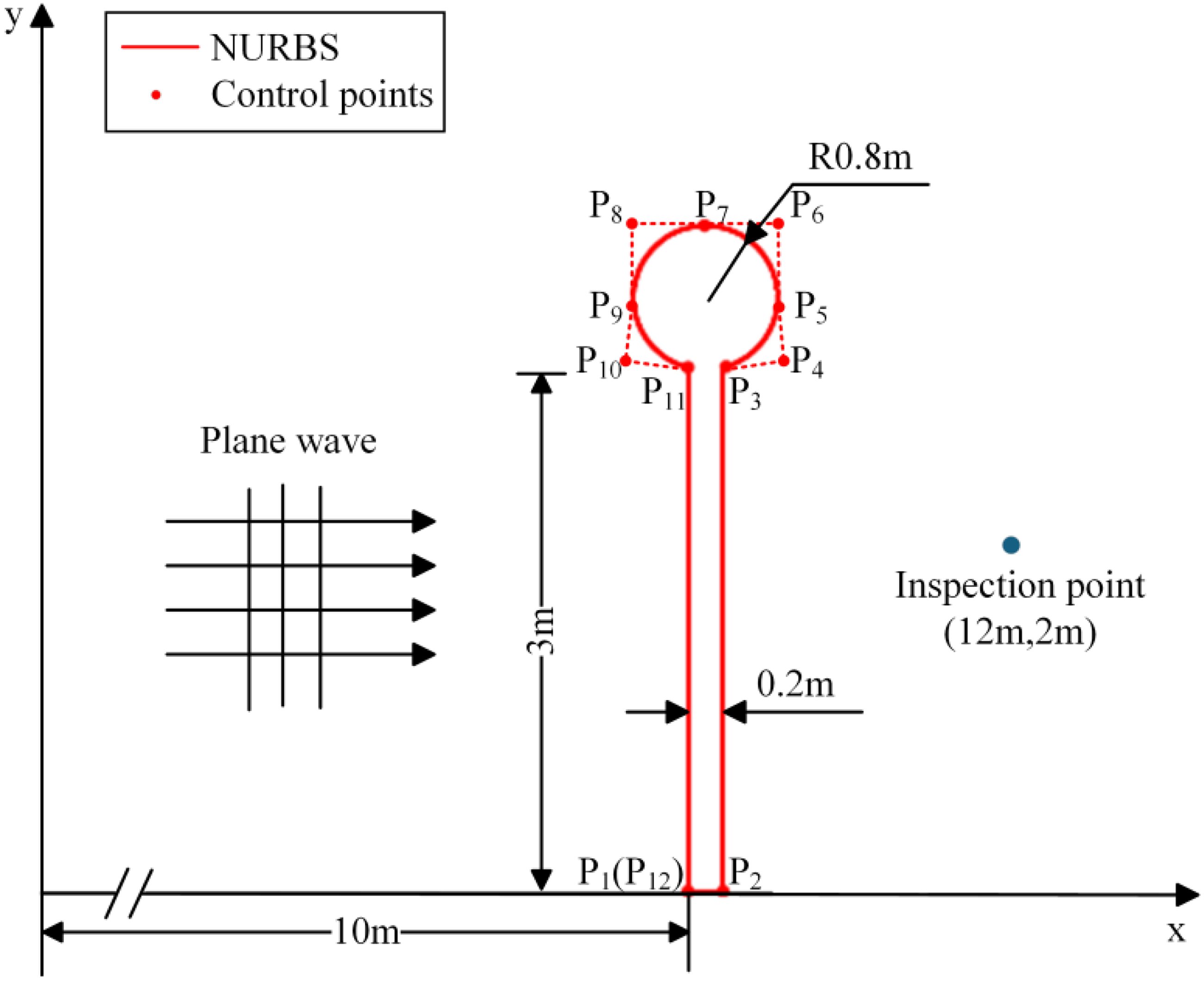
The algorithm proposed in this study was used to numerically simulate the scattered sound field of the semi-arc sound barrier under ground reflection conditions. The sound barrier model was constructed using an isogeometric model, generated by nine control points, and had a thickness of 0.2 m, then discretizing it with 831 constant boundary elements for calculation. The x-axis was set to a rigid ground, and a plane wave ${\mathrm{p}}_{\mathrm{in}}={\mathrm{p}}_0{\mathrm{e}}^{\mathrm{ikrcos}\theta }$ with an amplitude of p₀ = 1 was incident parallel to the ground along the positive direction of the x-axis. The model can be simplified to a 2D sound scattering problem in Figure 6. Make the inspection point located at (12 m, 2 m), and additional numerical simulation parameters are listed in Table 1.

Figure 6.

Top curved sound barrier constructed using IGABEM under plane wave excitation.

Table 1.

Related calculation parameter settings.

Parameter	Symbol	Value	Unit
Air medium density	${\rho }_{\mathrm{f}}$	1.21	kg/m3
Absorption coefficient of sound	B	0	-
Acoustic velocity	cair	343	m/s
Interval of frequencies	fstep	1	Hz
Ground reflection co-efficient	g	1	-

Taylor expansion and frequency band division

When performing Taylor expansion on the acoustic boundary integral equation, according to Chapter 3, we need to determine the Taylor expansion terms and the calculation frequency band to ensure that the calculation results meet the accuracy. After constructing the top arc sound barrier model using the isogeometric boundary method, the sound pressure at the inspection point located at (12 m, 2 m) was calculated using the algorithm proposed in this article. Figure 7 shows the results obtained by applying the Taylor series expansion of 4, 8, 12, and 16 terms, respectively, with a frequency band from [100, 200] Hz. The sound pressure labels “Taylor 04,” “Taylor 08,” “Taylor 12,” and “Taylor 16” correspond to calculations performed using 4, 8, 12, and 16 terms of Taylor expansion.

Figure 7.

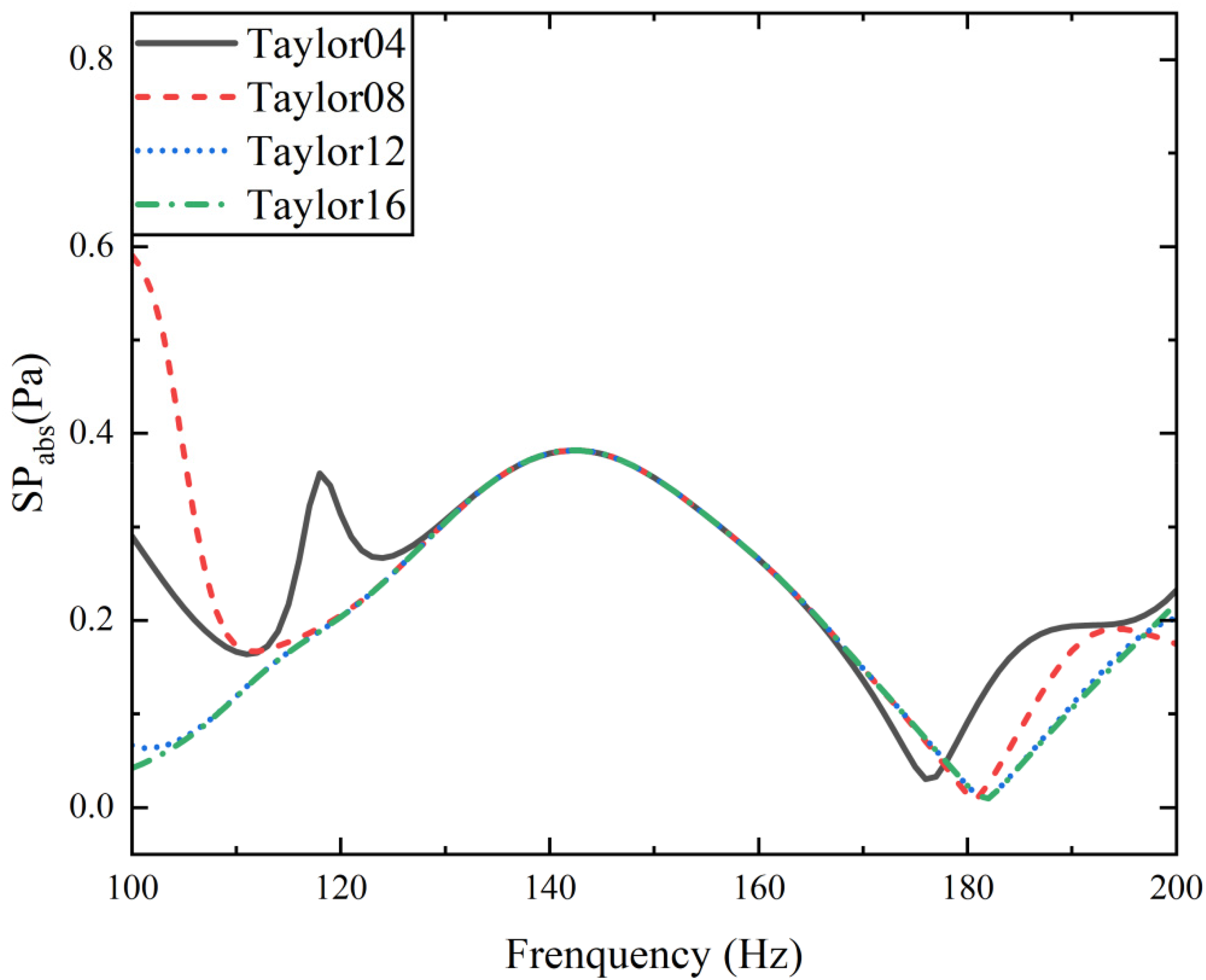
The sound pressure at calculation point (12 m, 2 m) using IGABEM with Taylor expansion in the [100, 200] Hz range.

From the simulation results, it can be seen that the calculation results converge with the increase in the number of Taylor expansion terms. Since the fixed expansion point of a given frequency interval is located at the midpoint of the interval, there are significant differences in the sound pressure values obtained from different Taylor expansion terms at both ends of the interval, while better consistency is observed in the center of the interval. In order to solve this problem, the frequency range is subdivided into two sub-intervals from the mid-frequency expansion point. The simulation calculation results of [100, 150] Hz are shown in Figure 8.

Figure 8.

The sound pressure at calculation point (12 m, 2 m) using IGABEM with Taylor expansion in the 100–150 Hz range.

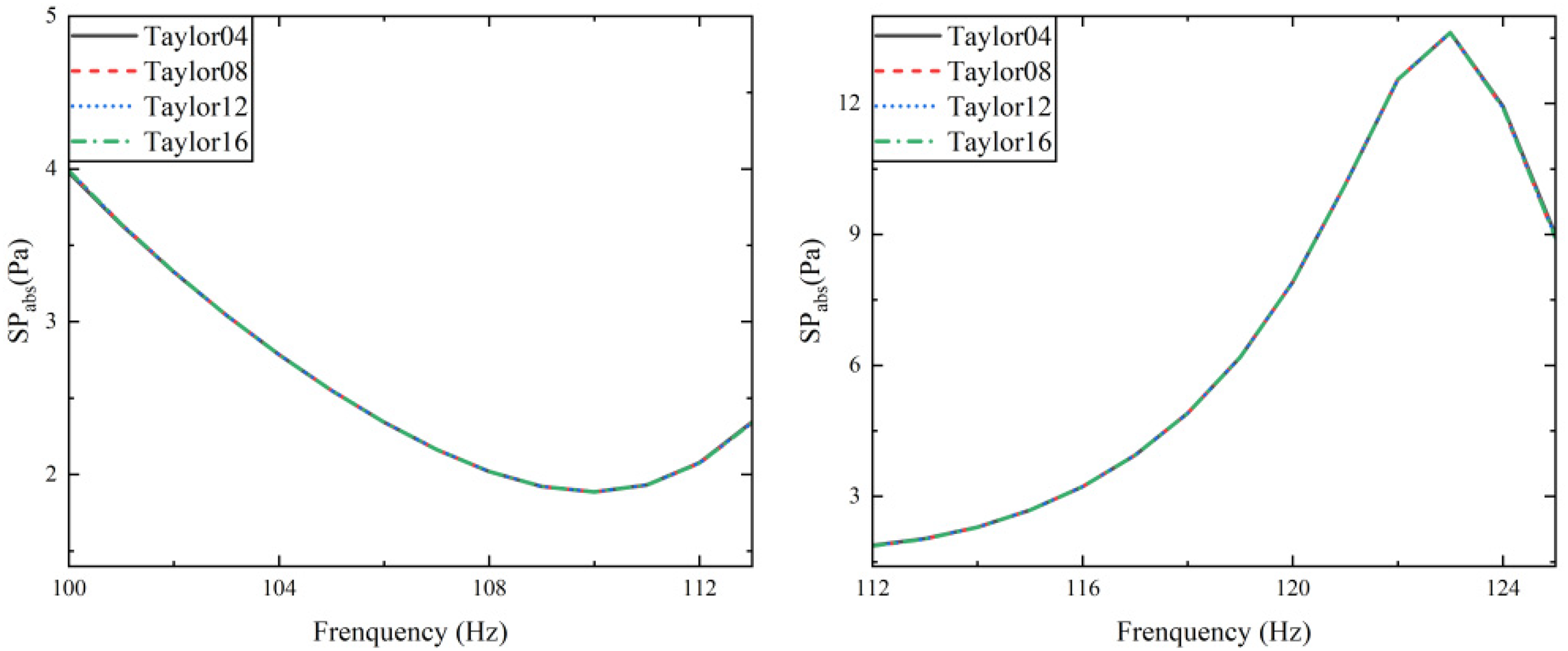
We can see that in the frequency range of [100, 150] Hz, except that the result of the Taylor expansion term number of 4 is different from the other terms, the other three curves converge to almost the same one, that is, the sound pressure calculated by Taylor expansion terms of 8, 12, and 16 is almost the same. Specifically, when the number of terms in the Taylor series expansion is greater than or equal to 8, the calculation results are more accurate. This is because when the Taylor expansion is 4 terms, the calculation error is large. Therefore, to ensure the accuracy of the calculation results, we use a Taylor expansion term of no less than 8 when comparing the simulation calculation results. Since the overall sound pressure value of the simulation results is small, a small difference will cause a large error. To make the results more accurate, we continue to subdivide the frequency. In the 25 Hz frequency range, the simulation results are as follows:

Figures 7, 8, and 9 show that as the frequency interval is subdivided, the results gradually converge, and the sound pressure value becomes more accurate, proving the effectiveness of the interval subdivision. In this model, when the frequency segment is divided into [100, 125] Hz and [125, 150] Hz, the convergence rules of the two subset curves are basically the same. Therefore, for this model, the calculation result is more accurate when the frequency segment is 25 Hz.

Figure 9.

The sound pressure at calculation point (12 m, 2 m) using IGABEM with Taylor expansion in two different frequency subintervals for top curved sound barrier.

Deep neural network prediction

After determining the appropriate expansion range of the Taylor series (not less than 8) and the fixed point expansion frequency range (within 25 Hz), we use a Taylor expansion term of 10 and a range of 25 Hz to calculate the sound pressure value of the model at the inspection point (12 m, 2 m), which can ensure the accuracy of the calculation. In order to obtain sufficient data for the neural network training set, we calculate data within multiple 25 Hz continuous frequency segments, such as calculating 12 frequency bands of 25 Hz from [100, 400] Hz, and input the calculation results into the built deep neural network for training. The frequency step size of 5 HZ is used to obtain the training set to reduce the calculation time. Since the data errors at both ends of the frequency band are large when the Taylor series is expanded, we average the data results at the connection of the frequency points. In the fitting process of the left and right frequency bands, the data points are closer to the true values. Figure 10 shows the calculation results of each frequency in the [100, 400] Hz frequency band.

Figure 10.

The sound pressure calculated every 25 Hz frequency band in the range of [100, 400] Hz with a step size of 4.

Then, the above calculation results are input into the DNN model for training. When using neural networks, it should be noted that the training process is inherently random, which may cause the generated mapping function and subsequent calculation output to vary. If a poorly trained mapping function leads to large errors, multiple training iterations should be performed to evaluate the stability of the model. If some training results have too many errors, it is recommended to refine the training dataset and retrain the DNN model to enhance its generalization ability and prediction accuracy. After the neural network training data is completed, we can predict the sound pressure value of any frequency point within [100, 400] Hz. The evaluation indicators of the neural network prediction results are calculated as follows:

In Table 2, it can be seen that the MSE, MAE, and SMAPE evaluation indicators are all small, and R² is close to 1, indicating that the DNN prediction model is better. Comparing the Taylor expansion with the neural network calculation results, the resulting curve is shown in Figure 11.

Figure 11.

Comparison of results calculated by DNN and Taylor series expansion for model of top curved sound barrier.

Table 2.

Evaluation index calculation results for model of top curved sound barrier.

MSE	MAE	SMAPE	R 2
0.0000361	0.00452	3.46%	0.996405

As can be seen from Figure 11, the difference between the result value calculated by the neural network and the Taylor calculation is small. When we train a suitable neural network model, its calculation time is only 3.16752 s, which greatly speeds up the calculation.

Sound scattering of cylindrical sound barriers

Studies have shown that when sound-absorbing or flexible sound barriers are used, cylindrical noise reduction effects are stronger. This section analyzes the scattering of sound waves by cylindrical sound barriers under ground reflection conditions. As shown in Figure 12, the model is constructed using an isogeometric model, defined by 12 control points and discretized into 859 constant boundary elements, with a top circle radius of 0.8 m. The observation point is positioned at (12 m, 2 m), while the remaining numerical simulation parameters are identical to those in Table 1.

Figure 12.

Cylindrical sound barrier constructed using IGABEM under plane wave excitation.

After constructing the sound barrier model, we performed Taylor series expansion on IGABEM. When calculating the model, the Taylor series with 4, 8, 12, and 16 items were used for expansion. Through the frequency division calculation results, we finally determined that the frequency was in the range of [100, 125] Hz, and the calculation results were relatively accurate. The convergence rules of the two sub-intervals of [100, 125] Hz and [125, 150] Hz were also consistent. Therefore, in our subsequent calculations, the frequency segment was selected within the range of 25 Hz for calculation, and the simulation calculation results are shown in Figure 13.

Figure 13.

The sound pressure at calculation point (12 m, 2 m) using IGABEM with Taylor expansion in two different frequency subintervals for cylindrical sound barrier.

As can be seen from Figure 13, the four curves show a high degree of consistency, indicating that no matter how many expansion terms are used, the change in the sound pressure value is minimal. It is worth noting that the fixed frequency expansion point in each frequency sub-interval is located at the midpoint of the corresponding sub-interval. Then, we use a frequency point with a step size of 5 Hz and a Taylor expansion term of 10 for calculation. The calculation results are used as a training set and input into the DNN model for training. After the training is completed, we can use the model to obtain the predicted sound pressure value with a frequency interval of 1 Hz, the evaluation indicators of the neural network prediction results are calculated in Table 3, which shows that combining the boundary element method with the deep neural network method can significantly improve the calculation efficiency and accuracy:

Table 3.

Evaluation index calculation results for model of cylindrical sound barrier.

MSE	MAE	SMAPE	R 2
0.0027	0.0402	8.58%	0.989322

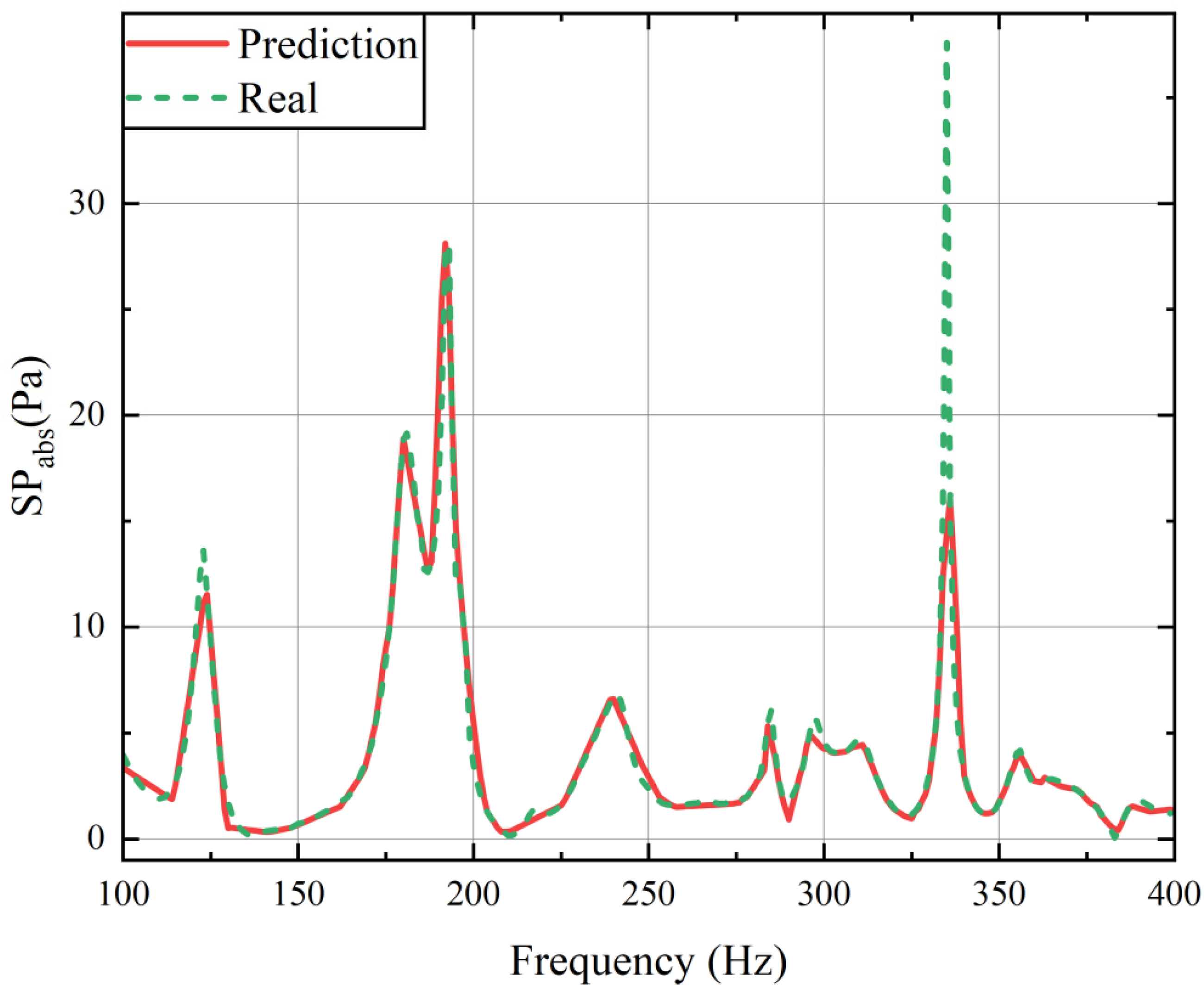
Compare the predicted sound pressure value with the simulated sound pressure value with a frequency of 1 Hz for verification. The comparison result is shown in Figure 14.

Figure 14.

Comparison of results calculated by DNN and Taylor series expansion for model of cylindrical sound barrier.

The sound pressure changes in a complex manner within a wide frequency range, and the data predicted by the neural network can fit the trend of sound pressure changes well. It is further speculated that for sound barriers with complex shapes, the effect of neural network prediction is relatively weak due to the complexity of the actual sound pressure conditions.

Sound scattering of trapezoidal sound barriers

The trapezoidal arc top shape has been put into use on some highway sections because of its good noise reduction performance, environmental coordination, beautiful appearance, and easy manufacturing, installation, and maintenance. As shown in Figure 15, we use the isogeometric model to simplify the trapezoidal sound barrier model, which is discretized into 1289 constant boundary elements, with the observation point located at (12 m, 2 m).

Figure 15.

Trapezoidal sound barrier constructed using IGABEM under plane wave excitation.

As in the calculation steps of sections “Sound scattering of top curved sound barrier” and “Sound scattering of cylindrical sound barriers,” we continuously subdivide the frequency, and the final frequency range is within 13 Hz. The curve of the model's sound pressure calculation result converges well. The [100, 113] Hz frequency range and [112, 125] Hz frequency range are simulated, respectively. From the results, it can be seen that the simulation results of the two sub-frequency ranges divided by 13 Hz as the fixed expansion point have highly converged. The simulation curves of the two sub-frequencies are shown in Figure 16.

Figure 16.

The sound pressure at calculation point (12 m, 2 m) using IGABEM with Taylor expansion in two different frequency subintervals for trapezoidal sound barrier.

Considering that the model has high accuracy in the 13 Hz frequency range but a small calculation range, we calculated the simulation results of [100, 400] Hz in the 13 Hz frequency band with a 4 Hz step size and 10 Taylor expansion frequency points. For the sound pressure values that are repeatedly calculated at both ends of the frequency band, we used the averaging method to fit the two calculation results, which not only provides more training data for DNN but also effectively reduces the impact of the errors at both ends of the frequency band. When the calculation range is [100, 400] Hz and the step length is 1 Hz, the prediction results of the neural network and the results calculated by Taylor expansion are shown in Table 4.

Table 4.

Evaluation index calculation results for model of trapezoidal sound barrier.

MSE	MAE	SMAPE	R 2
2.348071906	0.402252501	11.4%	0.89758763

Since the model is relatively complex, when the sound pressure is incident on the sound barrier, the sound pressure value changes more complexly, and false eigenfrequency points are difficult to avoid. Therefore, the problem of extreme values appears in the calculation process. Therefore, when using evaluation indicators, some indicators are easily affected by extreme values, resulting in poor results. This is the disadvantage of these evaluation indicators. For example, MSE will be affected by outliers and grow exponentially with the increase of errors. Below, we compare the predicted value of the neural network with the calculation result of the Taylor expansion to further illustrate this problem. The comparison results are shown in Figure 17.

Figure 17.

Comparison of results calculated by DNN and Taylor series expansion for model of trapezoidal sound barrier.

From Figure 17, we can see the irregularity of the sound pressure variation in the frequency range of [100,400] Hz, and extreme values appear at some special frequency points. When dealing with such extreme value problems, the neural network will use a smoother curve for fitting, and the numerical results are more in line with engineering reality.

Conclusion

In the computation of two-dimensional acoustic models, an excessive number of discretized elements, an overly large Taylor series expansion order, or an extended frequency range can significantly increase computational cost and processing time. In response to these challenges, this study proposes an accelerated isogeometric boundary element method based on Taylor series expansion, integrated with deep neural networks for efficient acoustic field calculations. Validation through acoustic scattering cases involving sound barriers with different topological structures demonstrates that increasing the number of Taylor expansion terms and refining the frequency intervals enhance the accuracy and convergence of the results. Additionally, the DNN model facilitates rapid prediction of sound pressure values at any frequency point within a given range, significantly reducing computational time and cost compared to traditional BEM approaches, thereby improving computational efficiency. Moreover, the proposed method offers the following key advantages, which are also reflected in the application process:

When the Taylor series is expanded, the error of the numbers at both ends of the frequency segment is large due to the expansion at the middle point of the frequency; when the neural network is input for training, the neural network lacks training data for the numbers at both ends of the data, so the error of the numbers at both ends of the data is further increased. We merge multiple frequency segments and make a preliminary fit of the numbers at both ends of the data, so the data accuracy is further improved.

The more complex the model is, the more complex the actual sound pressure changes. The appearance of extreme values leads to less ideal evaluation index values. The application of neural networks smoothes the extreme values, and the final effect is more in line with the sound pressure changes in actual engineering.

The proposed method provides an effective solution for acoustic analysis involving complex geometric structures, and can be extended to three-dimensional problems in future research.