Calculation of interphase elastic properties of esterified cellulose nanocrystal/epoxy bio-nanocomposites using analytical and finite element methods

Abstract

In this study, analytical models and numerical finite element analysis (FEA) were used to accurately determine the interphase properties and elastic modulus of both untreated and esterified cellulose nanocrystals (CNC)/epoxy bio-nanocomposites. This was achieved by incorporating an interphase region around the CNC particles, with properties that vary between those of the nanofiller and the matrix. Experimental techniques for measuring interphase properties, such as atomic force microscopy and nanoindentation, are useful but sensitive to sample preparation and limited to certain materials, which makes modelling a valuable alternative. Random 2D and 3D representative volume elements (RVEs) were generated using Digimat-FE and imported into ANSYS to determine the behaviour of nanocomposite under load. The elastic moduli values from analytical and FEA models, which included the interphase region, fell within the range of experimental variation. The results showed that the modulus increased with CNC loading from 2.5 wt% to 5 wt% and that nanofiller treatment enhanced the modulus and increased the interphase thickness. For excessive esterification, there was a weakening effect on the composite that the analytical models failed to accurately predict. ANSYS response surface optimization was used to determine the optimal geometries and material properties for the FEA model, leading to accurate behaviour. Latin hypercube sampling (LHS) was used to explore the design space, and the optimal geometry was identified with a 6 nm interphase thickness, an aspect ratio of 10, a CNC modulus of 0.66 MPa, and an interphase modulus of 1.28 GPa. The 2D FEA RVE models struck a balance between accuracy and computational costs for treated nanoparticles.

Graphical abstract

This is a visual representation of the abstract.

Introduction

Recent advancements in biomaterials research have highlighted the potential of nanocellulose (NC), a material with impressive properties such as biodegradability, biocompatibility, optical performance, strength, and surface chemistry, as an ideal candidate for reinforcing polymer composites. ¹ Using NC as reinforcement fillers in polymer matrices, instead of synthetic fillers, can contribute to the UN's Sustainable Development Goal (SDG) 12. SDG 12 aims for sustainable consumption and production patterns, promoting resource efficiency, waste reduction, and sustainable practices. ² The use of NC aligns with these goals by promoting sustainability and reducing reliance on synthetic fillers. Various forms of NC, including cellulose nanofibers (CNF), cellulose nanocrystals (CNC), nano-fibrillated cellulose (NFC), and bacterial cellulose, can be derived from a range of sources like plants, microorganisms, and cellulose-rich aquatic animals.^1,3 Extraction techniques, which include the use of homogenizers, microfluidizers, or grinders, influence the unique properties of NC. These methods produce CNF by disintegrating cellulose fibres while maintaining their length and crystalline structure. Acid hydrolysis is used to produce CNC by removing the amorphous regions through acid/alkali hydrolysis, resulting in rod-like CNCs with lengths typically ranging from 200 nm to 800 nm and diameters around 10 nm to 50 nm.^4,5 Enzymatic treatment with enzymes like cellulase offers an alternative method for obtaining CNCs. ⁶

Despite the favourable characteristics of NC, there are certain limitations when using it as a nanofiller modifier for polymers. The surface chemistry of NC includes free hydroxyl groups that attract water, leading to less favourable properties of polymer/NC composites. Additionally, most polymer matrices exhibit hydrophobic behaviour, which hampers the dispersion and bonding of hydrophilic NC. Furthermore, due to the substantial aspect ratio of NC, the high surface energy results in attractive forces between adjacent NC particles, leading to agglomeration. ⁷ To mitigate these limitations, chemical treatments like esterification, ⁸ and silanisation ⁹ can be employed. These treatments derivatise the hydroxyl groups on NC, making the NC more hydrophobic.

When incorporating nanofillers into a polymer matrix, the resulting composite's properties depend on the effectiveness of load transfer at the fibre/polymer interface. This interaction is influenced by the relative size of the polymer chain, represented by the ratio 2Rg/D. Here, Rg represents the radius of gyration, while D is the diameter of the cylindrical nanofillers. The radius of gyration, Rg, is defined as the square root of the average squared distance of any point in the polymer chain from its centre of mass. ¹⁰ If 2Rg/D < 1, the polymer chains fail to fully envelop the nanofiller, resulting in poor load transfer efficiency at the interface. Conversely, when the nanofillers’ diameter (D) is smaller than twice the radius of the gyration of the polymer chain (2Rg/D > 1), load transfer improves as the polymer chains can effectively surround the nanofillers. Therefore, smaller particles lead to enhanced mechanical properties. ¹¹

In the proximity of the nanofillers, the polymer chains experience perturbations due to network-like structures formed around the nanofillers. These structures arise when polymer chains adsorbed on the nanofillers’ surface create loop formations. These loops facilitate chain entanglement with neighbouring polymer chains, restricting the mobility of the polymer chains. As a result, the packing density increases, and the free volume between polymer chains decreases. ¹² This phenomenon forms a region called an interphase, extending only a few nanometres from the nanofillers' surface. Beyond this region, the properties resemble those of the bulk polymer.^13–15 When nanofillers are surface functionalised, there are more adsorption points between the polymer chains and nanofillers which results in a thicker interphase. The formation of the loop structures, the subsequent entanglement, and the increase in the thickness of interphase due to surface functionalisation are shown in Figure 1.

Figure 1.

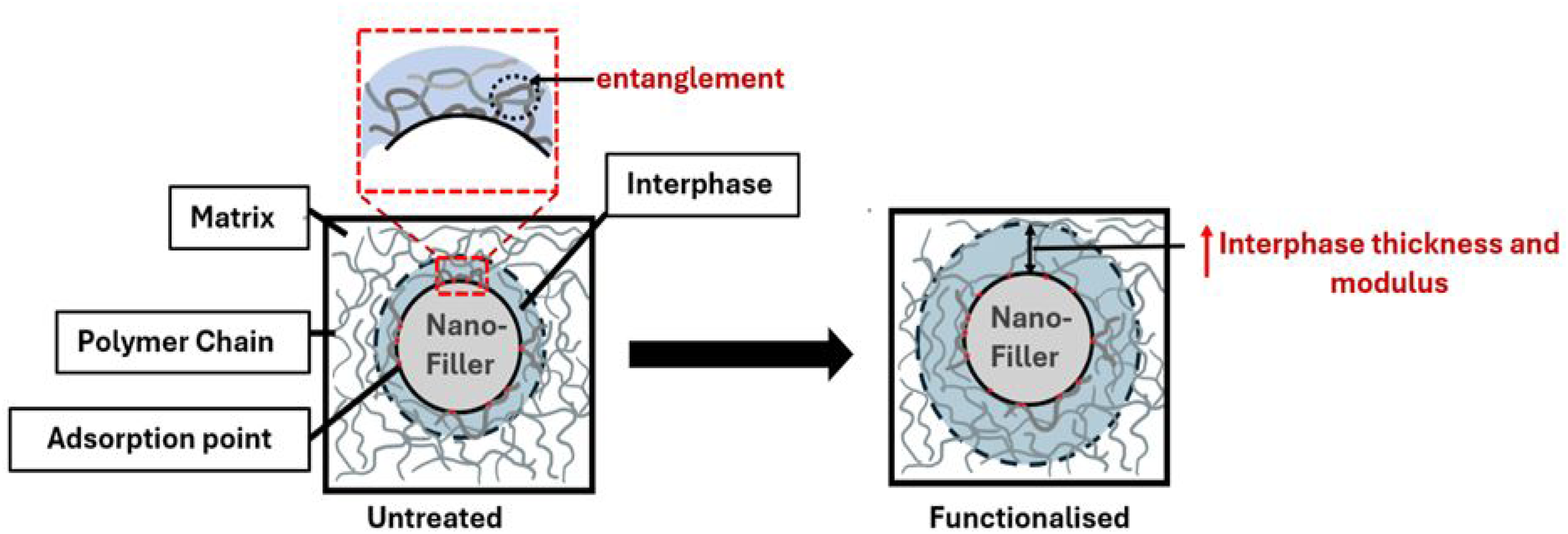
Formation of the interphase region when nanofillers are added to polymer matrices, showing the loop structures that cause entanglement and the increase in interphase thickness when the nanofillers are surface-functionalized.

Experimental measurement of interphase properties presents challenges, particularly in cases involving matrix-induced phenomena. Researchers have employed techniques such as atomic force microscopy and nanoindentation to explore this region and correlate load–displacement curves with the matrix, nanofillers, and interphase regions. In a study by Kim et al., ¹⁶ three interphase characterization methods—nanoindentation, nanoscratch, and thermal capacity jump measurements—were explored. The nanoindentation tests exhibited significant specimen-to-specimen variations and lacked sensitivity in distinguishing the effects of different silane coupling agents in glass fibre/polymer resin composites. On the other hand, thermal capacity jump and nanoscratch measurements showed consistent trends, the former tended to predict larger interphase thickness values. These experimental techniques, while insightful, are potentially affected by sample preparation and are applicable only to specific material classes and properties.

Various methods to determine the interphase properties of nanocomposites have been attempted in the past. Molecular dynamics (MD) has been successfully used to infer the properties of the interphase region in nanoparticles. Taheri et al. ¹⁷ determined the properties of the interphase region in carbon nanocones/polyethylene (PE) composites using molecular dynamics simulations. They then integrated these properties into a finite element model, which yielded accurate results. Their study highlighted the significant impact of the geometrical parameters of carbon nanocones on the interphase properties and the overall mechanical strength of the nanocomposites. Talebi et al. ¹⁸ developed a computational library that incorporated various libraries from molecular dynamics and finite element methods to predict the fracture and mechanical properties of multiscale composites.

Given that MD models are time-consuming to run, researchers have been exploring faster methods, such as closed-form analytical models or numerical finite element models, to efficiently study and predict the behaviour of nanocomposites. Various analytical models, including Halpin-Tsai ¹⁹ and Takayanagi, ²⁰ have been used to calculate the modulus of reinforced polymer composites. However, these models overlook the interphase region present in polymer nanocomposites (PNCs), leading to inaccurate modulus predictions. Ghasemi et al. ²¹ incorporated the interphase region into the Takayanagi model, resulting in more accurate modulus predictions for nanocomposites. Furthermore, Ji et al. ²² considered both agglomeration and the interphase region in their modified Takayanagi model, achieving improved accuracy in their results. While these models offer fast solutions, they have limitations when dealing with intricate composites, particularly in simulating the complex geometries of nanoparticles. In addition, their simplicity can sometimes lead to calculations that violate established principles of material symmetry in stiffness and compliance tensors. ²³

Finite element analysis (FEA) provides a numerical approach to address these shortcomings by discretizing the problem domain into small elements and solving the governing equations. FEA enables the inclusion of interphase regions and the examination of stress and strain fields and their distributions, along with the exploration of the mechanical characteristics of the nanocomposites. FEA models are generally faster than MD models due to the different scales and types of problems they address. FEA focuses on macroscopic properties, using approximations to speed up computations and improve efficiency, making it highly scalable for large systems. In contrast, MD models atomic-level interactions in detail, requiring significantly more computational power and slowing down as the number of atoms increases. Narita et al. ²⁴ used representative volume elements (RVEs) to study the mechanical behaviour of CNF/Epoxy composites without considering an interphase between the CNF and the matrix. They found that the Young's modulus obtained from the RVE tends to be higher than the experimental results. Xie et al. ²⁵ determined the flexural properties of CNF/Epoxy composites using FEA without considering the interphase region and found that the experimental values for flexural modulus were higher than the ones obtained from the FE analysis. They concluded that existing analytical models for short-fibre-reinforced composites were not sufficiently accurate. Vattathurvalappil et al. ²⁶ used an RVE that considered the interphase around spherical nano iron oxide. They found that the results from FEA models with interphase region included agreed well with the experimental results while those without interphase did not.

Due to the computational cost associated with simulating an entire PNC microstructure, RVE homogenisation techniques are commonly used to model PNCs. These RVEs have the capability for studying a material's macroscopic behaviour at its microstructure level. Through the analysis of an RVE that is statistically representative of the entire material, effective properties such as modulus, conductivity, or strength can be extracted for application at macro scales. To the author's best knowledge, studies that validate finite element analysis results using interphase properties derived from closed-form analytical solutions, supported by experimental data from nanocomposite tests, were either lacking or non-existent in the literature. Additionally, research on the effects of esterification treatment on the interphase and nanocomposite properties of nanocellulose was also scarce. Therefore, this study aimed to investigate the impact of the interphase region on the accuracy of two-dimensional (2D) and three-dimensional (3D) FEA RVE models of CNC/Epoxy. It also explored how esterification treatment influences interphase properties and the relative modulus of the nanocomposite while addressing the limitations of analytical models and how FEA can overcome these challenges. The results showed that both analytical and finite element analysis (FEA) models, which included the interphase region, provided more accurate results in comparison with the experimental data. However, for high degrees of esterification, the analytical models failed to accurately predict the modulus of the nanocomposite, whereas the FEA RVE models provided accurate predictions. It was shown that the 2D FEA models provided a balance between accuracy and computational costs for PNCs modified with treated particles.

Methods for calculating the elastic modulus of nanocomposites

Analytical methods

Modified Takayanagi model

The elastic modulus of polymer nanocomposites depends on various factors associated with both the polymer and reinforcements. These factors include nanofiller loading, nanofiller aspect ratio, particle alignment, and the interphase region. Several models have been proposed to effectively predict the elastic properties of PNCs. One of these models is the Takayanagi model, ²⁰ which expresses the Young's modulus of composite as follows:

$$E=E_{\mathrm{m}}{\left[(1-A)+{\displaystyle \frac{B}{(1-A)+B{\displaystyle \frac{E_{\mathrm{f}}}{E_{\mathrm{m}}}}}}\right]}^{-1}$$

(1)

where $E_{\mathrm{f}}$ and $E_{\mathrm{m}}$ are the tensile modulus of the filler and matrix, respectively, and $A=B=\sqrt{{\varphi }_{\mathrm{f}}}$ where ${\varphi }_{\mathrm{f}}$ represents the nanofillers volume fraction. In this model it was assumed the nanofillers and matrix are perfectly bonded and when the composite is subjected to tension, some of the lines of force within the sample pass exclusively through the matrix, while others traverse both the matrix and the nanofillers in series. ²²

Considering the interphase region and the aspect ratio of the particle, Ghasemi et al. ²¹ developed the following relationship for Young's modulus using the rule of mixtures:

$$E=E_{\mathrm{m}}{\left[(1-\alpha )+{\displaystyle \frac{\beta }{H}+{\displaystyle \frac{\alpha }{a}+{\displaystyle \frac{\beta }{(1-\alpha )+\beta {\displaystyle \frac{E_{\mathrm{f}}}{E_{\mathrm{m}}}}}}}}\right]}^{-1}$$

(2)

where: $\alpha =\sqrt{{\varphi }_{\mathrm{eff}}}$ , $\beta =\sqrt{{\varphi }_{\mathrm{f}}}$ , $H=\frac{E_{\mathrm{i}}}{E_{\mathrm{m}}}$

In equation (2), $a=l/d$ represents the aspect ratio of the particle where l is the length and d is the particle diameter, ${\varphi }_{\mathrm{f}}$ is the nanofillers loading (wt%), and $E_{\mathrm{i}}$ represents the interphase modulus. The interphase volume fraction can be obtained from the following function ²¹ :

$${\varphi }_{\mathrm{i}}={\varphi }_{\mathrm{f}}\left[{\left(1+2{\displaystyle \frac{t}{d}}\right)}^2-1\right]$$

(3)

where t is the interphase thickness.

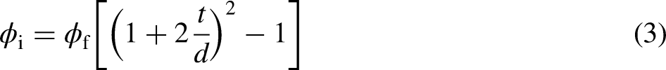
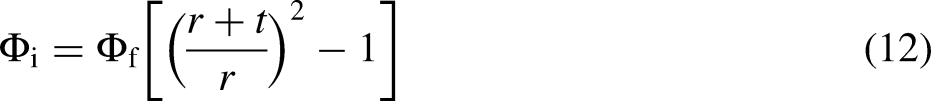
When calculating the effective loading of cellulose nanocrystals (CNCs), it is crucial to account for both the volume fractions of CNCs and the interphase. These factors significantly influence the reinforcement of nanocomposites. ${\varphi }_{\mathrm{eff}}$ is effective loading and can be determined using the following expression:

$${\varphi }_{\mathrm{eff}}={\varphi }_{\mathrm{f}}+{\varphi }_{\mathrm{i}}={\varphi }_{\mathrm{f}}{\left(1+2{\displaystyle \frac{t}{d}}\right)}^2$$

(4)

by substituting equations (3) and (4) into equation (2), the relative modulus $E_{\mathrm{r}}=\frac{E}{E_{\mathrm{m}}}$ can be expressed as ²¹ :

$$\begin{array}{rl}& E_{\mathrm{r}}=[\left(1-\sqrt{{\varphi }_{\mathrm{f}}{\left(1+2{\displaystyle \frac{t}{d}}\right)}^2}\right)+{\displaystyle \frac{E_{\mathrm{m}}\sqrt{{\varphi }_{\mathrm{f}}}}{E_{\mathrm{i}}}+{\displaystyle \frac{\sqrt{{\varphi }_{\mathrm{f}}{\left(1+2{\displaystyle \frac{t}{d}}\right)}^2}}{a}}}\\ & {+{\displaystyle \frac{\sqrt{{\varphi }_{\mathrm{f}}}}{\left(1-\sqrt{{\varphi }_{\mathrm{f}}{\left(1+2{\displaystyle \frac{t}{d}}\right)}^2}\right)+{\displaystyle \frac{\sqrt{{\varphi }_{\mathrm{f}}}{E}_{\mathrm{f}}}{E_{\mathrm{m}}}}}}]}^{-1}\end{array}$$

( 5)

Ji model

Another model derived from the Takayanagi model is the Ji model ²² presented in equation (6).

$$E_{\mathrm{r}}={\left[(1-{\alpha }_{\mathrm{i}})+{\displaystyle \frac{{\alpha }_{\mathrm{i}}-\beta }{(1-{\alpha }_{\mathrm{i}})+{\displaystyle \frac{{\alpha }_{\mathrm{i}}(H-1)}{\ln (H)}}}+{\displaystyle \frac{\beta }{(1-{\alpha }_{\mathrm{i}})+{\displaystyle \frac{({\alpha }_{\mathrm{i}}-\beta )(H+1)}{2}+\beta {\displaystyle \frac{E_{\mathrm{p}}}{E_{\mathrm{m}}}}}}}}\right]}^{-1}$$

(6)

${\alpha }_{\mathrm{i}}$ depends on the shape of the particles. ${\alpha }_1$ , ${\alpha }_2$ , and ${\alpha }_3$ are for nanofillers with spherical ( $i=1$ ), platelet ( $i=2$ ), and cylindrical $(i=3$ ) shapes and they are defined by:

$${\alpha }_1=\sqrt{{\left({\displaystyle \frac{t}{r}+1}\right)}^3}{\mathrm{\Phi }}_{\mathrm{f}}$$

(7)

$${\alpha }_2=\sqrt{\left({\displaystyle \frac{2t}{d}+1}\right)}{\mathrm{\Phi }}_{\mathrm{f}}$$

(8)

$${\alpha }_3=\sqrt{{\left({\displaystyle \frac{t}{r}+1}\right)}^2}{\mathrm{\Phi }}_{\mathrm{f}}$$

(9)

The volume fractions of the interphase region for a sphere, platelet, and cylinder were given by Yanovshy et al. ²⁷ in equation (10) to (12), respectively.

$${\mathrm{\Phi }}_{\mathrm{i}}={\mathrm{\Phi }}_{\mathrm{f}}\left[{\left({\displaystyle \frac{r+t}{r}}\right)}^3-1\right]$$

(10)

$${\mathrm{\Phi }}_{\mathrm{i}}={\mathrm{\Phi }}_{\mathrm{f}}\left({\displaystyle \frac{2t}{d}}\right)$$

(11)

$${\mathrm{\Phi }}_{\mathrm{i}}={\mathrm{\Phi }}_{\mathrm{f}}\left[{\left({\displaystyle \frac{r+t}{r}}\right)}^2-1\right]$$

(12)

The relationship between Young's modulus of PNCs and the volume fractions of the interphase proposed by Yanovshy et al. ²⁷ assumed that the interphase region surrounded the outer surface of the nanofiller. They also proposed an equation for the relationship between the relative Young's modulus of PNCs and the volume fraction of the interphase and nanofillers which considers the nonlinearities due to agglomeration.

$$E_{\mathrm{r}}=1+11({\varphi }_{\mathrm{f}}+{\varphi }_{\mathrm{i}}{)}^{1.7}$$

(13)

By substituting equation (10) to (12) into equation (7) to (9), $\alpha$ for all nanofillers shapes can be represented as:

$$\alpha =\sqrt{{\varphi }_{\mathrm{eff}}}=\sqrt{{\varphi }_{\mathrm{f}}+{\varphi }_{\mathrm{i}}}$$

(14)

Rearranging equation (13) and substituting into equation (14) gives:

$$\alpha ={\left({\displaystyle \frac{E_{\mathrm{r}}-1}{11}}\right)}^{0.294}$$

(15)

where $E_{\mathrm{r}}$ is the experimental relative Young's modulus.

The interphase layer between the polymer matrix and nanoparticles can be segmented into $\mathrm{n}$ layers. Within these layers, the mechanical properties gradually transition from the nanoparticle properties to the polymer matrix properties. Assuming a constant thickness for all interphase layers, the thickness of the kth layer is given by:

$$t_k={\displaystyle \frac{t}{n}}$$

(16)

X is defined as the distance from the nanoparticle surface (x = 0) to the polymer matrix (x = t). The distance x for the central point of the k-th layer to the nanoparticle surface can be expressed as:

$$x_k={\displaystyle \frac{t_k(k-1)}{2}}$$

(17)

Zare et al. ²⁸ assumed that Young's modulus of the interphase is varying according to a power function Y represented as:

$$E_k=E_{\mathrm{f}}-(E_{\mathrm{f}}-E_{\mathrm{m}}){\left({\displaystyle \frac{x_k}{t}}\right)}^Y$$

(18)

The parameter Y depends on various characteristics of the interphase between polymer and nanofillers. A higher value of Y indicates a thicker interphase between the polymer and nanofillers, resulting from more adsorption points between the polymer chains and nanofillers. Additionally, a higher value signifies stronger interphase interaction and more robust interphase regions. Conversely, when Y equals 0, it implies that there are no interphase regions present between the particles and the matrix and $E_{\mathrm{i}}$  =  $E_{\mathrm{m}}$ .

By assuming that $E_{\mathrm{i}}$ varies linearly between the nanofiller and matrix, the average value of $E_{\mathrm{i}}$ can be found by substituting $x_k=\frac{t}{2}$ into equation (18) to give the following expression:

$$E_{\mathrm{i}}=E_{\mathrm{f}}-(E_{\mathrm{f}}-E_{\mathrm{m}}){0.5}^Y$$

(19)

Therefore, the ratio of interphase module to matrix modulus, $H=\frac{E_{\mathrm{i}}}{E_{\mathrm{m}}},$ can be expressed by:

$$H={\displaystyle \frac{[E_{\mathrm{f}}-(E_{\mathrm{f}}-E_{\mathrm{m}}){0.5}^Y]}{E_{\mathrm{m}}}}$$

(20)

By substituting equations (15) and (20) into equation (6), the final equation for the relative Young's modulus for the Ji model is obtained as shown in equation (21).

$$\begin{array}{rl}& E_{\mathrm{r}}=[\left(1-{\left({\displaystyle \frac{E_{\mathrm{r}}-1}{11}}\right)}^{0.294}\right)+{\displaystyle \frac{{\left({\displaystyle \frac{E_{\mathrm{r}}-1}{11}}\right)}^{0.294}-\sqrt{{\varphi }_{\mathrm{f}}}}{\left(1-{\left({\displaystyle \frac{E_{\mathrm{r}}-1}{11}}\right)}^{0.294}\right)+{\displaystyle \frac{{\left({\displaystyle \frac{E_{\mathrm{r}}-1}{11}}\right)}^{0.294}\left({\displaystyle \frac{[E_{\mathrm{f}}-(E_{\mathrm{f}}-E_{\mathrm{m}}){0.5}^Y]}{E_{\mathrm{m}}}-1}\right)}{\ln \left({\displaystyle \frac{(E_{\mathrm{f}}-(E_{\mathrm{f}}-E_{\mathrm{m}}){0.5}^Y)}{E_{\mathrm{m}}}}\right)}}}}\\ & {+{\displaystyle \frac{\sqrt{{\varphi }_{\mathrm{f}}}}{\left(1-{\left({\displaystyle \frac{E_{\mathrm{r}}-1}{11}}\right)}^{0.294}\right)+{\displaystyle \frac{\left({\left({\displaystyle \frac{E_{\mathrm{r}}-1}{11}}\right)}^{0.294}-\sqrt{{\varphi }_{\mathrm{f}}}\right)\left({\displaystyle \frac{[E_{\mathrm{f}}-(E_{\mathrm{f}}-E_{\mathrm{m}}){0.5}^Y]}{E_{\mathrm{m}}}+1}\right)}{2}+\sqrt{{\varphi }_{\mathrm{f}}}{\displaystyle \frac{E_{\mathrm{f}}}{E_{\mathrm{m}}}}}}}]}^{-1}\end{array}$$

( 21)

Numerical method

Homogenisation process

Homogenisation theory relies on the assumption that continuum mechanics theory provides an appropriate framework for describing the overall mechanical behaviour of a heterogeneous medium. Although the medium is microscopically heterogeneous, its heterogeneities are much smaller than a relevant macroscopic characteristic length. From a macroscopic perspective, these heterogeneities are indistinguishable, leading to the medium exhibiting macroscopically homogeneous behaviour. As a result, it is reasonable to assume periodicity in this context. ²⁹ For an equilibrium problem involving complex heterogeneities, the media is redefined as a boundary value problem using Representative volume elements (RVEs) involving stress and strain tensor fields. Subsequently, this redefined behaviour is transferred back to the macroscopic scale, where it is treated as an equivalent homogeneous medium shown in Figure 2. The RVE can be defined as a small volume within the macroscopic body. However, it must still be large enough to account for microstructural features. ³⁰

Figure 2.

Homogenisation process showing applied boundary condition to the heterogenous medium to obtain the homogeneous medium.

Size of RVE

While the size of the RVEs is inconsequential for a homogeneous material, it becomes crucial for heterogeneous materials. The primary premise of the homogenisation theory using RVEs is the statistical homogeneity of the medium. Statistical homogeneity implies that the characteristics of the microstructure remain consistent throughout the material at the macroscale. When particles are dispersed randomly within a medium, the medium can be considered homogeneous. The implication of this random distribution is that the macroscale attributes of a material, which has a statistically uniform microstructure, are assumed to be unaffected by the specific location at the macroscale where the material's properties are examined. ³¹ The appropriate size of an RVE depends significantly on material characteristics, including the number of phases and their spatial distribution. The chosen RVE must strike a balance: it should include enough heterogeneities to be statistically representative, yet remain small enough to function as a volume element of continuum mechanics. ³⁰

Equivalent constitutive relation

To characterise a macroscopically uniform medium, macro-stress and macro-strain are calculated by averaging the stress and strain tensor across the volume of an RVE.^32,33

$${\overline{\sigma }}_{ij}={\displaystyle \frac{1}{V_{\mathrm{RVE}}}\underset{V_{\mathrm{RVE}}}{\int }{\sigma }_{ij}(\mathit{x})\mathrm{d}V,\mathit{x}\in V_{\mathrm{RVE}}}$$

(22)

$${\overline{\epsilon }}_{ij}={\displaystyle \frac{1}{V_{\mathrm{RVE}}}\underset{V_{\mathrm{RVE}}}{\int }{\epsilon }_{ij}(\mathit{x})\mathrm{d}V,\mathit{x}\in V_{\mathrm{RVE}}}$$

(23)

where ${\overline{\sigma }}_{ij}$ and ${\overline{\epsilon }}_{ij}$ are the average stresses and strains in the RVE and $V_{\mathrm{RVE}}$ is the volume of the RVE and i, j = 1 to 3.

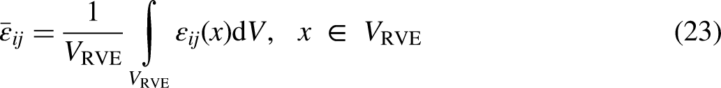
The homogenised macroscale constitutive behaviour of a 3D composite with reinforcement can be described as:

$${\overline{\sigma }}_{ij}={\overline{C}}_{ijkl}{\overline{\epsilon }}_{ij}i,j,k,l=1,2,3$$

(24)

The necessary condition for the equivalence between the heterogeneous composite medium and the homogeneous composite medium, as expressed in equation (24), is known as the Hill condition ³⁴ :

$${\displaystyle \frac{1}{2}\underset{V_{\mathrm{RVE}}}{\int }{\sigma }_i{\epsilon }_i\mathrm{d}V={\displaystyle \frac{V_{\mathrm{RVE}}}{2}\overline{{\sigma }_i}.\overline{{\epsilon }_i}i=1,2,\dots ,6}}$$

(25)

This ensures that the strain energy between the homogeneous and heterogeneous media is equivalent. Equation (24) defines the elastic properties from an elastic point of view.

Periodic boundary conditions

To determine homogenized mechanical properties such as Young's modulus, periodic boundary conditions (PBCs) were applied to the RVEs. PBCs simulate a structure as an infinite system by ensuring identical deformation across opposite boundaries, effectively eliminating boundary or edge effects. While real materials have boundaries and experience edge effects, a finite system with numerous repeating units behaves similarly to an infinite one as discussed in the ‘Finite element analysis’ section. This assumption is based on the premise that in a system with many repeating units, the proportion of boundary units to internal units is small. Consequently, the overall deformation behaviour and mechanical properties of the system are primarily determined by the deformation of the internal units that constitute the bulk material. This method is particularly useful for studying structures with large periodic patterned systems which can be represented by RVEs, as it minimizes computational resources and time. ³⁵

The strain fields within heterogeneous materials are broken down into two components: a microscale contribution denoted as ${\epsilon }_{ij}^{\mathrm{\prime }}$ ( $x$ ), and a macroscale contribution represented by ${\overline{\epsilon }}_{ij}$ . The overall strain field can be expressed as ³³ :

$${\epsilon }_{ij}(\mathit{x})={\overline{\epsilon }}_{ij}+{\epsilon }_{ij}^{\mathrm{\prime }}(\mathit{x})$$

(26)

The microscopic fluctuation, ${\epsilon }_{ij}^{\mathrm{\prime }}$ ( $x$ ), arises from the presence of a second phase such as fibres or particles at the local scale. When analysing a structure obtained by periodically replicating an RVE in space, the displacement field can be expressed as ³⁶ :

$$u_i={\epsilon }_{ij}^0{x}_j+{\nu }_i,\mathit{x}\in V_{\mathrm{RVE}}$$

(27)

In the context of an RVE, ${\epsilon }_{ij}^0$ represents a predefined strain field. The dimension of the RVE is denoted by L, and the displacement fluctuation $\mathit{v}$ exhibits periodicity over this length. Consequently, the displacement fluctuation at one boundary ( ${\nu }_1{\mid }_{x=0}$ ) is equal to that at the opposite boundary ( ${\nu }_1{\mid }_{x=L}$ ). The boundary condition for displacement is expressed as

$$u_i{\mid }_{x=L_j}=u_i{\mid }_{x=0}+{\epsilon }_{ij}^0{L}_j$$

(28)

The implementation of periodic boundary conditions gives:

$$\underset{V_{\mathrm{RVE}}}{\int }{\sigma }_{ij}{\nu }_{ij}\mathrm{d}V=0\mathrm{and}{\overline{\epsilon }}_{ij}={\epsilon }_{ij}^0$$

(29)

Which satisfies the Hill condition.

The periodic boundary conditions were applied using displacements and strains in ANSYS Mechanical. A schematic of the applied boundary conditions on a 2D and 3D geometry can be seen in Figure 3. For the 2D RVE, at X = 0, the X direction was fixed with the Y direction free, and at Y = 0 the Y direction was fixed with the X direction free. In addition, at Y = L the edge nodes were coupled using ANSYS mechanical remote points with only the Y direction active. This was to ensure that the edge at Y = L deforms the same as the edge at Y = 0. Finally, a strain of 3%, using displacements adjusted to match the appropriate length of the RVE, was applied to the edge at X = L to stay in the elastic region of the composite as constituent materials are defined as linear elastic. An applied tensile strain simulates real-world tensile testing of materials. The resulting force was determined using a force reaction probe applied to the face at X = L. This procedure was repeated by applying the strain at the Y = L face and coupling the nodes at the edge at X = L while the other boundary conditions remained the same. The modulus for the X and Y directions was calculated using equation (30) and averaged to obtain the final modulus value. A similar procedure was applied to the 3D RVE with the modulus in the X, Y, and Z directions being averaged to obtain the final modulus value.

$$E={\displaystyle \frac{\sigma }{\epsilon }={\displaystyle \frac{F/A}{\mathrm{\Delta }l/l}}}$$

(30)

Figure 3.

Schematic of the applied boundary conditions to a 2D and a 3D geometry.

where F, A, and $\mathrm{\Delta }l/l$ are the reaction force, cross-sectional area, and strain, respectively.

2D and 3D finite element modelling of nanocomposites

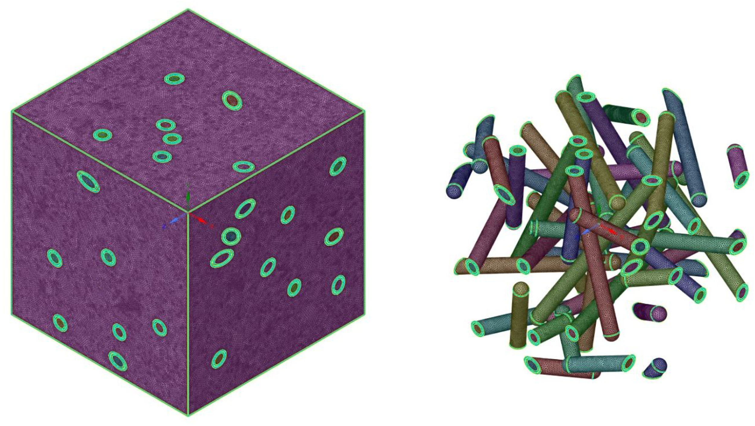
2D RVEs for nanocomposites were generated using Digimat-FE. The aspect ratio of nanofillers was set to 20, the inclusion shape to ellipsoid, the inclusion size to 500 nm, and the orientation to random 2D. Periodic geometry was employed without allowing interpenetration between the interphases and nanofillers. Enforcing periodic boundary conditions ensured that when the nanofillers were cut at one end of the RVE, they continued and entered the RVE at the parallel opposite surface. The interphase was modelled with a constant thickness around the nanofillers using the interphase thickness values obtained from the Ji model. Three random seeds produced unique RVEs for 2.5 wt% and 5 wt% particle loadings. These RVEs corresponded to different experimental treatments: untreated particles with and without interphase, and particles with 0.2 degree of substitution (DS) and 0.8 DS CNC esterification, which was represented by the inclusion of the interphase. Figure 4(a) shows the generated 1500 nm RVEs with 5 wt% particle loading and 0.2 DS esterification. The RVE geometries were then exported to ANSYS Mechanical, where periodic boundary conditions as described in the ‘Equivalent constitutive relation’ section were applied. A plane strain problem was defined, and material properties for the matrix, nanofillers, and interphase were obtained from the Ji equation and applied to the relevant geometries in the RVEs. The interphase Poisson's ratio was assumed to be equal to the matrix. The constituents of the RVE were assumed to be linearly elastic, isotropic materials with perfectly bonded contacts. A global conformal mesh of 15 nm with three steps of edge refinement was generated as shown in Figure 5(a). The number of elements ranged from 58,000 to 115,000 for 2.5 wt% and 5 wt% CNC particle loading, respectively. The moduli in X and Y directions were calculated for each RVE, and the calculated moduli were compared to experimental results.

Figure 4.

Three different RVEs obtained from three random seeds for 1500 nm 2D (a) and 500 nm 3D (b) geometries with matrix, 5 wt% CNC fillers, and interphases as they are labelled.

Figure 5.

Generated meshes and close ups for 1500 nm 2D geometry (a) and 500 nm 3D geometry (b) with 5 wt% CNC particles loading and interphases.

The random 3D RVE geometries were also created using Digimat-FE with an aspect ratio of 20, inclusion size of 500 nm, sphero-cylindrical inclusion shape, and random 3D orientation using periodic geometry without allowing interpenetration between nanofillers and interphase/nanofillers. Three random seeds produced unique RVEs for each of the experimental treatments: an untreated particle with and without Interphase, and an RVE with 0.2 DS and 0.8 DS CNC esterification at 2.5 wt% and 5 wt% CNC particle loadings. The generated 500 nm RVEs for 0.2 DS CNC esterification at 5 wt% CNC loading are shown in Figure 4(b). The geometries were then exported to ANSYS mechanical, and the periodic boundary conditions described in the ‘Equivalent constitutive relation’ section were applied. The procedure and assumptions about the material properties for the 2D RVEs were applied to the 3D RVEs. A 4-nm mesh with contact sizing of 2 nm between the matrix, interphase, and nanofillers was applied to the RVE to reduce computational cost seen in Figure 5(b). The number of elements for the 3D model ranged from 3,700,000 for 2.5 wt% CNC particle loading to 6,500,000 for 5 wt% CNC particle loading. The moduli in X, Y, and Z directions were calculated for each RVE and the results were compared to experimental results.

Results and discussion

Analytical models

The values of $E_{\mathrm{i}}$ and Y for the Ji model in equation (21) were unknown, so Python's optimisation library was used to determine them. The pseudo-code in List 1 provides an outline of the Python script used for this purpose:

List 1. Pseudo-code used for estimating the modulus of CNC/epoxy nanocomposite in the Ji model.

Algorithm Minimise

The experimental results were taken from Trinh and Mekonnen ⁸ for untreated and esterified treated CNC with DS of 0.2, 0.8, and 2.4 in an epoxy matrix, having a ±6% experimental variation for each observation. For the esterification modification, CNC was dispersed in toluene and homogenised. This dispersion was then heated to 90 °C, after which lauroyl chloride and pyridine were added. The reaction was carried out at 110 °C for 1 hour, followed by quenching with ethanol and washing with ethanol and acetone. The modified CNCs were characterized using FTIR spectroscopy, elemental analysis, X-ray diffraction, and contact angle measurements. For the preparation of epoxy biocomposites, epoxy resin was mixed with CNC, homogenized, degassed, and cured at 60 °C for 12 hours, followed by post-curing at 120 °C for 2 hours. They tested epoxy nanocomposites at 2.5 wt% and 5 wt% CNC loading and reported the elongation at break, tensile strength, and tensile modulus.

The data in Table 1 shows that CNC esterification treatment increased the thickness of the interphase as the improved bonding facilitated more adsorption points between polymer chains and the CNC particles. This resulted in more entanglement of polymer chains and CNCs and thicker interphases.

Table 1.

Calculated E_i, t, and Y for each nanofillers loading and CNC esterification treatment.

Matrix	Filler	Treatment	$E_{\mathrm{f}}$ (GPa)	$E_{\mathrm{m}}$ (GPa)	$E_{\mathrm{c}}$ (GPa)	$E_{\mathrm{r}}$ (GPa)	${\varphi }_{\mathrm{f}}$ (wt%)	d (nm)	l (nm)	t (nm)	$E_{\mathrm{i}}$ Takayanagi (GPa)	a	Y	$E_{\mathrm{i}}$ Ji (GPa)
Epoxy	None	NA	0	2.62	2.62	1.00	0.00	0.00	0.00	0.00	0.00	-	0.00	0.00
	CNC	None	140	2.62	3.30	1.26	0.025	0.03	0.50	8.39	8.57	-	0.12	13.77
			140	2.62	3.41	1.30	0.05	0.03	0.50	8.39	8.57	-	0.12	13.77
		0.2 DS esterification	140	2.62	3.57	1.36	0.025	0.03	0.50	12.37	10.60	-	0.39	36.44
			140	2.62	3.78	1.44	0.05	0.03	0.50	12.37	10.60	-	0.39	36.44
		0.8 DS esterification	140	2.62	3.41	1.30	0.025	0.03	0.50	10.83	9.83	-	0.27	26.38
			140	2.62	3.71	1.42	0.05	0.03	0.50	10.83	9.83	-	0.27	26.38
		2.4 DS esterification	140	2.62	2.31	0.88	0.025	0.03	0.50	1.19	1.80	1.83	0.76	9.75
			140	2.62	2.21	0.85	0.05	0.03	0.50	1.19	1.80	1.83	0.76	9.75

Considering the analytical models’ assumption that the CNCs are perfectly bonded with the epoxy matrix, there exists variation between the predicted and experimental results of the $E_{\mathrm{r}}$ , depicted in Figure 6(a) when unmodified CNCs are incorporated into the epoxy matrix. While both Ji and Takayanagi models with interphase fell within the experimental variations, the Ji model was closer to the average values. At 2.5 wt% CNCs loading, the Takayanagi model without interphase was outside of the experimental variation while at 5 wt% CNC loading it was within the experimental range. This shows the importance of including the interphase region in the modelling for accurate results.

Figure 6.

Comparison of the Takayanagi model and its modifications with experimental results for 2.5 wt% and 5 wt% particle loading with no CNC particle treatment (a), 0.2 DS esterified CNC (b), 0.8 DS esterified CNC (c), and 2.4 DS esterified CNC (d).

When CNCs were treated with 0.2 DS esterification, the bond between the CNCs and the epoxy matrix improved due to increased hydrophobicity. ⁸ This enhanced compatibility with non-polar polymer matrices leading to improved bonding. As a result, the assumption of perfect bonding in the analytical models become more valid. In this case, the Ji model was more accurate in the prediction of the $E_{\mathrm{r}}$ than the modified Takayanagi model. In addition, the modified Takayanagi model exceeded the experimental variation at 5 wt% CNC loading. The unmodified Takayanagi model failed to accurately predict $E_{\mathrm{r}}$ due to the absence of the interphase as shown in Figure 6(b).

When 0.8 DS CNC esterification is introduced, the $E_{\mathrm{r}}$ experienced a slight decrease compared to the 0.2 DS ester treatment, and both the Ji and modified Takayanagi models showed the variation depicted in Figure 6(c), but both were within the experimental range. This decrease can be attributed to higher degrees of esterification, which disrupted the crystalline structure of CNCs, resulting in a loss of inherent strength and stiffness. Furthermore, high levels of esterification hindered the CNCs’ ability to disperse effectively within the epoxy matrix. ⁸

When the CNC esterification level reached 2.4 DS, a negative impact on the $E_{\mathrm{r}}$ was observed. According to Trinh and Mekonnen, ⁸ the crystallinity of the CNC did not change significantly due to the 0.2 and 0.8 DS esterification treatments. However, the 2.4 DS treatment caused a significant reduction in crystallinity because the cellulose chains separated from their tightly packed crystalline structure resulting in an amorphous structure. This reduction in crystallinity caused a reduction in the modulus of the CNC particles. An additional variable representing the change in CNC modulus, $E_{\mathrm{f}}$ , was added to the minimisation algorithm in List 1 for the 2.4 DS esterification to account for this reduction in modulus. In addition, a variable to calculate aspect ratio ( $a$ ) was also added to the Takayanagi model. From Figure 6(d), both the Ji and Takayanagi models failed to accurately predict the reduction in $E_{\mathrm{r}}$ . Figure 7(b) showed that, for the Ji model, the minimisation algorithm initially kept the modulus of CNC constant and then reduced the Y value. Subsequently, it reduced the modulus of the CNC to the lower bound of 7.6 MPa and increased the Y value. One specific issue with the Ji model is that the ${\left(\frac{E_{\mathrm{r}}-1}{11}\right)}^{0.294}$ term, which governs the nonlinearities due to agglomeration, results in a complex number when $E_{\mathrm{r}}$ is less than 1. This is the case with the 2.4 DS esterification treatment for both 2.5 wt% and 5 wt%. The resulting complex number prevents the Ji model from predicting the reduction in $E_{\mathrm{r}}$ due to the 2.4 DS esterification modification as casting complex values to real ones discards the imaginary part. The results obtained from the analytical models demonstrate their inability to predict the nonlinearities associated with excessive fibre treatment.

Figure 7.

Comparison of the convergence of calculated E_r values (a) and Y and E_f values (b) from the minimisation algorithm used for the Ji model.

In conclusion, the Ji model was the most accurate analytical model for the untreated, and 0.2, and 0.8 DS esterification treated CNCs. The values obtained for the interphase thickness and modulus from the Ji model were used as input for the FEA models.

Finite element analysis

Verification of boundary conditions using material designer

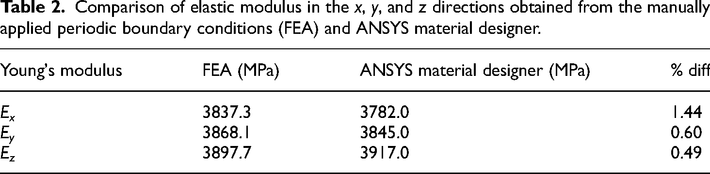
The accuracy of the periodic boundary conditions was verified by comparing the results from the manually applied periodic boundary conditions with the results from material designer module in ANSYS. The 500 nm RVE with 5 wt% CNC particles loading, and 0.2 DS CNC esterification was imported into material designer as a user defined geometry and material properties were applied to the relevant geometries. Conformal meshing with a maximum size of 4 nm that adapted towards the edges was applied to the RVE shown in Figure 8. The difference between the elastic modulus from both models in the X, Y, and Z directions was less than 1.5% as shown in Table 2, indicating that the manually applied boundary conditions were behaving as expected.

Figure 8.

Mesh of the imported geometry to ANSYS material designer with and without matrix visibility.

Table 2.

Comparison of elastic modulus in the x, y, and z directions obtained from the manually applied periodic boundary conditions (FEA) and ANSYS material designer.

Young's modulus	FEA (MPa)	ANSYS material designer (MPa)	% diff
Ex	3837.3	3782.0	1.44
Ey	3868.1	3845.0	0.60
Ez	3897.7	3917.0	0.49

Size of 2D and 3D RVE

Mesh sensitivity analyses for 2D and 3D models were conducted, and the results are presented in Figure 9. When the edge refinement was increased from 1 to 3 for the 2D geometry, the number of elements increased from 41,000 to 115,000, and the average von Mises stress converged to 286.6 MPa. A similar trend was observed for the 3D geometry when the contact mesh size was decreased from 10 nm to 2 nm. The edge refinement of level 3 was chosen for the 2D model because there was a negligible difference in solution time among the three edge refinements. The same applied to the 3D geometry with a 2 nm contact size.

Figure 9.

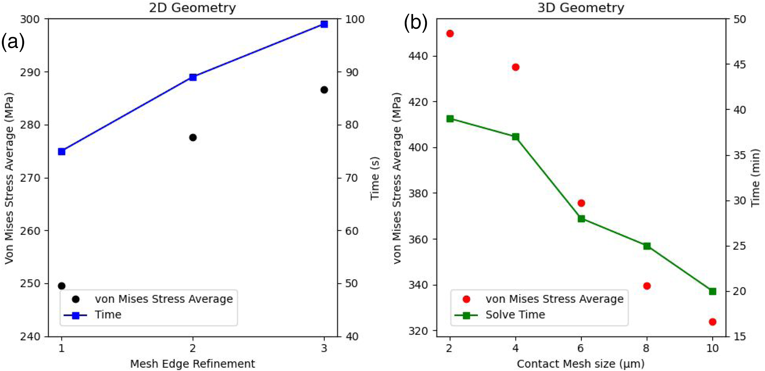
Mesh sensitivity analysis for 2D (a) and 3D (b) geometries, showing the increase in edge refinement for the 2D geometry and the contact mesh sizing for the 3D geometry. The solution time for both geometries is also presented.

2D RVEs with dimensions ranging from 2500 nm to 10,000 nm for 2.5 wt% CNC loading and 1000 nm to 1750 nm for 5 wt% CNC loading were generated using Digimat-FE for 0.2 DS CNC esterification treatment. The generated geometries for 5 wt% CNC loading are shown in Figure 10(a). RVEs of nanocomposite with 2.5 wt% CNC nanofillers loading exhibited a similar trend. For RVE with 2.5 wt% CNC loading to achieve results within the experimental variation, the minimum size of the RVE must be 7500 nm as shown in Figure 11(a). This result is expected as less fillers are present in the 2.5 wt% particle loading RVE, therefore a larger RVE is needed to be a statistical representation of the nanocomposite. Similarly, in Figure 11(b), the 1000 nm RVE, with 5 wt% CNC nanofillers loading, underestimated the experimental modulus, while the 1250 nm RVE overestimated it. This discrepancy arose because the smaller RVEs lacked sufficient nanofillers to be a statistically representative sample of the entire system. However, when the RVE size increased to 1500 nm, the difference between experimental and numerical results fell within the variation in the experimental data. At this size, there were enough nanofillers in the RVE to accurately represent the composite system at the macro level. Further increasing the RVE to 1750 nm showed negligible changes in the modulus, indicating convergence of the results. Consequently, the RVE with the size of 1500 nm was chosen for simulating both treated and untreated composites due to its lower computational cost compared to the RVE with the size of 1750 nm, while maintaining accuracy.

Figure 10.

Different sizes of RVE for 0.2 DS CNC esterification treated 5 wt% particle loading in 2D (a) and 5 wt% particle loading in 3D (b) FEA models with interphase.

Figure 11.

Variation of Young’s modulus versus RVE size for 2D and 3D FEA models for 0.2 DS CNC esterified particles.

Similarly, four different sizes of 3D RVEs with 5 wt% CNC particle loading, with 0.2 DS CNC esterification treatment, were modelled using Digimat-FE and simulated in ANSYS Mechanical. The sizes of RVEs ranged from 250 nm to 625 nm as shown in Figure 10(b). As seen in Figure 11(c), the smaller RVEs lacked sufficient nanofillers to be statistically representative of the macro-scale system, resulting in either overestimated or underestimated elastic modulus. The different sizes of the RVE for 5 wt% CNC particle loadings are shown in Figure 10. Figure 11(d) shows that the results converged when the RVE size increased from 500 to 625 nm. Consequently, the optimal RVE size for the 5 wt% CNC particle loading was determined to be 500 nm, striking a balance between computational cost and accuracy. In the 500 nm RVE, there were sufficient nanofillers resulting in a homogenised material model. However, the 250 nm and 375 nm RVEs could not accurately predict the modulus. For the 2.5 wt% CNC particle loading, an RVE of 750 nm was necessary to accurately represent the modulus.

At smaller sizes, the RVEs in Figure 11(b) and (c) exhibited large fluctuations in elastic modulus. This was due to the size of the RVE not capturing proper distributions of the 500 nm particles. Consequently, anisotropic behaviour was observed, with high values of elastic moduli in one direction increasing the average elastic modulus. As the size of the RVE increased above 500 nm, the particle distribution became more representative of the macro model, causing the RVE to behave in an isotropic manner with less fluctuations in the values.

Comparison of 2D and 3D FEA models

Table 3 compares the experimental elastic modulus results to the elastic modulus calculated from the 2D and 3D finite element analysis. In the case of the untreated composite, incorporating an interphase into the 3D FEA model led to improved accuracy in the results. For the 2.5 wt% CNC particle loading nanocomposite, the difference decreased from 5.3% to 0.8%, bringing the value closer to the experimental modulus. When the volume fraction was increased to 5 wt% CNC particle loading, the difference reduced from 3.3% to 1.2% with the addition of the interphase, although both values were within the experimental variation. For the 2D FEA model, at 2.5 wt% CNC particle loading both models with and without the interphase were within the experimental variation. However, at 5 wt% CNC particle loading, both models overestimated the elastic modulus and exceeded the experimental range. Therefore, for untreated PNC, 3D FEA models are more accurate as they consider the interactions between the nanofillers better than the 2D models. Also, as discussed in the ‘Analytical methods’ section, untreated nanofillers are not perfectly bonded to the matrix which explains the discrepancy between the experimental and the FEA results.

Table 3.

Comparison of elastic modulus from experiment and FEA results, including the standard deviations between the x and y components for the treated and untreated particles. The table also includes the standard deviation between the x and y components for each treatment of nanofillers.

	Treatment	Interphase	wt%	FEA (MPa)	Experiment (MPa)	Difference (%)	STDEVx (%)	STDEVy (%)	STDEVz (%)	STDEVxy (%)	STDEVxyz (%)
2D	No treatment	No	2.5	3134	3300	5.03	5.93	4.34	-	1.01	-
			5	3681	3414	7.82	0.80	3.15	-	3.62	-
		Yes	2.5	3241	3300	1.80	1.04	1.03	-	1.16	-
			5	3660	3414	7.21	0.80	3.15	-	4.62	-
	0.2 DS ester	No	2.5	3134	3569	12.19	5.93	4.34	-	1.01	-
			5	3611	3780	4.46	0.80	3.15	-	3.62	-
		Yes	2.5	3355	3569	6.01	1.21	0.78	-	1.21	-
			5	3833	3780	1.41	0.59	5.11	-	5.59	-
	0.8 DS ester	No	2.5	3134	3414	8.20	5.93	4.34	-	1.01	-
			5	3611	3714	2.77	0.80	3.15	-	3.62	-
		Yes	2.5	3257	3414	4.58	1.05	1.02	-	1.18	-
			5	3766	3714	1.39	2.36	3.25	-	3.30	-
3D	No treatment	No	2.5	3124	3300	5.33	6.91	2.28	7.90	-	4.97
			5	3303	3414	3.25	3.13	2.12	5.05	-	6.16
		Yes	2.5	3274	3300	0.80	3.09	5.28	8.24	-	4.09
			5	3454	3414	1.19	3.13	2.12	5.05	-	2.52
	0.2 DS ester	No	2.5	3124	3569	12.47	6.91	2.28	7.90	-	4.97
			5	3303	3780	12.62	3.13	2.12	5.05	-	6.16
		Yes	2.5	3380	3569	5.29	3.64	3.19	0.84	-	2.05
			5	3741	3780	1.02	3.20	3.86	2.99	-	2.91
	0.8 DS ester	No	2.5	3124	3414	8.49	6.91	2.28	7.90	-	4.97
			5	3303	3714	11.07	3.13	2.12	5.05	-	6.16
		Yes	2.5	3312	3414	3.00	1.00	0.90	1.01	-	0.92
			5	3753	3714	1.07	4.09	3.97	2.22	-	2.49

When the treatment of nanofillers was considered in the modelling, the 2D and 3D FEA models encountered challenges in making accurate predictions without the inclusion of the interphase. Specifically, for the 0.2 DS CNC ester treated 2.5 wt% CNC particle loading nanocomposite, the discrepancy of the calculated elastic modulus from the experimental results was reduced from 12.5% to 5.3% upon the inclusion of the interphase in the 3D RVE models and it was reduced from 12.2% to 6.0% for 2D RVE models. A similar improvement was observed for 5 wt% CNC particle loading when the discrepancies reduced from 12.6% and 4.5% to 1.4% and 1.0% for 3D and 2D RVEs models, respectively. According to the Ji analytical model, the esterification treatment of CNCs led to an increase in the thickness and modulus of the interphase. These increases resulted in the models incorporating the interphase to accurately predict the modulus of the PNC. For RVEs without the interphase, the increase in the thickness and modulus of the interphase cannot be simulated as they lack the geometries representing the treatment. Nevertheless, the 5 wt% CNC particle loading 2D RVE without the interphase fell within the experimental variation due to the presumption of perfect bonding between the nanofillers and the matrix. The esterification enhanced this bonding, as discussed in the ‘Analytical methods’ section. A similar trend was seen for 0.8 DS CNC esterification treatment. In general, the 3D RVEs were more accurate than the 2D RVEs, however, for predicting the modulus for treated CNC, 2D geometries offer sufficient accuracy at a fraction of the computational cost and time.

Table 3 also contains the standard deviations, represented by STDEVx, STDEVy, and STDEVz, of the calculated directional elastic modulus between the three different generated 3D RVEs. These values were obtained when the uniaxial strain was applied individually in the X, Y, and Z directions. The deviations were all below 6% indicating that there were no significant differences between each of the directional moduli for the different generated 3D RVEs. Thus, the method used to generate the 3D RVEs was able to capture the elastic behaviour of the nanocomposites accurately without significant deviation irrespective of the loading direction. STDEVxyz in Table 3 represents the standard deviation among the modulus in X, Y, and Z directions for each of the individually generated 3D RVEs. The deviation was less than 5% indicating that the material behaved in an isotropic manner. When short CNC particles are uniformly distributed within a matrix, their random orientation in three dimensions ensures that they are not preferentially aligned in any specific direction. Consequently, the material behaves as an isotopic material. If the particles are randomly distributed concerning both orientation and position, samples of the material containing statistically significant numbers of particles tend to exhibit isotropic behaviour, meaning the material behaves in a similar manner in all directions due to the random arrangement of particles.^37,38 Babu et al. ³⁷ found that completely random 3D orientation of microscopic short fibres behaves like an isotropic material at the macroscale. They simulated five different RVEs with different distributions of fibres and found that the values of elastic modulus, shear modulus and Poisson's ratio obtained in the X, Y, and Z directions only differed by 4%. The values obtained in our study varied by less than 6% which is within the experimental variation. Zhao et al. ³⁸ also observed similar behaviour for short fibres that are randomly distributed.

Overall, for the 2D RVEs, the standard deviations remained below 4%, indicating the efficacy of the method used to generate the RVEs. The standard deviation in 3D RVEs models did not exceed 6 experimental range, indicating that the 3D RVEs also exhibited isotropic behaviour.

2D and 3D stress fields

Figure 12 compares von Mises stress contour plots obtained when the strain was applied in the X and Y directions to the 5 wt% CNC particles loading 2D RVEs and Figure 13 compares von Mises stress contour plots obtained when the strain was applied in the X, Y and Z directions to the 5 wt% CNC particles loading 3D RVEs models. The stresses were distributed throughout the PNC with the highest stresses concentrated around the ends of the nanofillers between the nanofiller/interphase interfaces. Compared to the matrix, the fillers and interphase experienced higher stresses, confirming their reinforcing effect. The stresses present in the nanofillers, and the matrix remain below their respective yield strength, confirming that the applied strain was within the elastic region of the PNC. Additionally, the difference in stresses between all the directions is less than 3%, indicating isotropy in the RVEs.

Figure 12.

2D von-Mises equivalent stress when strain was applied in the X (a) and Y (b) direction showing a close up view of the area with the highest stress concentration.

Figure 13.

3D von-Mises equivalent stress when the strain was applied in the X (a), Y (b) and Z (c) direction. Ai, Bi, and Ci shows the RVE with the matrix, nanofiller and interphase. Aii, Bii, and Cii shows the nanofiller only and Aiii, Biii, and Ciii shows the interphase only.

In practice, the 2D RVEs can be used for their computational efficiency; however, they may not capture local stress and strain distributions as accurately as 3D RVEs. The 3D RVEs offer a more precise representation of the material's microstructure, making them essential for detailed local analysis, but at a higher computational cost. The choice between 2D and 3D RVEs depends on the specific requirements of the simulation. If the goal is to understand the overall material behaviour under certain loading conditions, 2D RVEs offer sufficient accuracy at a fraction of the computational cost of 3D RVEs. However, for applications requiring detailed insights into local phenomena like crack propagation and initiation, 3D RVEs are more appropriate. Another option is to use a hybrid approach where 2D RVEs are used for preliminary analysis and 3D RVEs for detailed studies which would balance the accuracy and speed of simulations.

Comparison of analytical and FEA models

Figure 14 compares the ${\mathrm{E}}_{\mathrm{r}}$ values derived from both analytical and FEA models. The untreated nanofillers’ outcomes are depicted in Figure 14(a). At 2.5 wt% CNC nanofillers loading, the results from all models, except for the Takayanagi model without interphase, fell within the experimental variation. However, as the CNC nanofillers loading increased to 5 wt%, the 2D FEA models overestimated the PNC relative modulus and it fell outside the experimental range. The 3D FEA model demonstrated superior accuracy at both 2.5 wt% and 5 wt% CNC nanofillers loadings, attributable to its ability to simulate intricate interactions among the nanofillers, interphase, and matrix.

Figure 14.

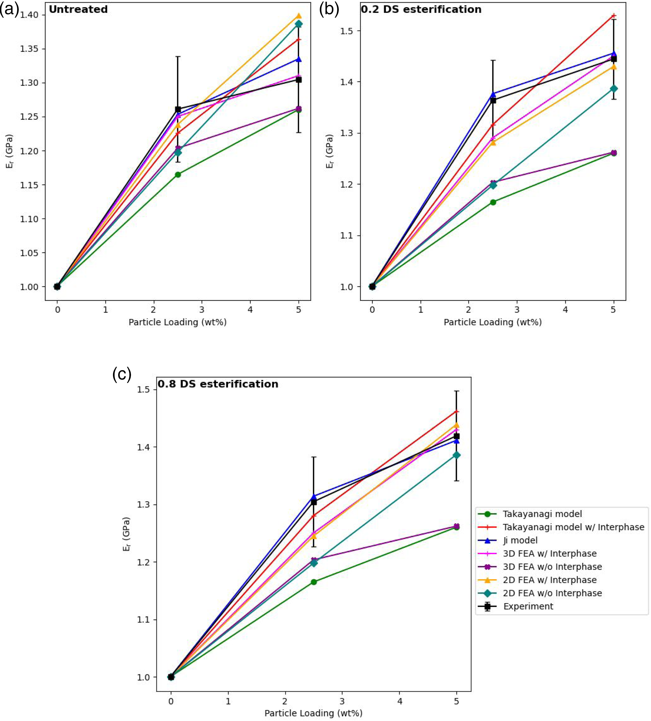
Comparison of elastic moduli values obtained from analytical, 2D and 3D FEA models for untreated nanofillers (a), 0.2 DS esterified CNC nanofillers (b) and 0.8 DS esterified CNC nanofillers (c).

Figure 14(b) illustrates the ${\mathrm{E}}_{\mathrm{r}}$ values for 0.2 DS CNC esterification. The 3D and analytical models, in the absence of interphase, underestimated the modulus, whereas, for the 5 wt% CNC particle loading, the 2D model without the interphase yielded acceptable results. The Ji model exhibited optimal performance at 2.5 wt% CNC particle loading, and the 3D model with interphase was the most accurate at 5 wt% CNC particle loading. The Ji analytical model assumed agglomeration, which was not modelled in the FEA models in this work, resulting in the analytical model's superior accuracy at 2.5 wt% CNC particle loading.

A similar trend is observable for the nanofillers treated with 0.8 DS CNC esterification shown in Figure 14(c).

To increase the accuracy at 2.5wt% loading for the 2D and 3D model so that it would be on par with the Ji model would involve simulating a larger RVE. As discussed in the ‘Size of RVE’ section the RVE must be statistically representative of the whole medium. At lower particle loading, a larger RVE is needed to capture the properties of the whole medium. However, increasing the size of the RVE too much would prohibitively increase the computational cost. In addition, in practice, every CNC would not be evenly distributed in the epoxy matrix. Therefore, modelling agglomerates in the RVE can increase accuracy. However, since the modulus increased from 2.5 wt% to 5 wt% it was assumed that agglomeration was negligible and not modelled in this paper.

To increase the accuracy at 5 wt% loading for the Ji model for it to be closer to the 3D FEA model, modifications of the equation are needed. From equation (14), the Ji model made a simplification for the shape of the nanoparticles. If the equation for the shape of the CNC was used in the Ji model, then the accuracy may improve and be closer to the 3D model at 5 wt% loading. However, modifying the existing analytical models was outside the scope of this project. In addition, using more powerful optimization algorithms, other than Python's minimization, can further increase accuracy at the 5 wt% loading condition. However, more powerful optimization techniques would be incompatible with the simple Takayanagi and Ji models and thus would need to be modified which was outside the scope of this paper. These more powerful optimization algorithms can however be used on the FEA methods which will be discussed in the next section.

Parametric analysis

Since the analytical models failed to accurately predict the $E_{\mathrm{r}}$ values for the 2.4 DS esterification treatment, their values for interphase modulus and thickness were not used. Instead, the design of experiments (DOE) with ANSYS response surface optimisation was used to find the optimal interphase thickness and modulus as well as the modulus of CNC after the crystallinity reduction due to 2.4 DS esterification. It works by first creating a set of experiments through the DoE method, which systematically varies the input parameters to understand how changes affect the outputs. Using the results from these experiments, a mathematical model called the response surface is generated. This model approximates the system's behaviour and predicts output responses based on the input parameters. The response surface is then used to find the optimal set of input parameters that achieve the desired output, considering objectives like minimizing or maximizing the modulus. ³⁹

Since it was established in Table 3 that different random distributions of the RVE and the $E_{\mathrm{r}}$ obtained from the X, Y, and Z directions are statistically the same, only one RVE with a set random particle distribution and force applied in the X direction was used for the parametric analysis. Parametric analysis was performed on 2D geometries as they were found to be sufficiently accurate with much lower simulation time compared to 3D geometries.

ANSYS Response Surface optimisation was used with Latin hypercube sampling (LHS) (n = 10) and user defined results to explore the design space. LHS was chosen because it helps explore the design space with a smaller number of samples and reduces spurious dependencies compared to completely random Monte Carlo methods. Since the imported geometry from DIGIMAT-FE could not be parameterized in ANSYS, 30 different RVEs with interphase thicknesses ranging from 0 nm to 12 nm and aspect ratios of CNC ranging from 5 to 20 were generated. These sizes of the interphase were selected to optimize computational costs and minimize meshing errors. An interphase thickness below 3 nm prohibitively increases the computational time and the likelihood of meshing errors. Due to the presence of excess fatty acids for 2.4 DS esterification, it can be assumed that the interphase would be larger than the 0.8 DS treatment. There are several different reported values for interphase thickness including a few nanometres, ¹³ half the diameter of the particle, ⁴⁰ or 0.5 to 3.25 times the diameter. ⁴¹ As stated earlier, the excessive 2.4 DS esterification caused delamination of the crystalline cellulose structure. Therefore, it can be assumed that swelling of the nanocellulose would occur and the aspect ratio would decrease. Due to the increased diameter due to swelling, the interphase would increase according to Qiao et al.. ⁴¹

Since no reinforcement effect was observed for the 2.4 DS esterified composites, it was assumed that the modulus of the CNC was below that of the epoxy matrix (2.62 GPa). Therefore, the upper and lower bounds of the LHS search were set at 2.62 GPa and 0 GPa, respectively. Similarly, the modulus of the interphase must lie between that of the CNC and the matrix. Consequently, the same upper and lower limits were applied to the modulus of the interphase.

After the design space was explored, the ANSYS optimisation module was used to determine the optimum CNC modulus and interphase modulus, and thickness to obtain results closer to the experiment. Ansys includes the option for three different optimisation algorithms, namely Multi-Objective Genetic Algorithm (MOGA), Non-Linear Programming by Quadratic Lagrangian (NLPQL), and Mixed-Integer Sequential Quadratic Programming (MISQP). MOGA was chosen as it is ideal for problems where multiple material properties need to be optimised simultaneously as is the case with the 2.4 DS esterification process. MOGA works by finding a set of optimal solutions known as the Pareto front, where no single solution is superior to another across all objectives. The process begins with the initialisation of a randomly generated population of solutions that are evaluated based on how well they meet the multiple objectives resulting in a vector of values. Selection methods such as ranked-based selection are used to choose solutions for the next generation. This process continues until the desired interphase thickness and modulus and CNC aspect ratio are met. ⁴² MOGA with 9600 evaluations was used. MOGA is a type of algorithm that is used to solve problems with multiple objectives. The constraints were as follows: The interphase modulus and CNC modulus were set to minimize their values with a target of 1 Pa. For 2.5 wt% particle loading geometries, the variables were set to seek a target for force reaction of 519 N with upper and lower bounds of 550 N and 488 N, respectively. For the 5 wt% particle loading geometry, the variables were set to seek a target for a force reaction of 99.5 N with upper and lower bounds of 10.5 N and 93.5 N, respectively. These values corresponded to the upper and lower experimental bounds.

The interphase and nanocellulose moduli were varied, and the relative modulus of the different geometries was determined. The optimization found that the geometry with a 6 nm interphase thickness, an aspect ratio of 10, a CNC modulus of 1000 Pa, and an interphase modulus of 0.65 GPa was the most optimal. Figures 15(a) and 14(b) show the convergence of ANSYS’ optimization process of the relative modulus for 2.5 wt% and 5 wt%, respectively.

Figure 15.

Convergence of relative modulus from ANSYS optimisation process for 2.5 wt% (a) and for 5 wt% (b) in 2D models. Surface plot of interphase thickness against CNC aspect ratio with the resulting $E_{\mathrm{r}}$ for 2.5 wt% and 5 wt% in 2D geometries (c). Comparison of relative elastic moduli values obtained from analytical, 2D, and 3D FEA models for 2.4 DS esterified CNC nanofillers (d).

The response surface in Figure 15(c) represents the surface plot of interphase thickness and aspect ratio at the optimised interphase and CNC modulus of 0.65 GPa and 1000 Pa, respectively. It shows that when the aspect ratio was below 10 and the interphase thickness was larger than 6 nm, the calculated relative modulus was below the experimental value. The inverse relationship is also true. Since the interphase modulus was lower than the modulus value of the matrix, an increase in interphase thickness lowered the $E_{\mathrm{r}}$ of the composite as the higher modulus matrix was replaced with the lower modulus interphase. The same behaviour was observed when the aspect ratio of the CNC particles was lowered.

Figure 15(d) compares the $E_{\mathrm{r}}$ values calculated from the analytical and 2D and 3D models for the 2.4 DS esterified composites. The analytical models failed to accurately predict the reduction in $E_{\mathrm{r}}$ . However, when the optimised geometry and material properties mentioned earlier were added to the 2D model, the 5 wt% fell within the experimental range. The 3D geometry further improved the accuracy of prediction of the $E_{\mathrm{r}}$ . This was because the 3D geometry being able to capture the intricate interactions among the nanofillers, interphase, and matrix. It must be noted that the RVEs for the 2.5wt% and 5wt% for the 3D models were increased by 50 nm for them to be statistically representative of the entire medium.

Figure 16(a) and (b) represents the von Mises stress contour plots obtained when the optimised values were added to the 3D and 2D models. The stresses on the CNC were significantly lower than those in the matrix and interphase. This large disparity is due to stress concentration, which weakens the nanocellulose composite and could potentially lead to failure. In addition, the load-bearing area was reduced, resulting in a smaller area to support the applied forces, which further decreased the overall strength of the material. ⁴³

Figure 16.

3D (a) and 2D (b) von Mises equivalent stress contour plots when the strain was applied in the X direction.

Conclusion

In this study, statistical representations of a nanocomposite were developed using FEA modelling of 2D and 3D RVEs, along with analytical models, to infer the interphase properties and predict the elastic behaviour of esterified nanocellulose/epoxy bio-nanocomposites. FEA models, both with and without the interphase region, were analysed, and the accuracy of their predictions was assessed by comparing the results with experimental data.

Experimental studies have shown that esterification treatment of CNCs increases both the thickness and modulus of the interphase. Our findings show that incorporating the interphase into FEA models allows precise prediction of the PNC's behaviour. In contrast, RVEs without the interphase fail to accurately represent the treatment's effects, leading to underestimation of the material's modulus in both 3D FEA and analytical models.

Finite element analysis using RVEs with periodic geometry and boundary conditions has proven to be an effective method for homogenization. The elastic moduli from FEA RVE models incorporating the interphase generally aligned with experimental data. In addition, the random distribution and orientation of particles in these models led to isotropic behaviour. The Ji model performed best at 2.5 wt% CNC particle loading, while the 3D model with an interphase was most accurate at 5 wt%. The Ji analytical model, which accounted for agglomeration, achieved superior accuracy at 2.5 wt% particle loading, a factor not accounted for in the FEA models. Finally, 2D RVEs provided sufficient accuracy with significantly shorter simulation times compared to 3D RVEs.

The analytical models predicted inaccurate values of the elastic modulus for the 2.4 DS esterification treatment of CNCs. To address this, we used Design of Experiments (DoE) with ANSYS response surface optimization, determining the optimal interphase thickness, modulus, CNC modulus, and aspect ratio post-crystallinity reduction. Latin hypercube sampling (LHS) identified an optimal geometry with a 6 nm interphase thickness, an aspect ratio of 10, a CNC modulus of 1000 Pa, and an interphase modulus of 0.65 GPa. The response surface analysis showed that an aspect ratio below 10 or an interphase thickness above 6 nm resulted in a lower modulus than experimental values. The optimized 3D model accurately captured the interactions between nanofillers, interphase, and matrix, with stress contour plots revealing stress concentrations around the CNC particles, indicating potential weaknesses in the nanocomposite due to reduced load-bearing areas.