Sage Journals: Discover world-class research

Abstract

This study presents a novel approach to accurately predict the settlement of shallow foundations using advanced machine learning techniques while assessing the influence of key variables. Four machine learning models Gradient Boosting (GB), Random Forest (RF), Support Vector Machine (SVM), and K-Nearest Neighbor (KNN) are enhanced with Particle Swarm Optimization (PSO) for hyperparameter tuning, resulting in hybrid models GB-PSO, RF-PSO, SVM-PSO, and KNN-PSO. The experimental dataset comprises 189 samples, and model performance is rigorously evaluated through K-Fold Cross-Validation alongside R², RMSE, MAE, and MAPE metrics. The results indicate that PSO tuning does not consistently improve the prediction accuracy, with the original models, particularly GB and RF, outperforming their PSO-optimized counterparts. Sensitivity analysis via Shapley Additive Explanation (SHAP) highlights average Standard Penetration Test blow count (SPT) and footing width (B) as the most influential variables, with footing embedment ratio (D_f/B) and net applied pressure (q) also significantly impacting settlement predictions. The study offers a new Excel tool based on the GB model, facilitating practical applications for civil engineers, and providing a dependable, user-friendly tool to predict shallow foundation settlement.

Keywords

Machine learning settlement of shallow foundation average SPT blow count footing width b shapley additive explanation prediction

Highlights

Gradient Boosting achieves the highest accuracy (R² = 0.9484), making it the best model for shallow foundation settlement predictions.

Average SPT blow count negatively impacts settlement, while footing width B shows a strong opposing effect.

An Excel tool based on the Gradient Boosting model enables accurate settlement estimations within specified input ranges.

Introduction

For centuries, humanity has progressed continuously, shaping the course of history right up to the present day. Looking back to the earliest days, we find something not only ordinary yet special, but deeply familiar and comforting home. Homes are fundamental, not just for humans but for all species as they organize their environments. Birds build nests, snakes dig burrows, monkeys gather in trees, lions take shelter in caves or shade, and fish gather in underwater caves. Yet humans have taken this concept further, mastering the art of building and continuously enhancing the comfort, convenience, and functionality of their homes and buildings. A crucial element in construction is the foundation — it supports the full weight of a house, building, factory, or school. Designing a foundation requires attention to architectural form, intended function, structural integrity, and environmental factors to provide an optimal solution. Every project has its own unique characteristics, presenting challenges for design engineers, especially in the fields of structural and geotechnical engineering. This complexity has inspired ongoing research, as scientists and engineers seek to address these challenges and develop innovative solutions in foundation design and construction.

Small and medium-sized civil and industrial constructions now often choose shallow foundation solutions to save costs. This solution has a fast construction time, simple design, and construction to reduce costs compared to other methods. During construction and use, the settlement of the foundation directly affects the safety of the work. Karl Terzaghi proposed the theory of permeable consolidation and the principle of effective stress in 1923. On this basis, the research on the calculation theory of foundation settlement has made great progress. There are many methods to study the settlement of the ground layer, which can be basically divided into class sum method, finite element method, calculation method, empirical inference method, and combined prediction method.^1,2,3,4 The settlement of the foundation is influenced by many factors such as the magnitude and distribution of loads acting on the building, geological conditions, and the bearing structure system.^5,6,7 The weight applied on a foundation affects how much the soil beneath it will compress. When loads are concentrated or unevenly distributed, they can cause differential settlement, leading to structural stresses. Larger buildings, particularly those with asymmetrical designs or load concentrations, are more susceptible to these impacts.⁸ Soil type and condition play critical roles. For example, clay soils are more compressible than sandy soils, which results in greater settlement. The soil's elastic modulus (ability to return to original shape after compression) and cohesion properties (how well soil particles bind together) also determine settlement rates.⁹ The shape and size of a foundation's footing influence settlement characteristics.¹⁰ For instance, wider footings distribute loads over larger areas, reducing settlement. In addition, the presence of tie beams can help reduce differential settlement across multi-column structures, mitigating irregular displacement risks under varied soil conditions. Depth of water table can impact soil density and strength, with higher water tables leading to soil softening and increased settlement.¹¹ These factors underscore the complexity of predicting shallow foundation settlement, and recent models often integrate multiple variables to improve accuracy. This requires different methods complex calculation and analysis methods to be able to assess in detail and quantify risks for the project. On the basis of the settlement experiments, this study builds machine learning (ML) models, a more advanced and modern calculation method, to perform data simulation analysis to find an effective predictive model. The rapid advancements in artificial intelligence (AI) and machine learning (ML) technologies have led to notable progress in geotechnical reliability analysis, enhancing both computational precision and efficiency. Numerous researchers have contributed to this field, resulting in successful applications across various geotechnical contexts.¹²

The investigation of Wang et al.¹³ introduced a machine learning (ML) and multi-objective optimization (MOO) approach for enhancing the compressive strength and chloride ion resistance of Recycled Aggregate Concrete (RAC) while minimizing its environmental impact (EI) and life cycle costs (LCC). A database of 807 experimental samples was used to compare the performance of various ML models and swarm intelligence (SI) algorithms. The ML model Whale optimization algorithm- Back propagation neural network (WOA-BPNN) demonstrated the best predictive accuracy for compressive strength and electric charge passed, with R² values of 0.9904 and 0.9837 on the test set, respectively. SHAP and partial dependence plot (PDP) analyses identified cement, water, and curing age as key factors affecting RAC performance. The MOO model balanced compressive strength, electric charge passed, EI, and LCC, with fly ash being the most effective supplementary material to improve the RAC performance without increasing environmental or cost burdens.

In the construction industry, concrete poses major sustainability challenges, particularly due to cement production's environmental impacts. Replacing natural materials with recycled components, such as from construction and demolition waste (CDW), provides low-carbon potential. However, traditional models based on linear regression fall short in evaluating the performance of such complex material systems. Artificial intelligence (AI), with its nonlinear processing capabilities, offers a solution to model the intricate interactions in sustainable concrete. The reviewed studies of Wang et al.¹⁴ show that AI models, when coupled with comprehensive datasets that account for material composition and curing conditions, can optimize concrete mixtures and predict performance effectively, addressing the limitations of traditional approaches.

Literature review

Differences investigation using Machine Learning approaches have been used for predicting the settlement of the foundation. The method of predicting foundation settlement also moves from traditional prediction to prediction by algorithms, such as Artificial Neural Network (ANN),¹⁵ Adaptive neuro Fuzzy Inference System (ANFIS),¹⁶ Support vector machines (SVM),^17,18 and Genetic Programming (GP)^19,20 in order to get good results. Moreover, optimization algorithms such as Simulated Annealing (SA), and Particle Swarm Optimization (PSO) are used to create hybrid models in order to tune hyperparameters of Machine learning algorithms. Zhibin et al.²¹ proposed a PSO-optimized SVM model for predicting the foundation settlement. Jing Zhai¹⁸ used SVM, and the autoregressive model based on artificial bee colony optimization used to predict the foundation settlement reported significantly improved results compared to the single SVM model.

Table 1 summarizes some studies applying machine learning models to predict the settlement of shallow foundations. The above studies have shown that the application of machine learning to predict the settlement of shallow foundations has certain accuracy and reliability. Using an evolutionary artificial intelligence approach, Raja et Shukla²⁵ developed a hybrid ML model to predict the settlement of geosynthetic-reinforced soil foundations. Erzin and Gul²⁴ used the database containing 22 samples derived from the empirical formulation of Meyerhof²⁶ Terzaghi and Peck,²⁷ Parry,²⁸ Peck et al.,²⁹ and Burland and Burbidge³⁰ to develop an ANN model to predict the settlement of foundation from six input variables, such as footing geometry length L and width B, the footing embedment depth D_f, the bulk unit weight of the cohesionless soil γ, the footing applied pressure q, and corrected standard penetration test varied during the settlement analyses N_cor. Therefore, the practicality of the proposed ANN model of Erzin and Gul²⁴ seems to be improved. Thereby, Shahin et al.,²² Rezania and Javadi,²³ and Mohammed et al.¹⁶ attempted to develop ML models including ANN, GP and hybrid model ANFIS-PSO to predict the settlement of foundation from the real in situ data. These investigations have not quantified and evaluated the input variable effect on the settlement of the foundation. Moreover, one of the most critics of ML models is to be considered as the “black-box” model.

Table 1.

Application of artificial intelligence in settlement estimation.

Reference	Data	Method	Performance measures
Shahin et al.²²	187	ANN	R²= 0.820, RMSE = 11.04, MAE = 8.78
Rezania and Javadi²³	173	GP	R²= 0.826, RMSE = 11.07, MAE = 6.77
Erzin and Gul²⁴	22	ANN	R²= 0.990, RMSE = 1.79, MAE = 1.30
Mohammed et al.¹⁶	188	ANFIS-PSO	R²= 0.8650, RMSE = 9.02, MAE = 6.50

In the study of Friedman³¹ introducing GB, explained that the algorithm builds models on the residuals of data, reducing the impact of outliers. Each subsequent model focuses only on the remaining error from the previous model, preventing extreme points from dominating the learning process. Breiman³² demonstrated in the original study on RF that the model's use of multiple independent decision trees and majority voting reduces the impact of outliers. The individual decision trees in the forest are less influenced by anomalies because of the bootstrapping method used in sampling.

SVR is known for its effectiveness in high-dimensional spaces, making it a great choice when working with datasets that have many features (dimensionality). SVR uses the concept of a margin of tolerance (epsilon), where data points lying within this margin do not affect the model.³³ This makes SVR less sensitive to noise or outliers compared to other regression methods. KNN is one of the simplest machine learning algorithms to understand and implement.³⁴ It doesn't require assumptions about the underlying data distribution, making it highly intuitive. Since KNN is non-parametric, it does not make assumptions about the underlying data, making it suitable for real-world scenarios where data distribution might not follow theoretical assumptions.

Particle Swarm Optimization (PSO)³⁵ is a widely recognized optimization technique, inspired by the collective social behavior observed in bird flocking and fish schooling. Its global search capabilities make it particularly well-suited for hyperparameter tuning in machine-learning models. Unlike grid search or random search, PSO effectively performs global optimization and demonstrates a reduced likelihood of becoming trapped in local minima. Moreover, PSO typically requires fewer function evaluations than grid search due to its intelligent updating mechanism, where particles iteratively refine their positions based on both individual and global best solutions. This algorithm is versatile and can be applied across a broad spectrum of machine learning models, including K-Nearest Neighbors (KNN), Support Vector Regression (SVR), and tree-based algorithms including GB and RF. Additionally, PSO's parallelizable structure allows for the concurrent evaluation of multiple particles, significantly accelerating the tuning process, particularly for models with high computational demands.

Thereby, this study quantifies and evaluates the input variable effect on the predicted settlement of foundation by SHapley Additive exPlanations (SHAP) including SHAP global and SHAP partial dependence plot based on high performance of ML models in order to interpret the predicted values by “black-box” of ML models. Moreover, the performance of ML models could be enhanced by different robust single ML algorithms such as Gradient Boosting (GB), Random Forest (RF), Support Vector Machine (SVM), and K-Nearest Neighbor (KNN) or hybrid these ML algorithm with popular optimization algorithm in tuning hyperparameters. The study proposes four single models Gradient Boosting (GB), Random Forest (RF), Support Vector Machine (SVM), and K-Nearest Neighbor (KNN), and comparing with four hybrid ML models using metaheuristic algorithm named Particle Swarm Optimization (PSO) algorithm in order to find the best ML algorithm for predicting the settlement of foundation and evaluating input variable effect on the settlement of foundation.

Database description and analysis

The data used in the study were synthesized by Shahin et al.³⁶ from experimental studies. The dataset includes 189 independent samples with six input variables, respectively footing width B (m), footing geometry L/B, footing embedment ratio D_f/B, net applied pressure q (kPa), average SPT blow count denoted SPT, and depth of water table d (m); output is foundation settlement S (mm). To ensure that the variables are of equal interest, the data is processed by scaling with 70% for the training set and 30% of the data for the test portion.

Table 2 summarizes the scope of use of input and output variables. As seen, the footing width varies from 0.800 to 60.000 m, the footing geometry varies from 1000 to 10,583, the footing embedment ratio varies from 0.000 to 3.444, the net applied pressure varies from 18.320 to 697.000, SPT varies from 4 to 60, the depth of water table varies from −7.200 to 25.000 m, and the settlement varies from 0.600 to 121.000 mm. Looking at Figure 1 it is found that, the box plots have a relatively short shape, which shows that the input variables have relatively close responses to each other. In Figure 1(a), the four parts of the box plot show that the statistics of the variable footing width and SPT are of unequal sizes, which indicates that the settlement of the variable has similar results in certain parts, but different results in other parts. Similar to Figure 1(c), the upper long beard is different and the same when the footing embedment ratio is low. For Figure 1(b), the median is at 1.529, but there is not enough basis to confirm half of the L/B data from 1.529 or more because the number of samples can be more than 1. Figure 1(d), (e), and (f) diagram relatively short boxes show that the data distribution is quite skewed, and they also contain a lot of outliers, which indicates that the data has many potential outliers.

Figure 1.

Box plot for the statistical description of variables.

Table 2.

Statistical description of variables using in ML models (Skw: Skewness; Std: Standard deviation).

Variable	Unit	Count	Mean	Q_25%	Median	Q_75%	Min	Max	SD	Skw
B	m	189	8.773	2.600	4.600	13.000	0.800	60.000	10.162	2.197
L/B	–	189	2.178	1.000	1.592	2.667	1.000	10.583	1.797	2.183
D_f/B	–	189	0.531	0.162	0.467	0.568	0.000	3.444	0.579	2.388
q	kPa	189	187.097	107.000	154.000	230.000	18.320	697.000	123.250	1.850
SPT	–	189	24.577	18.000	20.000	34.000	4.000	60.000	13.534	0.788
d	m	189	2.843	0.600	2.000	4.000	−7.200	25.000	3.848	2.449
S	mm	189	20.629	6.400	11.000	20.000	0.600	121.000	26.615	2.293

Outlier data, if not properly handled, can degrade the performance of machine learning models. However, when identified and treated appropriately, outliers can make the model more robust and efficient in prediction tasks. Therefore, this study chooses to utilize outlier data in a reasonable manner by employing machine learning algorithms that are less sensitive to outliers. Some machine learning algorithms, such as RF and GB, are less affected by outliers because these models use tree-based splitting and averaging techniques, which help mitigate the influence of extreme data points.

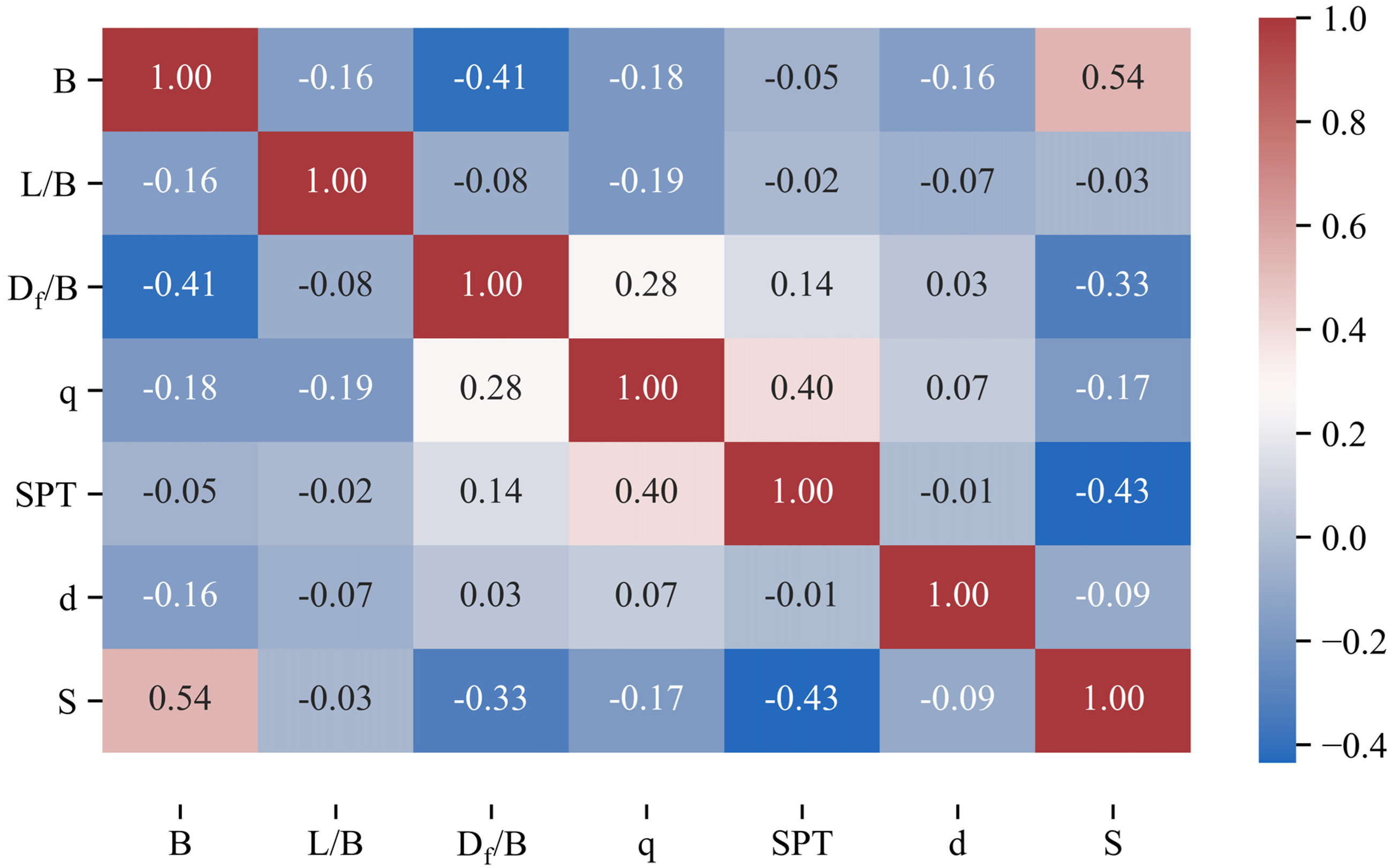
The values of the input variables are significantly correlated with the measured settlement as illustrated in Figure 2. The footing width correlated with the settlement has a positive linear relationship r = .54, p = .0000 (Figure 2(a)). In Figure 2(b), the scatters are quite random, the L/B values relative to the two-dimensional target are fairly uniform r = –0.03, and p = .6474. Figure 2(c) to (f) shows the negative linear relationship between the dependent variable settlement and the independent variables D_f/B (r = –.33, p = .0000), q (r = –.17, p = .0182), SPT (r = –.43, p = .0000), and d (r = –.09, p = .1992). In addition to the relationship between the independent and dependent variables, this section also considers each relationship between the variables illustrated in Figure 3. Figure 3 is the correlation matrix between the input variables and the measured settlement. The relationship between the variables from negative to positive is shown by the color range from blue to brick red. It explains that B and L/B have a correlation coefficient of −0.16 for their volatility. This shows that the correlation between B and L/B is negative. Similarly, the correlation between B and D_f/B, q, SPT, and d are all negative correlations. However, B and S have a correlation coefficient of 0.54, which indicates a positive linear relationship. L/B has a weak negative relationship with all variables. D_f/B is positively related to q, SPT, and d, but negatively related to S.

Figure 2.

Linear regression between each input variable and measured settlement.

Figure 3.

Pearson correlation of all variables.

Machine learning methods

Gradient boosting (GB)

Gradient Boosting (GB) enhances predictions through a technique called augmentation, which involves iteratively refining and correcting predictions that fall short in initial iterations.³⁷ The algorithm continues this process of correction until the desired accuracy is achieved. By focusing on reducing bias and variance, Gradient Boosting effectively transforms weak learners into strong ones. At its core, Gradient Boosting integrates multiple weak predictive models into a robust composite model. These weak models, which may only perform slightly better than random guessing, are combined to produce a stronger prediction model. The Boosting ensemble learning strategy can be mathematically expressed as follows:

F_{N} (x) = \sum_{n = 1}^{M} α_{n} f_{n} (x)

(1)

In this formula, F_N (x) represents the ensemble model formed by a linear combination of N basic models f_n(x) where α_n is the weight of the nth model.

The GB algorithm is grounded in the gradient descent method, applied to minimize a defined objective function:

E = \sum_{t = 1}^{T} L (y_{t}, F_{N} (x_{t}))

(2)

Here, T is the number of samples, N is the number of basic models, and L is the loss function. The training process sequentially optimizes each basic model f_n to minimize the objective function E.

According to gradient descent principles, the optimal model adjustment occurs in the direction of the negative gradient of the objective function:

f_{n} * (x) = \underset{f, α}{\arg min} \sum_{t = 1}^{T} L {(- \frac{\partial L}{\partial F_{n - 1} (x_{t})} - α \times f (x_{t}))}^{2}

(3)

This iterative process continues until all N basic models and their corresponding coefficients are trained. The final learning model, based on equation (1), leverages the Gradient Boosting algorithm's additive nature, where each subsequent model refines the accuracy achieved by previous models, effectively reducing the model bias. This approach contrasts with Bagging, as Gradient Boosting sequentially improves the accuracy of initially low-performing models, gradually enhancing the overall model's performance while balancing the risk of overfitting.

Random forest (RF)

In GB, trees are dependent on each other: They are built tree by tree, and the performance of the next tree is better than the previous tree (cost function optimization). Each tree will learn from the mistakes of the previous trees. In a Random Forest (RF), trees are built from random data samples and trained independently.³⁸ The overall score will then be based on the average score of the trees. The main difference between random forest and GB is the use of techniques. GB enhances the predictions with the help of a technique known as ‘boosting’. RF, on the other hand, enhances the predictions using a technique called ‘bagging’.

RF is developed based on decision trees. It can be used for both Classification and Regression problems in ML. As the name suggests, RF builds a forest at random, there are many decision trees in the forest and each decision tree in the forest has nothing to do with each other. A decision tree is a tree structure (which can be binary or non-binary). Each non-leaf node represents a test on a feature attribute, each branch represents the output of the feature attribute over a certain range of values, and each leaf node stores a category.

The reason to use different trees and not just one is that no single tree can always be the best. All trees are constructed with a random selection of attributes to split and a different number of splits is calculated by these attributes. Each node stores the attribute value (leaf) on which the split is performed. Randomness is included in the selection of features for each tree. Instead of looking for the most important feature while splitting a node, the algorithm chooses a random set of features to split a node for each tree generated. This allows for more modeling diversity, flexibility, less elemental clutter, and a less defined structure experience allowing for better out-of-sample performance and reduced risk of gearing exceed.

The specific implementation process of the random forest is as follows:

First, the bootstrap resampling method is used to randomly generate k $θ_{1}, θ_{2}, \dots θ_{k}$ training sets. Each training set can generate the corresponding decision tree ${T (x, θ_{1})}, {T (x, θ_{2})}, \dots {T (x, θ_{k})}$ and k is the number of trees in the random forest.

It is known that the size of the sample is M. During node splitting, N objects are randomly selected from the M-dimensional objects as the split feature set of this node. N is set only to the size of the sample, other improvement methods are not available. Usually, the value of N remains constant during the formation of the random forest.

For each tree that decides not to proceed with pruning, maximum growth can be set.

When there is new data X = x, the prediction of a single decision tree T (θ) can be obtained by averaging the observations of the leaf nodes l(x,θ). If an observation value X_i belongs to the leaf node l(x,θ) and not is 0, then the weight vector w is:

w_{i} (x, θ) = \frac{1 {X_{i} \in R_{i} (x, θ)}}{# {j : X_{j} (x, θ)}}

(4)

The sum of the weights w equals 1.

Given the independent variable X = x, the predicted value of a single decision tree is obtained by the weighted mean of the predicted value of the dependent variable Y_i (i = 1, 2, …n). The predicted value of a single decision tree is obtained according to equation (8):

\bar{μ} (x) = \sum_{i = 1}^{n} w_{i} (x, θ) Y_{i}

(5)

By averaging the decision tree weights

X = X_{i} (i \in {1, 2, \dots n})

and t = (1, 2, …k), the weight w_i(x) of each observation i ∈ (1, 2, …n) is obtained, see equation (9):

w_{i} (x, θ) = k^{- 1} \sum_{i = 1}^{k} w_{i} (x, θ) y

(6)

For all y, the prediction of random forest can be written as

\bar{μ}

Therefore, given the condition of X = x, the weighted sum of all dependent variable observations is the predicted mean. The weight changes with the change of the independent variable X = x, and the more similar the conditional distribution of Y under a given $X = X_{i} (i \in {1, 2, \dots n})$ is to the conditional distribution of Y under X = x, the greater the weight.

Support vector machine (SVM)

Support Vector Machine (SVM) is a two-class supervised learning model whose basic model is a linear model with the largest interval defined in the feature space.³⁹ The difference between SVM and the perceptron algorithm is that the perceptron only needs to find a hyperplane that can correctly divide the data, while the SVM needs to find the hyperplane with the largest interval to divide the data. So, there can be an infinite number of hyperplanes for the perceptron, but there is only one hyperplane for the SVM. In addition, SVM can handle nonlinear problems after introducing kernel functions.

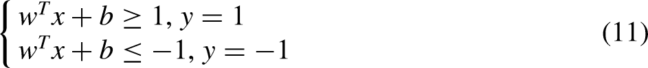
What SVM wants is to find the farthest distance from various sample points to the hyperplane, that is, to find the maximum interval hyperplane. Any hyperplane can be described by the following linear equation:

w^{T} x + b = 0

(7)

The formula for the distance from a two-dimensional space point (x, y) to the line Ax + By + C = 0 is:

\frac{| A x + B y + C |}{\sqrt{A^{2} + B^{2}}}

After expanding to n-dimensional space, the distance from point x = (x₁, x₂, …x_n) to line

w^{T} x + b = 0

\frac{| w^{T} x + b |}{‖ w ‖}

Where:

‖ w ‖ = \sqrt{w_{1}^{2} + \dots + w_{n}^{2}}

(8)

According to the definition of the support vector, the distance from the support vector to the hyperplane is d, and the distance from other points to the hyperplane is greater than d. So there is a formula like this:

{\begin{matrix} \frac{w^{T} x + b}{‖ w ‖} \geq d, y = 1 \\ \frac{w^{T} x + b}{‖ w ‖} \leq - d, y = - 1 \end{matrix}

(9)

A little transformation can get:

{\begin{matrix} \frac{w^{T} x + b}{‖ w ‖ d} \geq 1, y = 1 \\ \frac{w^{T} x + b}{‖ w ‖ d} \leq - 1, y = - 1 \end{matrix}

(10)

‖ w ‖ d

is a positive number, let it be 1 for the time being (for the convenience of derivation and optimization, and this has no effect on the optimization of the objective function), so:

{\begin{matrix} w^{T} x + b \geq 1, y = 1 \\ w^{T} x + b \leq - 1, y = - 1 \end{matrix}

(11)

Combining the two equations can be abbreviated as:

y (w^{T} x + b) \geq 1

(12)

So far, the upper and lower hyperplanes of the maximum interval hyperplane can be obtained. The distance from each support vector to the hyperplane can be written as:

d = \frac{| w^{T} x + b |}{‖ w ‖}

(13)

From the above

y (w^{T} x + b) > 1

, the

y (w^{T} x + b) = | w^{T} x + b |

can be obtained, so:

d = \frac{y (w^{T} x + b)}{‖ w ‖}

Maximize this distance:

max 2 \times \frac{y (w^{T} x + b)}{‖ w ‖}

(14)

Multiplying by 2 times here is also for later derivation and has no effect on the objective function. Just got the support vector

y (w^{T} x + b) = 1

, so:

max \frac{2}{‖ w ‖} min \frac{1}{2} ‖ w ‖

For the ease of calculation (remove the square of

‖ w ‖

min \frac{1}{2} ‖ w ‖^{2}

So the resulting optimization problem is:

min \frac{1}{2} ‖ w ‖^{2} : y_{i} (w^{T} x_{i} + b) \geq 1

(15)

K-Nearest neighbor (KNN)

The beauty behind a K-Nearest Neighbors (KNN) algorithm is that there's no need for training or learning. KNN does not provide a specific predictive model from the training data. Only when there is a prediction request for a certain object (label), the training data is used.

KNN is an algorithm where all computations are in the testing stage.⁴⁰ And, calculating the distance to each data point in the training set will take a lot of time, especially with databases with large dimensions and many data points. With a larger K, the complexity will also increase. In addition, storing all data in memory also affects the performance of KNN.

As mentioned above, the K-NN algorithm is to find the K closest to that instance in the training data set. Finding the distance between two points also has many formulas that can be used, depending on the case chosen accordingly.

Let the feature space X be n dimensions of the real number vector $R^{n}$ space, $x_{i}, x_{j} \in X$ , $x_{i} = (x_{i}^{1}, x_{i}^{2}, \dots, x_{i}^{n})^{T}$ , $x_{j} = (x_{j}^{1}, x_{j}^{2}, \dots, x_{j}^{n})^{T}$ , the distance L_p of $x_{i}, x_{j}$ is defined as:

L_{p} (x_{i}, x_{j}) = {(\sum_{l = 1}^{n} {| x_{i}^{l} - x_{j}^{l} |}^{p})}^{\frac{1}{p}}

(16)

Here p≥1, when p = 2, it is called the Euclidean distance, that is:

L_{2} (x_{i}, x_{j}) = {(\sum_{l = 1}^{n} {| x_{i}^{l} - x_{j}^{l} |}^{2})}^{\frac{1}{2}}

(17)

When p = 1, it is called the Manhattan distance, that is:

L_{1} (x_{i}, x_{j}) = \sum_{l = 1}^{n} | x_{i}^{l} - x_{j}^{l} |

(18)

When p = ∞, it is the maximum value of each coordinate distance, that is

L_{\infty} (x_{i}, x_{j}) = max_{l} | x_{i}^{l} - x_{j}^{l} |

(19)

Among them, when p = 2, it is the most common Euclidean distance. Generally, the Euclidean distance is used to measure the distance between two points in a high-dimensional space. In practical applications, the choice of the distance function should be based on the characteristics of the data and the needs of the analysis.

Particle swarm optimization (PSO)

Gradient-based methods require the problem space to be smooth and continuous, which is a major obstacle in solving real-world problems. Particle swarm optimization (PSO) is a heuristic that can operate on raw space and still produce a reasonable solution and is also more efficient and not greedy with storage requirements.⁴¹ This is a meta-heuristic optimization algorithm that can be applied to a large group of optimization problems. It does not make strict assumptions such as the distinct likelihood of the cost function. PSO is a powerful random optimization technique based on swarm movement and intelligence.⁴² PSO applies the concept of social interaction to problem-solving. It uses several agents (particles) that form a swarm that moves around in the search space to find the best solution.

The basic idea is to find the optimal solution through cooperation and information sharing among individuals in the group. Suppose there is only one beetle in the area and the whole flock of birds does not know where the food is. But they know how far away they are from the food, and they know where the bird is closest to the food. At the same time, each bird's distance from food is constantly changing as the position is constantly changing, so there must be a location closest to the food, which is also a reference for them. Therefore, there are two factors that affect the change in the bird's locomotion: The position of the bird closest to food, and the closest location ever to have food. In addition, there is one more factor that causes the position of the bird to change each time: inertia.

Each particle that tracks the coordinates of the bird in the solution space is associated with the best solution (fitness) that the particle has achieved so far. This value is called the personal best, Pbest.

Suppose a population consisting of Y individuals, each individual x repeats N times in search of food in Mx-dimensional space. Thus, at the ith loop, (i = 1, …, N) each individual x, (x = 1, …, Y) will have Mx positions, Mx velocities and is represented:

P_{i x} = {p_{i x}^{1}, \dots, p_{i x}^{M_{x}}}

(20)

V_{i x} = {v_{i x}^{1}, \dots, v_{i x}^{M_{x}}}

(21)

Where:

$p_{i x}^{k}$ is the position of individual x in the loop i at the dimension k, (k = 1, …, M _x )

$v_{i x}^{k}$ is the velocity of the individual x in the loop i at the dimension k, (k = 1, …, M _x )

Each individual based on its current velocity and the distance from Pbest _x to Gbest to change its position and adjust its velocity as follows:

v_{x}^{k + 1} = v_{x}^{k} + c_{1} z_{1} (P b e s t_{x} - s_{x}^{k}) + c_{2} z_{2} (G b e s t_{x} - s_{x}^{k})

(22)

The k-dimensional position update formula of particle x is:

s_{x}^{k + 1} = s_{x}^{k} + v_{x}^{k}

(23)

Where:

$x_{x}^{k}$ : current position of the individual x in the dimension k

$c_{1}, c_{2}$ : acceleration coefficient

$z_{1}, z_{2}$ : a random number between 0 and 1

$v_{x}^{k}$ : the velocity of individual x in the dimension k

K-Fold cross validation

Cross-validation is a statistical method used to estimate the performance of machine learning models. It is often used to compare and select the best model for a problem. This technique is easy to understand, easy to implement, and gives more reliable estimates than other methods. K-fold Cross-Validation (CV) is not the only way to prevent overfitting, but also to estimate how well models perform on brand-new data.^43,44 In K-fold cross-validation, the training data is divided into k parts or folds. The model is built on data from k-1 folds, each having the same dimensions, and tests the model on the remaining fold (validation set). It is possible to build variations of the model using different sets of parameters. Then, repeat this process k–1 times, each time excluding another time with model building (Figure 4).

Figure 4.

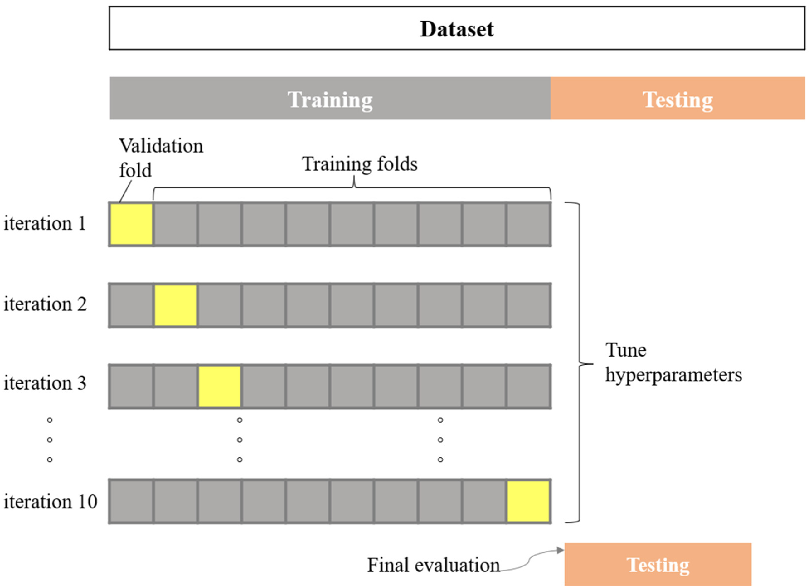
Conception of the ML approach for evaluating settlement of shallow foundation.

Partition data into distinct sets and use the test set to estimate how well the trained model will perform on the training data and how well it will perform on the unseen data. The training data is classified into two parts: the training set and the validation set. That is, divide the entire data set into three parts: training set, validation set, and test set. The training set is used to train the model and the validation set is used to evaluate the error of the model, then choose the one with the smallest error among the different models. The general steps are as follows: train different models through the training set, test the model with the valid set and choose the model with the smallest error to retrain the model with the training set's data + the validation set (i.e. initial training data) uses the test data to evaluate the selected model.

Shapley additive explanations

Shapley Additive Explanation (SHAP) is a technique in machine learning used for model interpretation.⁴⁵ It primarily applies linear modeling to locally estimate the impact of individual samples within complex machine learning models. SHAP helps reveal the contribution of each independent variable to the prediction of the target variable, offering clear visual explanations for why a particular data point has been predicted with a specific value. Unlike traditional algorithms, which rely on statistical rules and can be complex, SHAP provides easily interpretable visualizations that allow users to gauge the model's reliability for specific data points.

In scenarios where the model is nonlinear or input features are interdependent, SHAP values calculate a weighted average across all possible feature rankings. SHAP integrates these conditional expectations with classical Shapley values from game theory, assigning an attribution value to each feature as expressed by the following equation:

ϕ_{j} = \sum_{S \subseteq F ∖ {j}}^{\frac{| S |! (p - | S | - 1)!}{p!} (f (S \cup {j}) - f (S))}

(24)

Here, F represents the set of all input features, p is the total number of input features, S is a subset of features excluding j, and f(S) is the prediction based on the feature subset S.

The weights in the formula can be interpreted as follows: –

The denominator, p!, represents all possible combinations of the p features.

–

The numerator accounts for the number of combinations for a specific subset S, including all possible orderings of features within S, followed by the feature j, and then the remaining features.

In essence, the weight

\frac{| S |! (p - | S | - 1)!}{p!}

reflects the proportion of feature combinations associated with subset S, ensuring that the sum of all possible combinations equals 1.

Performance evaluation of the machine learning model

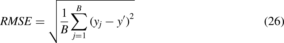
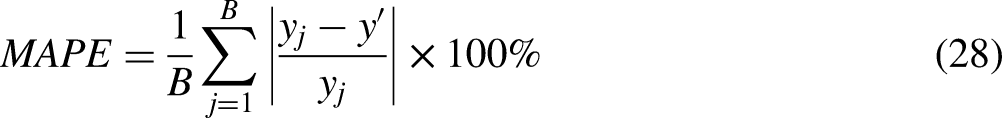
There is a saying that if want to do the job well, first sharpen the tools. Only when an accurate recording and measurement method is developed for the research problem can it be analyzed its nature and internal laws, researched in a targeted way, and solved. Evaluation indicators and the corresponding measurement methods are the foundation of modern science and key technology to promote the development of modern society, policy, and business. The evaluation indicators help to account for various risks and adverse factors, forming an overall assessment of the model. In this study, four measurements are used to evaluate the performance of the proposed model's coefficient of determination (R²), Root Mean Squared Error (RMSE), Mean Absolute Error (MAE), and Mean Absolute Percentage Error (MAPE). These four indicators are defined in turn as follows:

R^{2} = 1 - \frac{\sum {(y_{j} - y^{'})}^{2}}{\sum {(y_{j} - \bar{y})}^{2}}

(25)

R M S E = \sqrt{\frac{1}{B} \sum_{j = 1}^{B} {(y_{j} - y^{'})}^{2}}

(26)

M A E = \frac{1}{B} \sum_{j = 1}^{B} | y_{j} - y^{'} |

(27)

M A P E = \frac{1}{B} \sum_{j = 1}^{B} | \frac{y_{j} - y^{'}}{y_{j}} | \times 100 %

(28)

where B is the number of samples, y_j is the experimental value of compressive strength, and y’ is the predicted value.

Methodology flowchart

To effectively predict the settlement of shallow foundations, a structured methodology is applied, as outlined in the following steps. Each step is designed to enhance model accuracy and interpretability, from data preparation and hyperparameter tuning to model evaluation and feature impact analysis. This process aims to develop a robust predictive tool by combining traditional ML models with optimization techniques and advanced interpretative methods. The flowchart in Figure 5 provides an overview of the methodology used, summarized in the following steps:

Figure 5.

Conception of the ML approach for evaluating settlement of shallow foundation.

Step 1: The data is divided into two independent data sets, the training set and the test set. The training set is the dataset used to train the model, the training set includes the input vectors B, L, D_f, q, SPT, d and the corresponding settlement output vector. The test set does not participate in the training process, making the evaluation unbiased. According to the investigation of Nguyen et al.,⁴⁶ the training dataset and testing dataset can be split in a 70%/30% ratio for the best ratio of training/testing the ML model.

Step 2: To further improve the settlement of shallow foundation prediction performance, the PSO technique is used to tune the sets of hyperparameters. PSO combines with single models GB, RF, SVM, KNN to form hybrid models GB-PSO, RF-PSO, SVM-PSO, KNN-PSO. The sets of hyperparameters are evaluated by the error value of the RMSE model, the set of hyperparameters with the RMSE index is as low as possible.

Step 3: After obtaining the optimal parameters, these parameters are used to train the hybrid models GB-PSO, RF-PSO, SVM-PSO, and KNN-PSO. The performance of the models will be assessed by 10-fold CV, R², RMSE, MAE, and MAPE. Based on the results obtained on these criteria, four hybrid models were compared with four single models to select the models with the best performance. According to the recommendation of Kamali et al.,⁴⁷ all models undergo evaluation using 10-fold cross-validation to ensure robust validation, with RMSE (Root Mean Square Error) serving as the cost function to gauge prediction accuracy.

Step 4: Predict settlement of shallow foundation using models with optimal performance. The model with the best prediction results is used to analyze the effects of the variables. SHAP is used to assist in observing the complexity of the model's prediction results and the influence of the independent variables on the settlement of shallow foundation. Partial dependence plots (PDP) SHAP 1D help visualize trends in the impact of features on the settlement of shallow foundation.

The authors validate their methods by following a structured approach that ensures robust model performance and minimizes bias in the results. Here's how they ensure the validation of the data:

Data Splitting for Independent Testing: The dataset is split into training and testing sets in a 70%/30% ratio, based on findings from prior studies (e.g. Nguyen et al.⁴⁶), to ensure an unbiased evaluation. The training set is used solely to develop the models, while the test set, which remains unseen during training, is used to assess model performance, allowing for an independent measure of accuracy.

Cross-Validation (10-Fold CV): The models are further validated using 10-fold cross-validation, a technique that divides the training data into ten subsets. Each subset is used as a temporary testing set while the model is trained on the other nine. This process reduces overfitting and provides a more reliable measure of model performance on unseen data.

Hyperparameter Optimization with PSO: The Particle Swarm Optimization (PSO) algorithm is used to fine-tune model hyperparameters based on the root mean square error (RMSE) metric. Optimizing parameters reduces the risk of poor performance due to suboptimal model settings, improving generalization on the test set.

Performance Metrics: The authors assess each model using multiple performance metrics, including R², RMSE, Mean Absolute Error (MAE), and Mean Absolute Percentage Error (MAPE). This multi-metric evaluation ensures that the models are not only accurate but also reliable in various dimensions (e.g. error magnitude, explained variance), providing a comprehensive validation of model effectiveness.

Comparison with Baseline and Literature Models: By comparing the performance of hybrid models (e.g. GB-PSO) with single models (e.g. GB, RF, SVM, KNN) and reviewing results from previous literature, the authors benchmark their models against established standards. This helps verify that the proposed models either meet or exceed the performance of traditional methods.

Feature Contribution Analysis with SHAP including global values and partial dependence plots: To ensure the model is not only accurate but interpretable, SHAP (Shapley Additive Explanations) values and Partial Dependence Plots (PDPs) are used to examine the influence of each input feature. This validation step confirms that the model's predictions align with known domain knowledge about how certain features (e.g. SPT and footing width) affect foundation settlement.

Together, these steps help the authors validate their methods rigorously, ensuring that the models provide reliable predictions and insights into the foundation settlement data.

Table 3 outlines the hyperparameter tuning space employed for four machine learning models—Gradient Boosting (GB), Random Forest (RF), Support Vector Machine (SVM), and K-Nearest Neighbor (KNN)—to enhance the accuracy of foundation settlement predictions. Each model has distinct hyperparameters that influence its predictive performance, and selecting optimal values is crucial for achieving high accuracy.

Table 3.

Hyperparameters space of ML models in the tuned process.

Gradient boosting		Random forest		Support vector machine		K-nearest neighbor
Number of trees	1–40	Number of trees	1–40	Regularization parameter (C)	1–250	Number of neighbors	1–10
Learning rate	0.3–0.5	Number of trees	1–40	Regularization parameter (C)	1–250	Number of neighbors	1–10
Max features	1–4	Max features	1–4	Kernel coefficient Gamma (γ)	0.1–10	Leaf size	1–5
Max depth	1–5	Max depth	1–5			Leaf size	1–5
Min samples split	0.02–0.09	Min samples split	0.02–0.09			Power parameter p	1–5
Min samples leaf	0.02–0.09	Min samples leaf	0.02–0.09	Kernel type^a	1,2,3,4	Algorithm^b	1,2,3,4
Validation: 10-Fold CV Cost function: RMSE

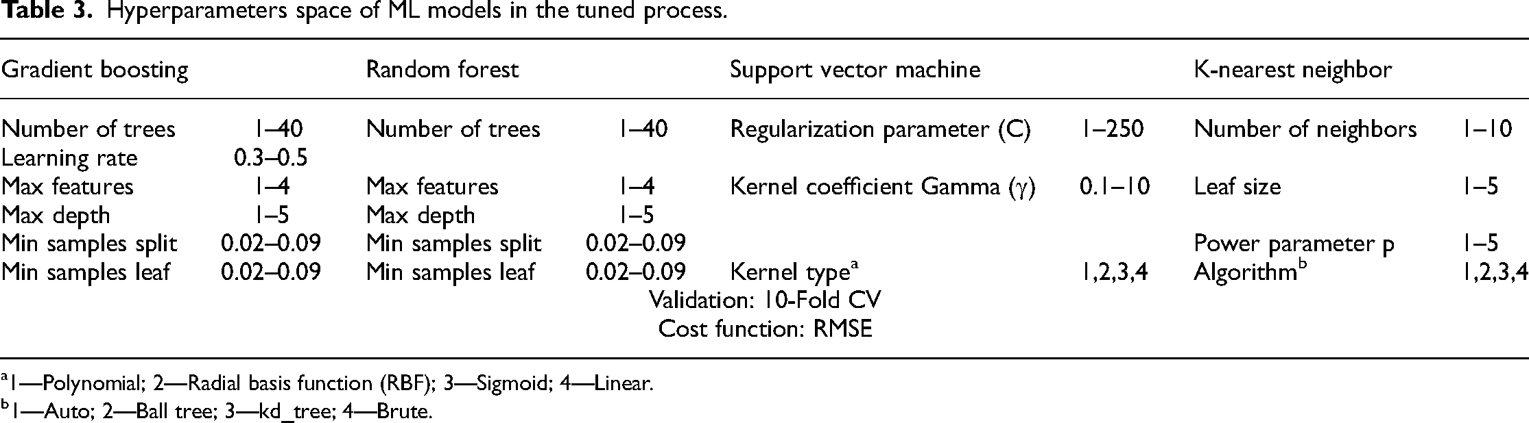
1—Polynomial; 2—Radial basis function (RBF); 3—Sigmoid; 4—Linear.

1—Auto; 2—Ball tree; 3—kd_tree; 4—Brute.

For Gradient Boosting (GB), key hyperparameters include the number of trees (ranging from 1 to 40), which defines the boosting stages; the learning rate (0.3–0.5), which adjusts the contribution of each tree; maximum features (1–4), controlling the subset of features for each split; maximum depth (1–5), which limits tree depth; minimum samples required to split a node (0.02–0.09); and minimum samples required to form a leaf node (0.02–0.09). These parameters are tuned to balance model complexity and prediction accuracy.

Random Forest (RF) shares similar hyperparameters with GB, including the number of trees (1–40), maximum features (1–4), maximum depth (1–5), and minimum samples for splits and leaves (both 0.02–0.09). These parameters collectively influence the robustness and generalization capability of the model.

For Support Vector Machine (SVM), the tuning space includes the regularization parameter (C, ranging from 1 to 250), which governs the trade-off between maximizing the margin and minimizing classification error; the kernel coefficient (γ, 0.1–10), which determines the influence of individual data points; and the kernel type, which can be Polynomial, Radial Basis Function (RBF), Sigmoid, or Linear. These choices impact SVM's flexibility and ability to model complex relationships.

Finally, K-Nearest Neighbor (KNN) tuning includes the number of neighbors (1–10), which sets the reference points for predictions; leaf size (1–5), affecting tree structures for search efficiency; power parameter (p, 1–5) that defines the distance metric; and the algorithm type, with options including Auto, Ball tree, kd_tree, and Brute for optimizing neighbor searches.

According to the recommendation of Kamali et al.,⁴⁷ all models undergo evaluation using 10-fold cross-validation to ensure robust validation, with RMSE (root mean square error) serving as the cost function to gauge prediction accuracy. This systematic exploration of hyperparameters enables the selection of optimal configurations, improving each model's predictive performance for shallow foundation settlement.

As reported by Blanke,⁴⁸ the values for parameters c1 and c2 of PSO model are assigned as 0.4, 0.7, and 0.7, respectively.

Results and discussion

Tunning hyperparameters of machine learning models

Figure 6 shows the change in the RMSE value for each population size value and number of iterations. The GB-PSO model has a decreasing RMSE value as the population size increases as seen in Figure 6(a). When the population size price reaches 100 the cost of the RMSE function is lowest. In Figure 6(b) it can be seen that as the flock size increases, the RF-PSO model becomes worse. The change in the number of individuals in the herd has almost no effect on the hyperparameter-adjusted results of the SVM-PSO model (Figure 6(c)). For the KNN-PSO model, the effect when the number of particles increases can be observed quite clearly when the number of iterations is small in Figure 6(d). The results show that the algorithms will refine the hyperparameter with a population size of 100.

Figure 6.

Effect of the population size on the cost function RMSE for tuning hyperparameters.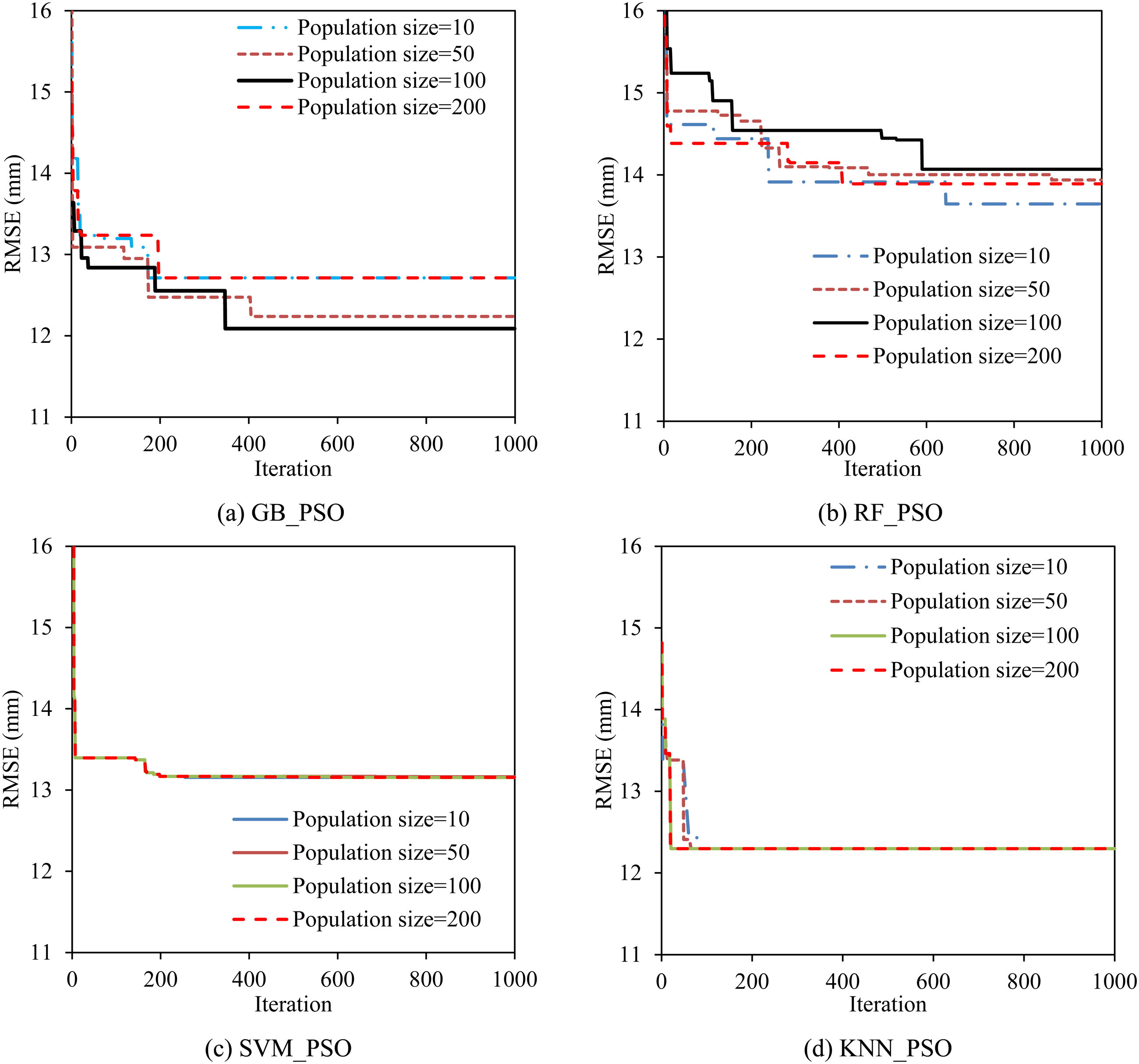

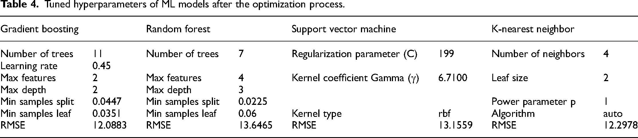
The GB model needs to adjust six parameters with the parameter Number of trees defining the number of trees as 11, the learning rate represents the learning rate = 0.45, and the max feature represents the maximum number of features to consider for separation. A node is 2, the hyperparameter max depth defines the complexity of the tree as 2, min samples split represents the minimum number of samples needed to split an inner node = 0.447, and min samples leaf is the number of samples The minimum required for a leaf node, was chosen to be 0.0351. Similarly, RF has five parameters to be adjusted: the number of trees seven, max feature four, max depth three, min samples split = 0.0225, and min samples leaf = 0.06. The SVM algorithm uses the RBF nonlinear multiplication function, with C = 199, gamma = 6.7100. KNN with a typical tree algorithm provides a method for allocating points in an automatically selected multi-dimensional space, number of neighbors four, leaf size two, power parameter p controlling the value of the Minkowski index method = 1. The hyperparameter parameters used for the RMSE models and cost function are summarized in Table 4. The results show that the GB model gives the best results with RMSE = 12.0883, followed by KNN with RMSE = 12.2978.

Table 4.

Tuned hyperparameters of ML models after the optimization process.

Gradient boosting		Random forest		Support vector machine		K-nearest neighbor
Number of trees	11	Number of trees	7	Regularization parameter (C)	199	Number of neighbors	4
Learning rate	0.45	Number of trees	7	Regularization parameter (C)	199	Number of neighbors	4
Max features	2	Max features	4	Kernel coefficient Gamma (γ)	6.7100	Leaf size	2
Max depth	2	Max depth	3			Leaf size	2
Min samples split	0.0447	Min samples split	0.0225			Power parameter p	1
Min samples leaf	0.0351	Min samples leaf	0.06	Kernel type	rbf	Algorithm	auto
RMSE	12.0883	RMSE	13.6465	RMSE	13.1559	RMSE	12.2978

Performance evaluation of machine learning models

After adjusting for hyperparameters, the models were re-evaluated using 10 fold CV and compared using the R², RMSE, MAE, and MAPE criteria. The GB-PSO, RF-PSO, SVM-PSO, and KNN-PSO hybrid models were compared with the original GB, RF, SVM, and KNN models to check optimized performance.

Figure 7 compares the performance obtained using the hybrid models GB-PSO, RF-PSO, SVM-PSO, and KNN-PSO. It can be seen that the GB-PSO model has a slightly higher R² value than the remaining models with R²-Mean = 0.8057 shown in Figure 7(a). The GB-PSO model also has the lowest value of RMSE-Mean of 12.8961, MAE-Mean of 8.6930, and MAPE-Mean of 0.7655 as illustrated in Figure 7(b) to (d), respectively.

Figure 7.

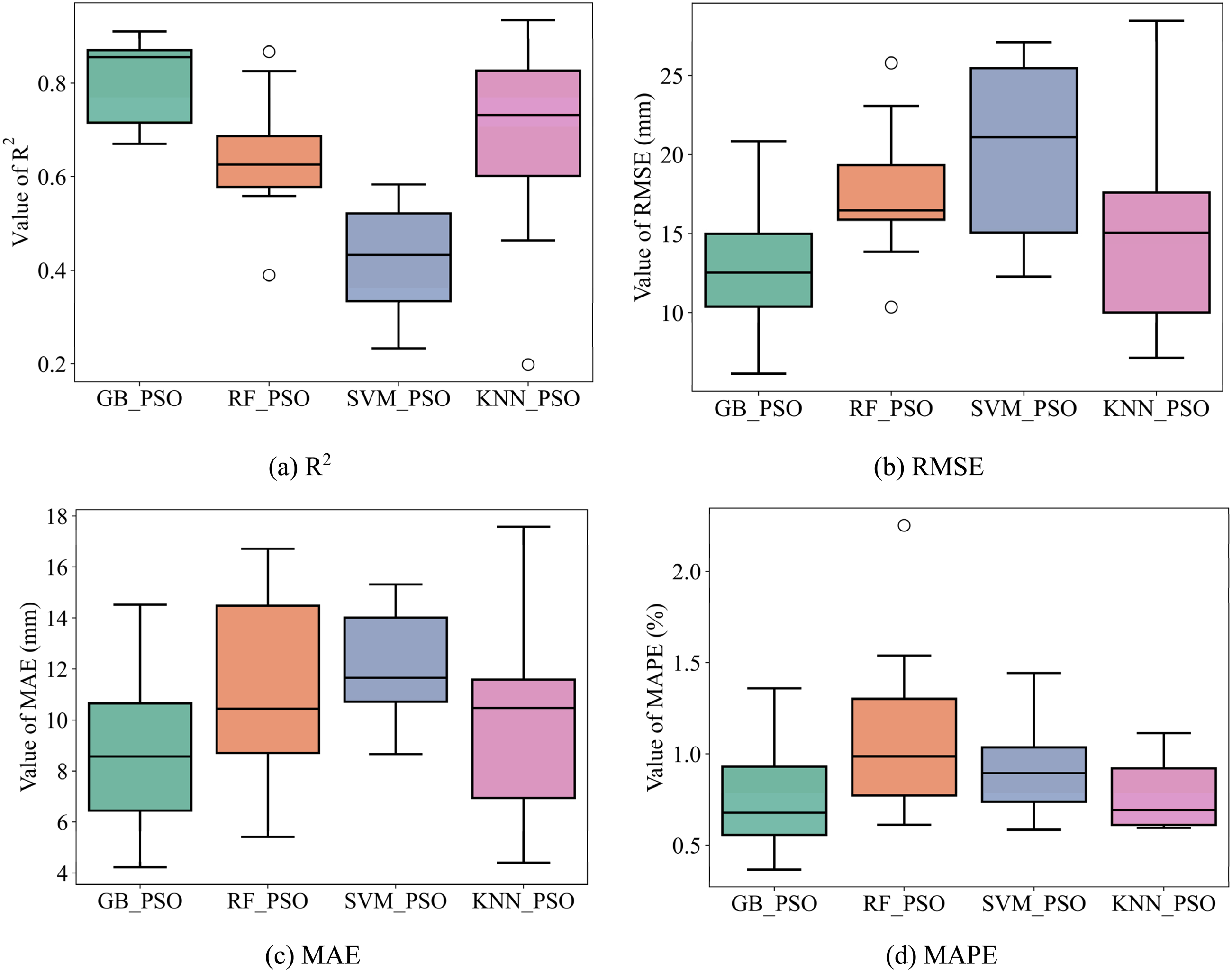
Performance comparison of 4 hybrid ML models with 10-Fold. (a) R², (b) RMSE, (c) MAE and (d) MAPE.

GB-PSO demonstrates the highest R² values, indicating superior predictive accuracy, while KNN-PSO follows closely. SVM-PSO has the lowest R², showing poorer model fit (cf. Figure 7(a)). GB-PSO achieves the lowest RMSE, reflecting minimal prediction error. RF-PSO and KNN-PSO display moderate error values, while SVM-PSO has the highest RMSE (cf. Figure 7(b)). Similarly, GB-PSO has the lowest MAE, with RF-PSO and KNN-PSO close behind, and SVM-PSO showing the largest absolute error values (cf. Figure 7(c)). GB-PSO and KNN-PSO achieve the lowest MAPE, indicating accurate percentage predictions. SVM-PSO again ranks the highest in error (cf. Figure 7(d)).

The results for the performance evaluation criteria of the hybrid models in terms of median, mean, and standard deviation are detailed in Table 5, the results are ranked in order from the model with the better performance. It can be seen that the GB-PSO and KNN-PSO models have better performance than the other mentioned hybrid models.

Table 5.

Median, mean and standard deviation value of 10-fold CV for 4 hybrid ML models.

	R²			RMSE			MAE			MAPE
	Median	Mean	SD	Median	Mean	SD	Median	Mean	SD	Median	Mean	SD
GB_PSO	0.8553	0.8057	0.0883	12.5397	12.8961	4.3497	8.5663	8.6930	2.8897	0.6776	0.7655	0.2949
KNN_PSO	0.7320	0.6856	0.2149	15.0580	15.3090	6.3963	10.4717	9.9566	3.7322	0.6928	0.7769	0.1916
RF_PSO	0.6261	0.6394	0.1293	16.4801	17.4840	4.2366	10.4438	11.2100	3.6516	0.9870	1.1291	0.4681
SVM-PSO	0.4329	0.4200	0.1188	21.1040	20.2313	5.7045	11.6540	11.9453	2.3190	0.8958	0.9435	0.2573

A comparison of the results of the addiction tests on the four initial models GB, RF, SVM, and KNN is shown in Figure 8. There are small differences between the R², RMSE, MAE, and MAPE values of the models. The SVM model has the lowest R² value of the four models, which can be clearly observed in Figure 8(a). The mean and median values of the R², RMSE, MAE, and MAPE criteria of the GB and RF models have very little difference in Figures 8(a) to (d).

Figure 8.

Performance comparison of 4 single ML models with 10-Fold. (a) R², (b) RMSE, (c) MAE and (d) MAPE.

GB and RF show similar, high R² values, indicating good predictive power, while KNN is slightly lower. SVM, however, has a significantly lower R² (cf. Figure 8(a)). GB and RF exhibit the lowest RMSE values, with KNN performing moderately well, and SVM showing the highest error (cf. Figure 8(b)). Consistent with RMSE, GB and RF models have the lowest MAE, followed by KNN and then SVM (cf. Figure 8(c)). Both GB and RF achieve low MAPE values, highlighting accurate prediction rates. KNN has a slightly higher MAPE, with SVM showing the highest (cf. Figure 8(d)).

Results from GB, RF, SVM, and KNN are compared and reported in Table 6, with better results ranked first. From Table 6, it can be seen that the two algorithms GB and RF have better performance, followed by the KNN model and finally the SVM model.

Table 6.

Median, mean and standard deviation value of 10-fold CV for 4 single ML models.

	R²			RMSE			MAE			MAPE
	Median	Mean	SD	Median	Mean	SD	Median	Mean	SD	Median	Mean	SD
GB	0.8664	0.8241	0.1219	11.1907	12.7622	4.1297	7.4169	7.1543	2.2973	0.5091	0.6113	0.3140
RF	0.7947	0.7695	0.1168	12.7241	13.5174	3.7352	7.3240	7.6337	2.5105	0.6053	0.6980	0.3636
KNN	0.6449	0.6309	0.2105	14.6791	16.2468	5.2454	9.8374	9.3812	2.4585	0.8906	0.9036	0.2523
SVM	−0.1249	−0.1268	0.0771	25.1808	26.2283	9.9350	13.7089	14.5200	5.5356	1.0247	1.0881	0.4270

According to the results, clearly the single GB, RF model performs better than the GB-PSO, RF-PSO hybrid model regardless of the R² or RMSE, MAE, or MAPE values. In contrast to GB-PSO, RF-PSO, hybrid models KNN-PSO and SVM-PSO have better performance, more efficient than single-model KNN and SVM. In summary, both single models and hybrid models have certain advantages. Four models with the best performance were selected to conduct the prediction: GB, RF, GB-PSO, and KNN-PSO.

Settlement prediction of four best machine learning models

Following the optimization of hyperparameters and model evaluation, four machine learning models GB-PSO, KNN-PSO, GB, and RF were applied to predict the settlement of shallow foundations. The performance of each model was assessed using four statistical metrics: coefficient of determination (R²), root mean square error (RMSE), mean absolute error (MAE), and mean absolute percentage error (MAPE). Both Figure 9 and Table 7 illustrate the differences in performance across these metrics for each model.

Figure 9.

Settlement prediction of shallow foundation using different ML models. (a) GB_PSO, (b) KNN_PSO, (c) GB and (d) RF.

Table 7.

Median, mean and standard deviation value of 10-Fold CV for 4 single ML models.

	R²			RMSE			MAE			MAPE
	Train	Test	All	Train	Test	All	Train	Test	All	Train	Test	All
GB	0.9866	0.9484	0.9742	3.0218	6.2528	4.2625	1.8196	4.2145	2.5419	0.1801	0.3967	0.2454
RF	0.9410	0.9308	0.9379	6.2839	7.3177	6.6127	3.5837	5.1446	4.0545	0.3059	0.4651	0.3539
GB_PSO	0.8819	0.8929	0.8849	9.5074	7.7125	9.0039	6.3658	5.7589	6.1828	0.6228	0.7188	0.6517
KNN_PSO	0.8191	0.8180	0.8190	11.5865	10.5773	11.2917	7.1284	6.8974	7.0587	0.7353	0.7298	0.7336

The scatter plot shows a significant deviation between experimental and predicted values, indicating that the GB-PSO model struggles with accuracy. Data points are widely scattered from the ideal Y = X line, suggesting that GB-PSO has difficulty generalizing accurately to both training and testing datasets (cf. Figure 9(a)). The KNN-PSO model exhibits similar behavior with a noticeable spread of points away from the best-fit line. This dispersion reflects higher error rates in the KNN-PSO model's predictions, demonstrating that this model is less reliable for precise settlement prediction (cf. Figure 9(b)). The GB model shows a much tighter alignment of data points along the Y = X line, suggesting high predictive accuracy. Most points are clustered close to the line, indicating that the GB model's predictions are quite close to actual settlement measurements. This model appears to have an exceptional fit, particularly in the training dataset (cf. Figure 9(c)). The RF model also shows relatively close clustering of data points around the ideal line, though not as precise as the GB model. There is some visible deviation, suggesting that while RF performs well, it is slightly less accurate than GB (cf. Figure 9(d)).

Table 7 provides numerical insights into each model's performance on both training and testing datasets, giving a comprehensive view of their predictive capabilities. With an R² value of 0.9866 in training and 0.9484 in testing, the GB model demonstrates the highest accuracy among the models. It has the lowest RMSE, MAE, and MAPE across datasets, which confirms it as the most accurate model for predicting settlement values. The results indicate that the GB model's predictions closely match the experimental data, with minimal error in both training and testing datasets. The RF model also performs well, with an R² of 0.9410 in training and 0.9308 in testing. Although not as accurate as the GB model, the RF model achieves relatively low RMSE, MAE, and MAPE values, making it a reliable alternative. However, it shows slightly higher error values compared to GB, especially in testing. The GB-PSO model shows moderate predictive performance, with an R2R^2R2 of 0.8819 in training and 0.8929 in testing. It has higher RMSE, MAE, and MAPE values, suggesting that while it captures some predictive accuracy, it is less effective than GB and RF. KNN-PSO demonstrates the lowest predictive accuracy among the four models. With an R² of 0.8191 in training and 0.8180 in testing, it has the highest RMSE, MAE, and MAPE values. This model's poor performance may be due to limitations in its learning capacity or sensitivity to dataset characteristics.

In summary, the GB model emerges as the best predictive model for shallow foundation settlement, with high accuracy and low error metrics in both training and testing datasets. The RF model follows as the second-best model, though with slightly higher error. The GB-PSO and KNN-PSO models are less effective, with KNN-PSO showing the lowest accuracy. Based on these results, the GB model is the most reliable choice for precise settlement prediction.

Table 8 provides a comparative analysis of the predictive performance of various machine learning (ML) models, as reported in previous studies, alongside the Gradient Boosting (GB) model applied in the current investigation. Each model's effectiveness is evaluated using three primary metrics: the coefficient of determination (R²), Root Mean Square Error (RMSE), and Mean Absolute Error (MAE) on the testing dataset. These metrics assess the accuracy, precision, and overall reliability of each model's prediction for foundation settlement. The GB model in this study achieves an R² of 0.948, indicating a very high degree of explained variance in settlement predictions. This is significantly higher than the results for Artificial Neural Network (ANN) and Genetic Programming (GP) models reported in prior studies by Shahin et al.²² 0.820 and Rezania and Javadi²³ 0.826, respectively. The GB model's superior R² suggests it captures more of the underlying complexity in the settlement data than earlier models. In terms of error metrics, the GB model exhibits the lowest RMSE 6.25 mm and MAE 4.21 mm values among all methods presented. These lower error values indicate that the GB model not only accurately predicts the settlement but also does so with higher precision and minimal deviations compared to other models, like the ANFIS-PSO hybrid used by Mohammed et al.,¹⁶ which, while optimized with Particle Swarm Optimization, shows higher errors RMSE = 9.02 mm, MAE = 6.50 mm. The dataset size for the GB model (189 samples) is comparable to those used by other studies, particularly Mohammed et al.¹⁶ (188 samples) and Shahin et al.²² (187 samples). Despite this, the GB model shows a clear advantage in both accuracy and precision, suggesting that Gradient Boosting, as applied in this study, effectively leverages similar data volumes to yield more reliable predictions. Interestingly, Erzin and Gul's model²⁴ reports a high R² of 0.990 despite having a small dataset (22 samples). However, with a smaller sample size, models can sometimes overfit, yielding high accuracy on specific data but risking reduced generalizability. By comparison, the GB model's strong performance on a larger dataset supports its robustness and suitability for broader applications.

Table 8.

Performance comparison between ML models of literature and ML models of this investigation.

Reference	Data	Method	Performance for testing dataset
Shahin et al.²²	187	ANN	R²= 0.820, RMSE = 11.04, MAE = 8.78
Rezania and Javadi²³	173	GP	R²= 0.826, RMSE = 11.07, MAE = 6.77
Erzin and Gul²⁴	22	ANN	R²= 0.990, RMSE = 1.79, MAE = 1.30
Mohammed et al.¹⁶	188	ANFIS-PSO	R²= 0.865, RMSE = 9.02, MAE = 6.50
Thiss investigation	189	GB	R²= 0.948, RMSE = 6.25, MAE = 4.21

Overall, the table illustrates the advantage of the Gradient Boosting model used in this study over earlier models in terms of both accuracy R² and error minimization RMSE, MAE. The findings suggest that GB, especially with optimal hyperparameter tuning, offers a promising, reliable approach for predicting foundation settlement, even outperforming complex hybrid models like ANFIS-PSO in practical engineering applications.

As a result, utilizing the Gradient Boosting (GB) model to predict the settlement of shallow foundations with high accuracy and low error is not only feasible but also potentially beneficial for developing numerical tools to assist in foundation settlement prediction. The GB model has demonstrated its robustness in handling the non-linear relationships between input variables and settlement outcomes. In practical applications, civil engineers can estimate the settlement of shallow foundations based on six input variables, utilizing an Excel file generated from the GB model's predictions (https://docs.google.com/spreadsheets/d/1jCoAbDTtDkNG0gN5slfpSaXdJTEZSTE6/edit?usp = drive_link&ouid = 106324620004270624859&rtpof = true&sd = true). This supplementary Excel tool can be used efficiently for rapid estimations, provided that the input variables remain within the prescribed value ranges for which the model was trained. Moreover, the model's predictions are highly dependent on the quality and range of the input data. If the variables fall outside the model's trained range, the predictions may become unreliable. Despite these challenges, the GB model remains a powerful tool for civil engineers, especially when used within its specified limitations. Future research could focus on overcoming these challenges by combining GB with other machine learning techniques or refining the hyperparameter tuning process to further enhance its practical application in foundation settlement predictions.

According to the authors’ research, previous studies on predictive models for shallow foundation settlement, including those by Shahin et al.,²² Rezania and Javadi,²³ Erzin and Gul,²⁴ and Mohammed et al.¹⁶ (listed in Table 1), used datasets with a maximum size of 188 samples. Expanding the dataset should be considered in future research to improve the predictive accuracy of the model.

Interpreting the contribution of each feature on the settlement of shallow foundation

Figure 10 presents the results of feature importance analysis for predicting the settlement of shallow foundations using two machine learning models: Gradient Boosting (GB) and Random Forest (RF). Panels (a) and (b) show SHAP (SHapley Additive exPlanations) values for the GB and RF models, respectively, illustrating the impact of each feature on model output. Here, SHAP values on the x-axis indicate the degree to which each feature influences settlement predictions, with positive values increasing predicted settlement and negative values decreasing it. Feature importance is visualized using color gradients from blue (low feature values) to pink (high feature values), indicating how each feature's value affects model predictions. For both models, the average SPT blow count feature has the strongest impact, as seen by the large SHAP values in Figures 10(a) and 10(b). As SPT values increase, their impact on settlement generally decreases. The width of the foundation (B) also shows significant influence in both models, whereas features like the depth of the water table (d) have a minimal effect.

Figure 10.

Feature importance analysis including Shapley additive explanations and permutation importance of sklearn.

Figure 10(c) and (d) displays the permutation importance of each feature for the GB and RF models, respectively, measured using the sklearn library. Permutation importance provides a model-agnostic measure of each feature's contribution by shuffling feature values and observing the impact on model performance. The permutation results confirm that SPT is the most influential feature, with B following as the second most important. In contrast, the feature “d” has a negligible effect on model predictions.

Table 9 summarizes the predictive performance of both models with two different feature sets: (i) using all six features, including the depth of water table (d), and (ii) using five features, excluding “d.” The table includes metrics such as R-squared (R²), Root Mean Squared Error (RMSE), Mean Absolute Error (MAE), and Mean Absolute Percentage Error (MAPE) for both the GB and RF models.

Table 9.

Performance comparison of two single ML models in two cases (i) with depth of water Table 6 input variables and (ii) without depth of water Table 5 input variables.

	GB				RF
	R²	RMSE	MAE	MAPE	R²	RMSE	MAE	MAPE
6 inputs	0.9484	6.2528	4.2145	0.3967	0.9308	7.3177	5.1446	0.4651
5 inputs	0.9473	6.3214	4.2697	0.4118	0.9229	7.7276	5.3827	0.4739
% Error	0.1201	1.0979	1.3099	3.8110	0.8558	5.6008	4.6282	1.8948

For the GB model, excluding “d” has a minimal effect on performance, with R² slightly decreasing from 0.9484 to 0.9473. However, for the RF model, removing “d” has a more noticeable impact, with R² dropping from 0.9308 to 0.9229. The percentage changes in RMSE, MAE, and MAPE values are also included, indicating that the RF model is more sensitive to the removal of “d” than the GB model.

In conclusion, both SHAP and permutation importance analyses indicate that SPT and B are the most influential factors in predicting settlement, while the depth of water table (d) has a negligible effect.

Figure 11 displays Partial Dependence Plots (PDPs) that illustrate the influence of several key variables on settlement predictions for shallow foundations. Each plot shows how variations in one input feature impact the settlement, as indicated by the SHAP (SHapley Additive exPlanations) values on the vertical axis. Red data points represent individual samples, helping visualize trends between each feature and its impact on settlement.

Figure 11.

Influence of each feature on the settlement of shallow foundation using SHAP partial dependence plot.

Figure 11(a) shows the relationship between the average SPT blow count and settlement. There is a clear negative correlation, as indicated by a steep decline in SHAP values as SPT values increase. This trend suggests that higher SPT values, which reflect denser soil, contribute to reduced settlement. This inverse relationship is prominent, with SHAP values becoming negative as SPT reaches higher levels.

Figure 11(b) examines the effect of footing width B on settlement. The SHAP values increase significantly with increasing B, indicating a strong positive influence. This suggests that larger footing widths lead to increased settlement, as shown by the upward trend in SHAP values with larger B values.

Figure 11(c) illustrates the effect of the footing embedment ratio D_f/B on settlement. Here, SHAP values decrease sharply when D_f/B is between 0 and 1, indicating a substantial initial impact on settlement. Beyond this range, SHAP values stabilize, showing minimal fluctuations. This pattern implies that the embedment ratio's influence on settlement is most pronounced at lower values and becomes negligible as D_f/B increases.

Figure 11(d) shows the relationship between footing net applied pressure q and settlement. The SHAP values increase almost linearly as q rises from 0 to around 200 kPa, indicating that increasing q generally increases settlement. After 200 kPa, the rate of change in SHAP values slows, suggesting that the influence of q on settlement diminishes at higher pressures.

Figure 11(e) and (f) depicts the effects of the footing geometry ratio L/B and the depth of water table d, respectively. In both plots, SHAP values are concentrated near zero, with most data points tightly clustered, indicating that these features have relatively minor and negligible impacts on settlement. Any influence is mostly limited to a few outliers, suggesting that L/B and d do not significantly contribute to settlement predictions.

In summary, Figures 11(a) to (f) reveal that SPT and B are the most influential factors, with SPT having a negative effect and B a positive effect on settlement. The embedment ratio D_f/B and applied pressure q also affect settlement but to a lesser extent. The variables L/B and d show minimal impact, with SHAP values close to zero for most samples, indicating their limited role in influencing settlement predictions.

These observations align with experimental findings from Shahin et al.²² and Rezania and Javadi,²³ which highlighted the significant role of SPT in predicting settlement. The importance of SPT in influencing settlement has also been supported by earlier studies, including those by Terzaghi and Peck (1967),⁴⁹ Fletcher,⁵⁰ and Shahin (2005).⁵¹ In line with previous research and design charts,^36,52,53 the analyses indicate that SPT and BBB have opposing influences on settlement, with SPT reducing settlement and BBB increasing it. While D_f/B and q exhibit moderate influence on settlement, particularly at lower values, L/B and d demonstrate minimal impact on the settlement predictions of shallow foundations, except for a few outliers.

Conclusions and perspectives

This study introduces a novel approach to accurately predict settlement in shallow foundations by leveraging four machine learning (ML) models: Gradient Boosting (GB), Random Forest (RF), Support Vector Machine (SVM), and K-Nearest Neighbors (KNN). Each model is optimized through Particle Swarm Optimization (PSO) and rigorously evaluated using 10-fold cross-validation with RMSE as the cost function. Our findings highlight the capability of these models to approximate settlement behavior, with the GB model achieving the highest predictive accuracy (R² = 0.9484) on the testing dataset. Despite applying hybrid modeling techniques, the original models outperformed these combinations, suggesting that simpler models may yield better performance when data is limited or noisy.

A significant contribution of this study lies in its in-depth analysis of feature importance in settlement prediction. Through SHAP global values and SHAP Partial Dependence Plots, we observe that the average SPT blow count and footing width B are the most influential variables, with opposing effects on settlement; SPT has a negative impact, while B has a positive one. The footing embedment ratio D_f/B and applied pressure q also affect settlement but exhibit non-linear influences, changing significantly at low values and stabilizing thereafter. The remaining factors, footing geometry L/B and water table depth d, have minimal impact, as shown by their near-zero SHAP values.

This study is pioneering in its development of an Excel-based tool derived from the Gradient Boosting model, enabling civil engineers to estimate foundation settlement using six key input variables. This tool, calibrated within specific data ranges, provides a practical and user-friendly interface for field applications, marking a novel contribution toward accessible computational design tools in geotechnical engineering.

Moreover, the findings underscore an important insight: ML models with default hyperparameters can sometimes outperform those with tuned parameters in cases of limited or noisy data. Hyperparameter tuning, while typically beneficial, may overfit when the dataset is small or imbalanced. This result emphasizes the need for high-quality, well-distributed datasets to improve model reliability and suggests that, in such cases, conservative default settings might be preferable for generalization.

In summary, this investigation not only provides a robust predictive framework for shallow foundation settlement but also highlights practical considerations in ML modeling, such as the risk of overfitting during hyperparameter tuning. Future work will focus on expanding the dataset and addressing data quality issues to further enhance model performance and generalization, paving the way for even more accurate and reliable predictions in foundation design.

Footnotes

Nomenclature

Authors’ contribution

Thi Thanh Huong Ngo contributed to conceptualization, methodology, visualization, writing–original draft, writing–review and editing, and validation. Van Quan Trans contributed to data curation, conceptualization, methodology, software, visualization, writing–original draft, writing–review and editing, and validation.

Availability of data and material

Data will be made available on request.

Declaration of conflicting interests

The authors declared no potential conflicts of interest with respect to the research, authorship, and/or publication of this article.

Ethical approval

This article does not contain any studies with human participants or animals performed by any of the authors.

Funding

The authors received no financial support for the research, authorship, and/or publication of this article.

Informed consent

This research does not involve any human participants or animals.

ORCID iD

Van Quan Tran

References

Dappolonia

Brissette

. Settlement of spread footings on sand. J Soil Mech Found Div 1968; 94. https://trid.trb.org/view/126934 (accessed 30 May 2022).

Alpan

. Estimating the settlements of foundations on sands. Civ Eng Public Works Rev UK 1964; 59: 700. https://trid.trb.org/view/139697 (accessed 30 May 2022).

Meyerhof

. Shallow foundations. J Soil Mech Found Div May 1966; 92: 4824. https://trid.trb.org/view/38525 (accessed 30 May 2022).

Berardi

Lancellotta

. Stiffness of granular soils from field performance. Geotechnique 1991; 41: 149–157. https://trid.trb.org/view/364773 (accessed 30 May 2022).

Zhu

Karakus

, et al. Investigating toppling failure mechanism of anti-dip layered slope due to excavation by physical modelling. Rock Mech Rock Eng 2020; 53: 5029–5050.

Zhang

, et al. State-of-the-art review of soft computing applications in underground excavations. Geosci Front 2020; 11: 1095–1106.

Liu

Ren

, et al. Multiscale laboratory study and numerical analysis of water-weakening effect on shale,” adv. Mater Sci Eng 2020; 2020: e5263431.

Elsharawy

. The effect of 3D interference of shallow foundation on settlement and its impacts on building structures. Civ Eng Archit 2024; 12: 2074–2090.

Bowles

. Foundation analysis and design. 5th ed. New York: McGraw-Hill, 1996.

10.

Boiko

Alhassan

. Effect of vertical cross-sectional shape of foundation on settlement and bearing capacity of soils. Procedia Eng 2013; 57: 207–212.

11.

Rahardjo

Nio

Leong

, et al. Effects of groundwater table position and soil properties on stability of slope during rainfall. J Geotech Geoenvironmental Eng 2010; 136: 1555–1564.

12.

Zhang

Hong

, et al. Comprehensive review of machine learning in geotechnical reliability analysis: algorithms, applications and further challenges. Appl Soft Comput 2023; 136: 110066.

13.

Wang

Xia

Gong

, et al. Multi objective optimization of recycled aggregate concrete based on explainable machine learning. J Clean Prod 2024; 445: 141045.

14.

Wang

, et al. Prediction and optimization model of sustainable concrete properties using machine learning, deep learning and swarm intelligence: a review. J Build Eng 2023; 80: 108065.

15.

Hasanzadehshooiili

Mahinroosta

Lakirouhani

, et al. Using artificial neural network (ANN) in prediction of collapse settlements of sandy gravels. Arab J Geosci 2014; 7: 2303–2314.

16.

Mohammed

Sharafati

Al-Ansari

, et al. Shallow foundation settlement quantification: application of hybridized adaptive neuro-fuzzy inference system model. Adv Civ Eng 2020; 2020: e7381617.

17.

Samui

. Support vector machine applied to settlement of shallow foundations on cohesionless soils. Comput Geotech 2008; 35: 419–427.

18.

Zhai

. Machine-learning-based road soft soil foundation treatment and settlement prediction method. Sci Program 2022; 2022: –7.

19.

Soleimani

Jiao

Rajaei

, et al. A new approach for prediction of collapse settlement of sandy gravel soils. Eng Comput 2018; 34: 15–24.

20.

Shahnazari

Shahin

Tutunchian

. Evolutionary-based approaches for settlement prediction of shallow foundations on cohesionless soils. Int J Civ Eng 2014; 12: 55–64.

21.

Song

Liu

Jiang

, et al. Research on the settlement prediction model of foundation pit based on the improved PSO-SVM model. Sci Program 2022; 2022: –9.

22.

Shahin

Jaksa

Maier

. Artificial neural network-based settlement prediction formula for shallow foundations on granular soils. Aust Geomech 2002; 37: 45–52.

23.

Javadi

Rezania

Nezhad

. Evaluation of liquefaction induced lateral displacements using genetic programming. Comput Geotech 2006; 33: 222–233.

24.

Erzin

Gul

. The use of neural networks for the prediction of the settlement of one-way footings on cohesionless soils based on standard penetration test. Neural Comput Appl 2014; 24: 891–900.

25.

Raja

MNA

Shukla

. Predicting the settlement of geosynthetic-reinforced soil foundations using evolutionary artificial intelligence technique. Geotext Geomembr 2021; 49: 1280–1293.

26.

Meyerhof

. Shallow foundations. J Soil Mech Found Div Mar. 1965; 91: 21–31.

27.

Terzaghi

Peck

Mesri

. Soil Mechanics in Engineering Practice. 3rd edition. New York: Wiley-Interscience, 1996.

28.

Parry

. A direct method of estimating settlements in sand from SPT values. Presented at the (paper to) Symposium on Interaction of Structure and Foundations, 1972, Midlands Soil Mechanics and Foundation Engineering Society, United Kingdom, 1985. https://trid.trb.org/view/1194069 (accessed 30 May 2022).

29.

Peck

Hanson

Thornburn

. Foundation Engineering. [By] R.B. Peck … Walter E. Hanson … Thomas H. Thornburn. Pp. xix. 410. John Wiley & Sons: New York; Chapman & Hall: London, 1953.

30.

Burland

Burbidge

Wilson

. Settlement of foundations on sand and gravel. Proc Inst Civ Eng 1985; 78: 1325–1381.

31.

Friedman

. Stochastic gradient boosting. 2002. doi: 10.1016/S0167-9473(01)00065-2.

32.

Breiman

. Random forests. Mach Learn 2001; 45: 5–32.

33.

Cortes

Vapnik

. Support-vector networks. Mach Learn Sep. 1995; 20: 273–297.

34.

Altman

. An Introduction to kernel and nearest-neighbor nonparametric regression. Am Stat 1992; 46: 175–185.

35.

Kennedy

Eberhart

. Particle swarm optimization. In: Presented at the proceedings of ICNN’95-international conference on neural networks. Nagoya, Japan: IEEE, 1995, pp.1942–1948.

36.

Shahin

Maier

Jaksa

. Predicting settlement of shallow foundations using neural networks. J Geotech Geoenvironmental Eng 2002; 128: 785–793.

37.

Friedman

. Greedy function approximation: a gradient boosting machine. Ann Stat 2001; 29: 1189–1232.

38.

Breiman . Random forests. Mach Learn 2001; 45: 5–32.

39.

Cortes

Vapnik

. Support-vector networks. Mach Learn 1995; 20: 273–297.

40.

Dudani

. The distance-weighted k-nearest-neighbor rule. IEEE Trans Syst Man Cybern Apr. 1976; SMC-6: 325–327.

41.

Eberhart

Kennedy

. A new optimizer using particle swarm theory. MHS’95 Proceedings of the Sixth International Symposium on Micro Machine and Human Science 1995: 39–43. doi: 10.1109/MHS.1995.494215

42.

Wang

, et al. A correlation-based binary particle swarm optimization method for feature selection in human activity recognition. Int J Distrib Sens Netw 2018; 14: 1550147718772785.

43.

François

Rossi

Wertz

, et al. Resampling methods for parameter-free and robust feature selection with mutual information. Neurocomputing 2007; 70: 1276–1288.

44.

Diamantidis

Karlis

Giakoumakis

. Unsupervised stratification of cross-validation for accuracy estimation. Artif Intell 2000; 116: 1–16.

45.

Lundberg

Lee

S-I

. A unified approach to interpreting model predictions. In: Proceedings of the 31st international conference on neural information processing systems, in NIPS’17. Red Hook, NY, USA: Curran Associates Inc., Tháng Mười Hai, 2017, pp.4768–4777.

46.

Nguyen

, et al. Influence of data splitting on performance of machine learning models in prediction of shear strength of soil. Math Probl Eng 2021; 2021: 1–15.

47.

Zanganeh Kamali

, et al. Permeability prediction of heterogeneous carbonate gas condensate reservoirs applying group method of data handling. Mar Pet Geol 2022; 139: 105597.

48.

Blanke

. Hyperactive: An optimization and data collection toolbox for convenient and fast prototyping of computationally expensive models. 2019. https://github.com/SimonBlanke .

49.

Terzaghi

Peck

Mesri

. Soil Mechanics in Engineering Practice. New York, USA: John Wiley & Sons, 1996.

50.

Fletcher

GFA

. Standard penetration test’ its uses and abuses. J Soil Mech Found Div 1965; 91: 67–75. https://trid.trb.org/view/120133 (accessed 30 May 2022).

51.

Shahin

Jaksa

Maier

. Neural network based stochastic design charts for settlement prediction. Can Geotech J 2005; 42: 110–120.

52.

Lutenegger

DeGroot

Windoloski

. “Compendium Of Case Histories Of Settlement Of Shallow Foundations On Granular Soil Deposits,” Art. no. UMTC-94-4A, Feb. 1995, https://trid.trb.org/view/703228 (accessed 30 May 2022).

53.

Leonards

Frost

. Settlement of shallow foundations on granular soils. J Geotech Eng 1988; 114: 791–809.

Predicting and evaluating settlement of shallow foundation using machine learning approach

Abstract

Keywords

Highlights

Introduction

Literature review

Database description and analysis

Machine learning methods

Gradient boosting (GB)

Random forest (RF)

Support vector machine (SVM)

K-Nearest neighbor (KNN)

Particle swarm optimization (PSO)

K-Fold cross validation

Shapley additive explanations

Performance evaluation of the machine learning model

Methodology flowchart

Results and discussion

Tunning hyperparameters of machine learning models

Performance evaluation of machine learning models

Settlement prediction of four best machine learning models

Interpreting the contribution of each feature on the settlement of shallow foundation

Conclusions and perspectives

Footnotes

Nomenclature

Authors’ contribution

Availability of data and material

Declaration of conflicting interests

Ethical approval

Funding

Informed consent

ORCID iD

References