Sage Journals: Discover world-class research

Abstract

In contemporary society, commercial buildings, as a crucial component of urban development, face increasingly prominent energy consumption issues, posing significant challenges to the environment and sustainable development. Traditional energy management methods rely on empirical models and rule-based approaches, which suffer from low prediction accuracy and limited applicability. To address these issues, this study proposes a commercial building energy consumption prediction and energy-saving strategy model based on hybrid deep learning and optimization algorithms. This model integrates convolutional neural networks (CNN), gated recurrent units (GRU), and the clonal selection algorithm (CSA), aiming to enhance the accuracy and efficiency of energy consumption predictions. Experimental results demonstrate that the CNN-GRU-CSA Network (CGC-Net) model achieves mean absolute errors (MAE) of 17.12, 16.73, 16.62, and 15.94 on the Building Data Genome Project (BDGP), Commercial Building Energy Consumption Survey (CBECS), Nonresidential Building Energy Performance Benchmark (NEPB), and Building Energy Efficiency Benchmark (BEBDEE) datasets, respectively, significantly outperforming traditional methods and other models. Additionally, the model exhibits faster inference and training times. These results validate the stability and superiority of the CGC-Net model, providing an innovative solution and essential technical support for commercial building energy management.

Keywords

Commercial buildings energy consumption prediction energy saving strategies deep learning models building energy management sustainability optimization

Introduction

As an important part of urban development, commercial buildings play a key role in promoting economic growth and social progress. However, with the acceleration of urbanization and economic development, the problem of energy consumption of commercial buildings is becoming increasingly prominent, which poses a great challenge to the environment and sustainable development.¹ Effective management of energy consumption of commercial buildings and improving energy efficiency have become important problems to be solved urgently.²

Traditional energy management methods mainly rely on empirical models and rule-making, and have problems such as low prediction accuracy and limited applicability.³ In recent years, the development of deep learning technology has provided a new perspective for building energy consumption prediction. Deep learning models show significant advantages in the field of building energy consumption prediction with their powerful data processing ability and adaptive learning ability.^4,5 However, the existing models are often limited by the neglect of the integration of spatial and temporal series information, resulting in insufficient prediction accuracy and generalization abilities.^6,7

To overcome these limitations, this paper proposes a novel prediction model. On the basis of the existing research, this paper first reviews the deep learning-based building energy consumption prediction methods, including convolutional neural network (CNN), gating cycle unit (GRU), etc. and discusses their potential and limitations in capturing the spatial and temporal characteristics of building energy consumption. Furthermore, this paper clarifies the research gap, namely the existing model in the processing of large-scale, high dimensional building energy consumption data, and to put forward the CNN-GRU-CSA Network (CGC-Net) model, the model comprehensive use of CNN spatial feature extraction ability, GRU time series analysis advantage and clonal selection algorithm (CSA) optimization strategy, in order to achieve more accurate energy consumption prediction.

The contribution points of this paper are as follows:

The design of the CGC-Net model, employing a hybrid deep learning framework that combines CNN, GRU, and CSA, effectively leveraging spatial and temporal information to achieve accurate energy consumption prediction for commercial buildings.

The proposal of a model optimization method based on the CSA, which effectively adjusts the parameters and structure of CNN and GRU models, enhancing the model's performance and generalization capabilities, and providing significant application value.

An in-depth exploration of the application of deep learning models in energy consumption prediction and energy-saving strategy formulation for commercial buildings, addressing practical needs in the field of commercial building energy management, and providing important references and support for improving energy utilization efficiency and achieving sustainable development goals.

The structure of this paper is as follows: Related work section introduces related work, including the current state of commercial building energy management and the application of deep learning in this field; Methodology section presents the research methods and model design used in this study, including the construction and optimization of the CGC-Net model; Experiment section validates the proposed model through experiments and analyzes the results; the final section summarizes the paper and discusses future research directions.

Related work

In the field of building energy consumption prediction, significant progress has been made in the application of deep learning models. This section will be divided into four parts to introduce the research progress and results of different deep learning models in commercial building energy consumption prediction.

Predicting building energy consumption using LSTM

Long-and short-term memory network (LSTM) is a special RNN, whose core principle is to effectively capture the long-term dependencies in time series data through the gating mechanism.⁸ Hochreiter and Schmidhuber proposed the LSTM model in 1997, aiming to solve the problem of gradient disappearance and gradient explosion of traditional RNN models when handling long sequence data, and thus to be more suitable for processing time series data. In the field of energy consumption prediction of commercial buildings, the LSTM model is widely used in the modeling and prediction of building energy consumption data, and its advantages in time series data modeling make it an important tool for processing the energy consumption data of commercial buildings.⁹

However, although the LSTM model has made significant achievements in forecasting energy consumption in commercial buildings, it has limited prediction power when dealing with extreme situations (e.g. abnormal weather conditions or emergencies).^10,11 In addition, LSTM models also face challenges in modeling seasonal and cyclical changes in building energy consumption data, requiring further optimization to improve the generalization ability and applicability of the models.¹² To address these problems, researchers are exploring ways to optimize the structure and parameters of LSTM models, and combining other deep learning models and traditional methods to explore multi-model integration strategies to further improve the accuracy and stability of building energy consumption prediction.¹³

Predicting building energy consumption using Transformer

The Transformer model is a deep learning model based on the Self-Attention Mechanism. It was proposed by Vaswani et al. in 2017. It aims to solve the long-distance dependency problem in sequence-to-sequence tasks, such as machine translation. Its core principle is to use the Self-Attention Mechanism to achieve information interaction and correlation learning at different positions in the sequence, thereby better capturing long-distance dependencies in sequence data.¹⁴

Transformer models are widely applied in the processing and prediction of building energy consumption data. Compared to traditional recurrent neural networks, Transformer models exhibit superior parallelism and efficiency when handling long sequence data.¹⁵ This capability enables them to more effectively capture temporal features in building energy consumption data, thereby enhancing the stability of energy consumption forecasts.¹⁶ The Self-Attention Mechanism allows Transformer models to flexibly capture both local and global correlations in the data, unrestricted by sequence length, making them suitable for energy consumption prediction tasks across various time scales.² Furthermore, Transformer models demonstrate strong generalization capabilities, capable of handling diverse types and scales of building energy consumption data, providing a more reliable and effective solution for commercial building energy consumption management.¹⁷

Although the Transformer model has many advantages in commercial building energy consumption prediction, it still faces some challenges. For example, the computing and storage costs of models are high, and there are certain limitations in processing large-scale building energy consumption data. In addition, when processing time series data, the model may be affected by factors such as data sampling frequency and data noise, resulting in reduced prediction performance.¹⁸

The current research trend mainly lies in optimizing the structure and parameters of the Transformer model to improve its performance and efficiency in commercial building energy consumption prediction. At the same time, combined with other deep learning models and traditional methods, multi-model integration strategies are explored to further improve the accuracy and robustness of building energy consumption prediction.¹⁹ In addition, in view of the computing and storage cost issues of the Transformer model, it is also a popular direction to explore methods of model compression and acceleration to achieve efficient prediction and application on large-scale commercial building energy consumption data.²⁰ For instance, a recent study demonstrated the integration of wavelet transform with the Transformer architecture for household energy consumption prediction, significantly improving the accuracy and efficiency of the forecasts.²¹

Predicting building energy consumption using generative adversarial network (GAN)

GAN is an adversarial learning framework composed of a generator and a discriminator, which was proposed by Goodfellow et al. in 2014. The core principle is to generate realistic samples through the generator, and evaluate the authenticity of the generated samples through the discriminator.²² The two networks compete with each other and are continuously optimized. Finally, the generator can generate samples similar to real data.

GAN models are mainly used in the generation, enhancement, and repair of building energy consumption data. By training the generator model to generate realistic building energy consumption data, GAN can expand the original data set and improve the generalization ability and robustness of the building energy consumption prediction model.²³ At the same time, the GAN model can also be used for data repair and denoising, further improving the accuracy and reliability of building energy consumption prediction. In commercial building energy consumption prediction, the GAN model can generate realistic building energy consumption data, thus enriching the data set and improving the generalization ability of the prediction model. In addition, the GAN model can also solve the problem of data imbalance by generating samples, improving the adaptability of the prediction model to different energy consumption levels.²⁴

Although GAN models offer numerous advantages in predicting commercial building energy consumption, they still face certain challenges. The quality of the generated samples can be significantly influenced by the training dataset. If the original dataset lacks high quality, the generated samples may exhibit bias.²⁵ In addition, the training process of the GAN model is relatively complex and requires careful parameter adjustment and selection of an appropriate loss function to obtain stable training effects.

The current main research direction is to improve the generation quality and stability of GAN models, which can improve the application effect in commercial building energy consumption prediction.²⁶ At the same time, researchers are also trying to combine other deep learning models and traditional methods to explore multi-model integration strategies to further improve the accuracy and robustness of building energy consumption prediction. In addition, the academic community is also exploring GAN-based anomaly detection methods, hoping to better identify and process abnormal energy consumption data, thereby improving the reliability and accuracy of prediction models.

Predicting building energy consumption using attention mechanism

The attention-based model is a deep learning model based on the attention mechanism. Its core principle is to achieve effective processing of input information by weighting the degree of attention to different parts of the input sequence. The development of this model can be traced back to the application of the Attention Mechanism in neural machine translation proposed by Bahdanau et al. in 2014.²⁷ Subsequently, the attention-based model was widely used in natural language processing, image processing and other fields, and achieved remarkable results.

The attention-based model is applied to the processing and prediction of building energy consumption data. By dynamically adjusting the degree of attention at different time points or spatial locations in building energy consumption data, this model can better capture important features in the data and improve the accuracy and robustness of building energy consumption prediction.²⁸ The Attention-based model has many advantages in commercial building energy consumption prediction. First, the model can automatically learn and focus on important information in the data, reducing the burden of manual feature engineering and improving the model's generalization ability. Secondly, the attention-based model can process energy consumption data at different time scales and spatial locations, and is suitable for a variety of different prediction tasks.²⁹ In addition, due to the introduction of the Attention Mechanism, the model can also improve the model's interpretability of data, making it more interpretable and understandable.

However, attention-based models still face some challenges in the field of commercial building energy consumption prediction. For example, the computing and storage costs of models are high, and there are certain limitations in processing large-scale building energy consumption data. In addition, when the attention-based model processes time series data, it may be affected by factors such as sequence length and sampling frequency, leading to a decrease in model performance.³⁰

According to the current development trend, research focuses on optimizing the structure and parameters of the attention-based model to improve its performance and efficiency in commercial building energy consumption prediction. At the same time, more and more research will explore the integration of other deep learning models and traditional methods, using multi-model integration strategies to improve the accuracy and robustness of building energy consumption prediction.³¹ In addition, people will pay more attention to anomaly detection methods based on the Attention Mechanism to more accurately identify and process abnormal energy consumption data, in order to improve the reliability and accuracy of the prediction model.

Methodology

Overview of our network

When processing building energy consumption data, traditional deep learning models such as LSTM and Transformer may cause insufficient prediction accuracy or weak generalization ability due to the complexity and irregularities of the data. At the same time, the GAN models may be limited by the training dataset when generating the energy consumption data, leading to the unstable quality of the generated samples. However, models based on Attention Mechanism may face high computational and storage costs, and are sensitive to factors such as data sampling frequency.

In order to overcome these challenges, this paper proposes the CGC-Net model (CNN-GRU-CSA Network Model), which aims to solve the problems of data complexity, irregularity, and insufficient prediction accuracy in the energy consumption prediction of commercial buildings. The CGC-Net model comprehensively applies CNN, GRU and CSA to comprehensively capture the spatial and temporal characteristics in building energy consumption data, so as to improve the accuracy and robustness of prediction.

The core advantage of the CGC-Net model lies in its integration of three powerful deep learning technologies: CNN is responsible for extracting spatial features in building energy consumption data, GRU focuses on modeling of time series information, and CSA improves the overall performance and generalization ability of the model by optimizing the parameters and structure of the model. By combining these methods, CGC-Net is able to more accurately predict the energy consumption of future commercial buildings and to support the development of effective energy-saving strategies.

As shown in Figure 1, the CGC-Net model comprises an input layer, CNN layer, GRU layer, fully connected layer, and CSA. First, the input layer receives data from the Building Data Genome Project (BDGP), Commercial Building Energy Consumption Survey (CBECS), Nonresidential Building Energy Performance Benchmark (NEPB), and Building Energy Efficiency Benchmark (BEBDEE) datasets. These data undergo standard scaling and MinMax normalization to ensure consistency and stability. Next, the data proceed to the CNN layer, which consists of two convolutional layers and pooling layers to extract spatial features from the building energy consumption data. Errors propagate backward through the CNN layer to optimize the weights and biases, thus enhancing model performance. The extracted features are then passed to the fully connected layer, which further processes these high-level feature representations, laying the groundwork for subsequent time series modeling. The data then enter the GRU layer, sequentially passing through three GRU units (GRU1, GRU2, and GRU3), utilizing tanh and sigmoid as activation functions. The GRU layer optimizes temporal dependencies and trends through the training process, adjusting model parameters via backpropagation. Finally, the CSA optimizes the overall model parameters and structure to maximize predictive performance. The CSA-optimized model then provides precise predictions of future commercial building energy consumption at the output layer.

Figure 1.

Overall structural diagram of the model.

The network construction process is as follows: First, the input layer accepts building energy consumption data, including building structure and energy consumption time series. These data are standardized and normalized to ensure consistency and stability of the input data. The CNN component then extracts spatial features from the building energy consumption data, capturing the energy consumption characteristics of different regions within the building. The specific configuration of the CNN layers is as follows: the convolutional layers consist of two layers, each containing 64 filters, with a filter size of 3 × 3, a stride of 1, and using the ReLU activation function. Following each convolutional layer, a max-pooling layer with a size of 2 × 2 is used for down-sampling. Next, the GRU component processes the time series information, modeling the temporal dependencies and trends in the energy consumption data. The GRU layer contains 128 units, utilizing standard update and reset gates, with tanh and sigmoid as the activation functions. Finally, the CSA optimizes the parameters and structure of the overall model to enhance performance and generalization capability. The CSA dynamically adjusts the parameters of the CNN and GRU models through the cloning, selection, and mutation operations of the initial solutions. In the output layer, the model provides precise predictions of future commercial building energy consumption.

In selecting hyperparameters (number of hidden units, learning rate), we adopted a systematic approach combining grid search and random search techniques. Initially, we employed grid search to exhaustively search within a predefined parameter space, evaluating each possible parameter combination to find the optimal configuration. However, due to the high computational cost of grid search in high-dimensional parameter spaces, we further applied random search. Random search evaluates randomly selected parameter combinations within the parameter space, efficiently exploring potential configurations. During training, we conducted extensive experiments with different configurations and ultimately selected the parameter settings that performed best on the validation set. Specifically, we extensively tested parameter ranges for the number of hidden units (e.g. 64, 128, 256) and learning rates (e.g. 0.1, 0.01, 0.001), and determined the configuration with 128 GRU units and a learning rate of 0.001.

The advantage of the CGC-Net model is that it comprehensively utilizes a variety of deep learning technologies such as CNN, GRU, and CSA to comprehensively capture the spatial and temporal characteristics of building energy consumption data, thus improving the accuracy and robustness of predictions. The expected effect is to be able to accurately predict the energy consumption of commercial buildings and formulate effective energy-saving strategies accordingly, thereby promoting the improvement of energy utilization efficiency of commercial buildings and achieving the goal of sustainable development.

CNN model

CNN is a deep learning model mainly used to process data with spatial structure, such as images and time series. The basic principle is to extract features from the input data through a series of convolutional layers and pooling layers, and perform classification or regression tasks through fully connected layers and activation functions.³² CNN is often used to process spatial information in building energy consumption data, such as building structure, layout, etc., to extract energy consumption characteristics of each area.

In the field of commercial building energy consumption prediction, CNN models are widely used in spatial feature extraction and energy consumption prediction tasks. Through the CNN model, the energy consumption characteristics of various areas inside the building can be effectively captured, thereby improving the accuracy and robustness of prediction.³³ Compared with traditional methods, the CNN model has stronger automatic learning capabilities, can reduce the workload of manual feature engineering, and can adapt to prediction tasks of different building structures and layouts.

In the overall model, the role of the CNN model is mainly to extract and process the spatial information in the building energy consumption data. Through the CNN model, we can extract the energy consumption characteristics of each area from the original data. These characteristics are crucial for the establishment and optimization of the prediction model. The output of the CNN model will be used as part of the entire CGC-Net model and combined with the time series information of the GRU model to accurately predict building energy consumption. Therefore, the CNN model plays a vital role in the entire prediction process, providing a spatial information basis for the model, which is expected to improve the accuracy and reliability of the prediction effect.

The structure diagram of the CNN model is shown in Figure 2.

Figure 2.

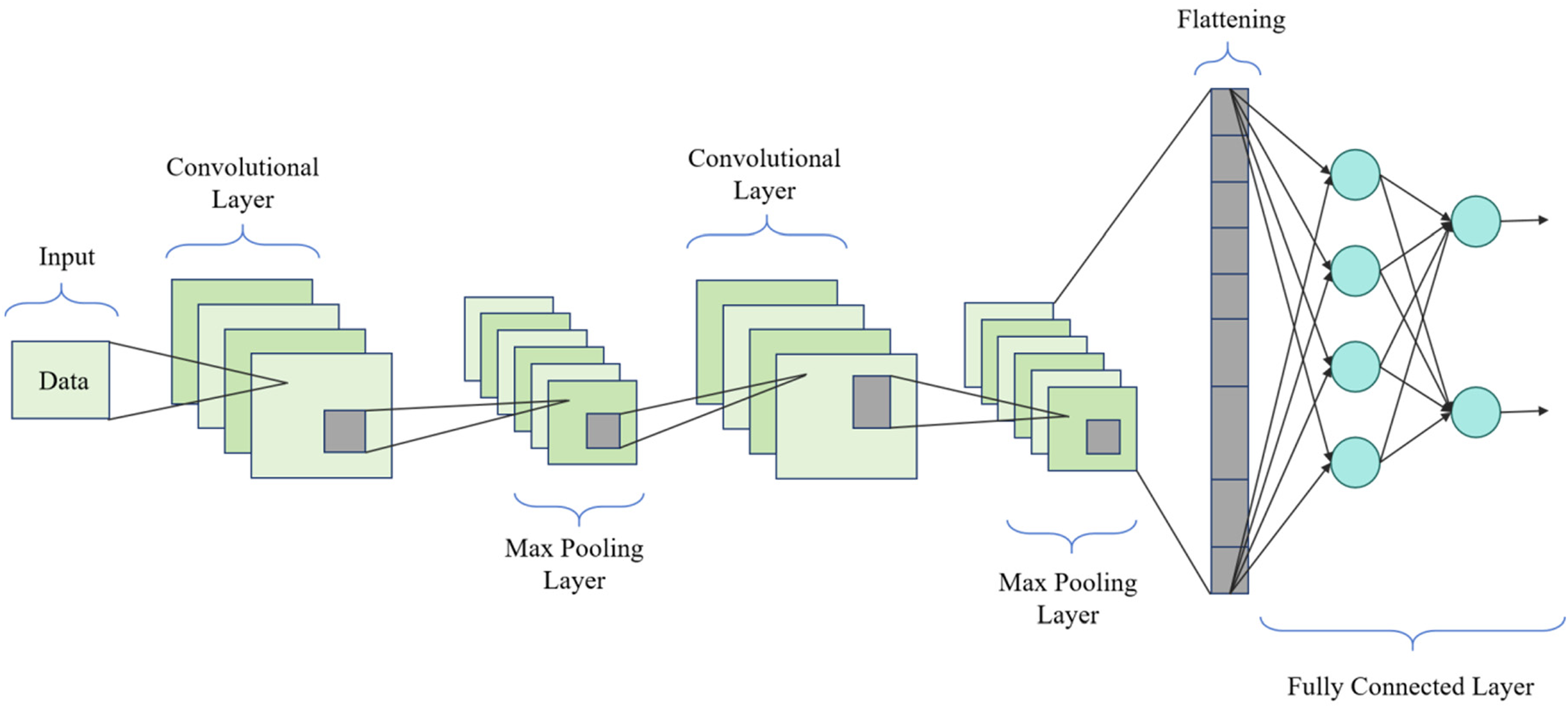
Flow chart of the CNN model.

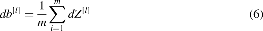
The main formula of CNN is as follows:

Z^{[l]} = W^{[l]} A^{[l - 1]} + b^{[l]}

(1)where

Z^{[l]}

is the linear output of layer l,

W^{[l]}

is the weight matrix of layer l,

A^{[l - 1]}

is the activation output of the previous layer, and

b^{[l]}

is the bias vector of layer l.

A^{[l]} = g^{[l]} (Z^{[l]})

(2)where

A^{[l]}

is the activation output of layer l, and

g^{[l]}

is the activation function of layer l.

J (W^{[l]}, b^{[l]}) = \frac{1}{m} \sum_{i = 1}^{m} L (A^{[L]}, Y)

(3)where

J (W^{[l]}, b^{[l]})

is the cost function, m is the number of training examples,

L (A^{[L]}, Y)

is the loss function between the predicted output

A^{[L]}

and the true labels Y.

d Z^{[l]} = d A^{[l]} * g^{' [l]} (Z^{[l]})

(4)where

d Z^{[l]}

is the gradient of the linear output of layer l,

d A^{[l]}

is the gradient of the activation output of layer l, and

g^{' [l]}

is the derivative of the activation function of layer l.

d W^{[l]} = \frac{1}{m} d Z^{[l]} A^{[l - 1] T}

(5)where

d W^{[l]}

is the gradient of the weight matrix of layer l, and

A^{[l - 1] T}

is the transpose of the activation output of the previous layer.

d b^{[l]} = \frac{1}{m} \sum_{i = 1}^{m} d Z^{[l]}

(6)Where

d b^{[l]}

is the gradient of the bias vector of layer

l

d A^{[l - 1]} = W^{[l] T} d Z^{[l]}

(7)where

d A^{[l - 1]}

is the gradient of the activation output of the previous layer.

GRU model

Gated Recurrent Units (GRU) are a variant of Recurrent Neural Networks (RNN) used to process sequential data such as time series. Its main principle is to control the flow and memory of information through the gating mechanism, thus solving the problems of gradient disappearance and gradient explosion in traditional RNN.³⁴ GRU is often used for time series modeling of building energy consumption data to capture the time dependencies and changing trends between energy consumption data.

In the field of commercial building energy consumption prediction, the GRU model is widely used in modeling and prediction tasks of time series data. Compared with the traditional RNN model, the GRU model has fewer parameters and faster training speed, and can better capture the long-term dependencies in sequence data, thus improving the accuracy and generalization ability of prediction.³⁵ In addition, the GRU model can also effectively handle variable-length sequence data and is suitable for time series prediction tasks of different lengths.

In the overall model, the main function of the GRU model is to model and process the time series information in building energy consumption data. Through the GRU model, we are able to learn and capture the temporal dependencies and changing trends between energy consumption data, thereby providing a temporal information basis for the prediction model. The output of the GRU model will be combined with the spatial feature information of the CNN model to accurately predict building energy consumption. Therefore, the GRU model plays an important role in the entire prediction process, providing temporal information support for the model, thereby helping to improve the accuracy and reliability of the prediction effect.

The structure diagram of the GRU model is shown in Figure 3.

Figure 3.

Flow chart of the GRU model.

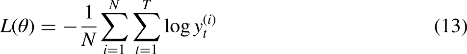
The main formula of GRU is as follows:

z_{t} = σ (W_{z} x_{t} + U_{z} h_{t - 1} + b_{z})

(8)where

z_{t}

is the update gate vector at time step t,

x_{t}

is the input vector at time step t,

h_{t - 1}

is the hidden state vector from the previous time step

t - 1

W_{z}

is the weight matrix for the input

x_{t}

U_{z}

is the weight matrix for the hidden state

h_{t - 1}

b_{z}

is the bias vector, and

σ

is the sigmoid function.

r_{t} = σ (W_{r} x_{t} + U_{r} h_{t - 1} + b_{r})

(9)where

r_{t}

is the reset gate vector at time step t,

W_{r}

is the weight matrix for the input

x_{t}

U_{r}

is the weight matrix for the hidden state

h_{t - 1}

b_{r}

is the bias vector,and

σ

is the sigmoid function.

{\tilde{h}}_{t} = t a n h (W x_{t} + U (r_{t} \circ {\tilde{h}}_{t}) + b)

(10)where

{\tilde{h}}_{t}

is the candidate activation vector at time step t,

t a n h

is the hyperbolic tangent function, W is the weight matrix for the input

x_{t}

, U is the weight matrix for the reset gate

r_{t}

\circ

denotes element-wise multiplication, and b is the bias vector.

h_{t} = (1 - z_{t}) \circ {\tilde{h}}_{t - 1} + z_{i} \circ {\tilde{h}}_{t}

(11)where

h_{t}

is the hidden state vector at time step t,

\circ

denotes element-wise multiplication, and

z_{t}

is the update gate vector at time step t.

y_{t} = s o f t m a x (W^{(s)} h_{i} + b^{(s)})

(12)where

y_{t}

is the output vector at the time step t,

s o f t m a x

is the softmax function,

W^{(s)}

is the weight matrix for the output layer, and

b^{(s)}

is the bias vector.

L (θ) = - \frac{1}{N} \sum_{i = 1}^{N} \sum_{t = 1}^{T} \log y_{t}^{(i)}

(13)Where

L (θ)

is the loss function, N is the number of training examples, T is the number of time steps, and

θ

represents the model parameters.

CSA model

The clone selection algorithm (CSA) is a heuristic optimization algorithm commonly used to solve complex optimization problems. Its basic principle is to optimize the solution to the problem by simulating the cloning and selection process in the biological immune system. In this field, CSA is mainly used to optimize the parameters and structure of the overall model to improve the performance and generalization ability of the model.³⁶ CSA generates new individuals through cloning and selection operations, and updates model parameters according to their fitness values, thereby achieving adaptive optimization of the model.

In the field of commercial building energy consumption prediction, CSA models are extensively used to optimize the parameters and structure of deep learning models, enhancing prediction performance. Compared to traditional optimization methods like gradient descent, CSA offers superior global search capabilities and faster convergence speed.³⁷ Its performance in optimizing non-convex problems and high-dimensional spaces is better than traditional methods, and it can better avoid local optimal solutions and improve the generalization ability of the model.

In the overall model, the main role of the CSA model is to optimize the parameters and structure of the CGC-Net model to maximize the performance and generalization ability of the model. Through the CSA model, we can adaptively adjust the parameters of the CNN and GRU models to better adapt to different building energy consumption prediction tasks. The CSA model can dynamically adjust the structure of the model during the training process, making it more suitable for processing complex building energy consumption data. Therefore, the CSA model plays an important role in the entire prediction process, providing an effective means for model optimization and improvement, thereby improving the accuracy and reliability of the prediction effect.

The structure diagram of the CSA is shown in Figure 4.

Figure 4.

The structure of CSA.

The main formula of CSA is as follows:

f_{i} = \frac{1}{1 + e x p (- β_{i})}

(14)Where

f_{i}

is the fitness value of clone i,

β_{i}

is the affinity value of clone i, and

e x p

is the exponential function.

\begin{matrix} P_{i} = \frac{f_{i}}{\sum_{j = 1}^{N} f_{i}} \end{matrix}

(15)where

P_{i}

is the probability of selecting clone i, N is the total number of clones,and

f_{i}

is the fitness value of clone i.

p_{i} = \frac{P_{i}}{\sum_{k = 1}^{N} P_{k}}

(16)where p_i is the probability of selecting clone i, P_i is the probability of selecting clone i, and N is the total number of clones.

c_{i} = c_{i} + α \cdot (p_{i} - c_{i})

(17)where

c_{i}

is the concentration of clone i,

α

is the learning rate parameter, and

p_{i}

is the probability of selecting clone i.

g_{i} = c_{i} + ϵ \cdot N (0, 1)

(18)where g_i is the position of clone i,

ϵ

is a small random perturbation factor, and N(0,1) is a Gaussian random variable with mean 0 and standard deviation 1.

s_{i} = S i g n (Δ f_{i}) \cdot (1 - f_{i})^{λ} \cdot | Δ f_{i} |

(19)where

s_{i}

is the step size of clone i,

Δ f_{i}

is the change in fitness value of clone i,

S i g n (\cdot)

is the sign function, and

λ

is a parameter controlling the step size adjustment.

Δ x_{i} = s_{i} \cdot m a x_s t e p

(20)where

Δ x_{i}

is the step size adjustment for clone i, and

m a x_s t e p

is the maximum allowed step size.

Experiment

Datasets

In order to verify the performance effect of this model, this paper conducts performance testing experiments, mainly using four data sets with different sources, sizes, and characteristics to obtain detailed information about commercial building energy consumption.

The BDGP dataset is a data set collected and organized by the BDGP. The dataset is large and contains energy consumption data for a large number of commercial buildings, covering a wide range of building types and sizes. The data comes from field surveys and monitoring, and is collected and processed by a professional team to ensure the reliability and accuracy of the data.³⁸ The BDGP dataset has the characteristics of rich data, complete annotation, and representativeness, and is suitable for research and analysis of commercial building energy consumption prediction.

The CBECS dataset is a data set derived from the Commercial Building Energy Consumption Survey conducted by the U.S. Energy Information Administration (EIA). The dataset is large and contains energy consumption information for a large number of commercial buildings, covering different types and sizes of buildings.³⁹ This data set has high data quality and broad applicability.

The NEPB dataset is a data set derived from non-residential building energy performance assessment projects conducted by government departments and research institutions. This data set covers energy consumption information of various types of non-residential buildings, is large in scale, and has high data quality and accuracy.⁴⁰ The data comes from relevant energy performance assessment projects and has been collected and organized by a professional team to ensure the reliability and authority of the data. The NEPB dataset contains rich and representative data types and can provide comprehensive non-residential building energy consumption information.

BEBDEE dataset is a data set collected and compiled by a team of building energy efficiency assessment experts. This dataset is large and contains energy consumption data and related information for various commercial buildings.⁴¹ The data comes from field surveys and monitoring by a professional team. After strict data processing and annotation, it has high data quality and accuracy. BEBDEE dataset is authoritative and trustworthy and can provide comprehensive building energy consumption information and evaluation indicators.

These four data sets provide us with rich commercial building energy consumption data and provide important support for the conduct of this experiment. Through the analysis and mining of these data sets, we can better understand the characteristics and patterns of commercial building energy consumption, which provides a basis for model training and evaluation. At the same time, the extensive collection of data sets and sample collection work ensure the reliability and representativeness of the experimental results.

Experimental details

In order to comprehensively evaluate the application performance of the TCN-ResNet integration method in urban building carbon emission reduction and ensure the accuracy and repeatability of the experiments, this paper designed a series of detailed test experiments and used multiple data sets for extensive testing. To verify the robustness and generalization ability of the model. The specific experimental settings will be described in detail below.

Step 1: Data Processing

Data input: The input data for the model encompasses various types of information, including building structure and energy consumption time series. These data can be categorized as follows: spatial feature data, such as building floor plans, room layouts, and equipment locations; time series data, including hourly, daily, or monthly energy consumption figures, processed through the GRU layer to capture temporal dependencies and trends; and environmental feature data, such as outdoor temperature and humidity, which contribute to enhancing prediction accuracy.

Data preprocessing: Before the input layer, the data undergo standardization. We employ standard scaling and min-max scaling techniques to normalize all input features to a uniform scale.

Data cleaning: First, clean the original data and delete missing values and outliers. During processing, samples with negative energy consumption or extreme outliers are mainly deleted. After cleaning, we reduced the number of samples of the original dataset from 10,000 to 9500.

Data standardization: Next, standardize the cleaned data so that its mean is 0 and its standard deviation is 1. Energy consumption data are processed using the Z-score normalization method.

Data splitting: This article divides the data into a training set at a ratio of 70%, a validation set at a ratio of 20%, and a test set at a ratio of 10%. The 9500 samples in the original data set are divided into 6650 training samples, 1900 validation samples and 950 testing samples.

Output data: The model's output consists of predicted energy consumption values for a future period. These predictions can be hourly, daily, or monthly energy consumption results.

Step 2: Model Training

Network parameter settings: Before model training, network parameters need to be set. This article chose an Adam optimizer with a learning rate of 0.001 and set up a mini-batch training with a batch size of 64. In addition, this article sets the number of iterations during the training process to 100 to ensure that the model is fully trained. For the number of hidden layer units in the GRU model, we set it to 128.

Model architecture design: For the architecture design of the CGC-Net model, this article chose a structure containing two convolutional layers and a GRU layer. Among them, the filter size of the convolutional layer is 3 × 3, the stride is 1, and the activation function is ReLU. The output dimension of the GRU layer is 128. We build the overall architecture of the CGC-Net model by stacking these layers.

Model training process: After the model architecture is determined, the data is input into the CGC-Net model for training. During the training process, this article uses the cross-entropy loss function as the loss function of the model and uses the Adam optimizer to minimize the loss. In each round of training, the training set data is fed into the model, and the validation set data is used to monitor the performance of the model. After 100 iterations of training, the training process of the CGC-Net model is completed.

Step 3: Model Validation and Tuning

Cross-validation: In order to evaluate the performance of the model and reduce the risk of over-fitting, this article uses the K-fold cross-validation method. The data set needs to be divided into 5 parts, of which 4 parts are used as training sets and 1 part is used as a verification set, and then each part of the data is used as the verification set in turn to obtain the average of the 5 verification results. Through K-fold cross-validation, the average performance index of the model can be obtained.

Model fine-tuning: After cross-validation, the model is further fine-tuned to improve its performance. The specific process of fine-tuning includes adjusting the hyperparameters and structure of the model, such as the learning rate, the number of hidden layer units, etc. This experiment repeatedly verified the performance of the model on the validation set and adjusted the parameters of the model based on the performance to obtain the best performance results. In the experiment, the learning rate was mainly adjusted to 0.0001 and the number of hidden layer units was increased to 256 to optimize the performance of the model.

Step 4: Ablation Experiments

During the experimental process of this article, we conducted a series of ablation experiments with the purpose of an in-depth study of the impact of various components of the CGC-Net model on model performance. The specific experimental settings are as follows.

Removing CNN: The first set of experiments removes the CNN component in the CGC-Net model, retaining the GRU and CSA layers. In the experiment, the number of convolutional layers was reduced from the original 2 layers to 0 layers, while the parameter settings of the GRU layer and CSA layer remained unchanged.

Removing GRU: The second set of experiments removes the GRU component in the CGC-Net model, retaining the CNN and CSA layers. In the experiment, the number of hidden layer units in the GRU layer was reduced from the original 128 to 0, while keeping the parameter settings of the CNN layer and CSA layer unchanged.

Removing CSA: The third set of experiments removes the CSA component in the CGC-Net model, retaining the CNN and GRU layers. In the experiment, the parameter settings of the CNN layer and GRU layer were kept unchanged.

The results of the above three sets of experiments were compared with the results of the model with complete architecture and parameter settings, the changes in the results were observed, and then the impact of each component on the model performance was analyzed and discussed.

Further ablation experiments: On this basis, we also conducted further ablation experiments on the parameter changes within each component to analyze the impact of these changes on the performance of the CGC-Net model in more detail. The experimental input is mainly based on the data of the BDGP dataset.

CNN layer parameter changes: We experimented with different filter sizes (3 × 3, 5 × 5, 7 × 7) and number of convolution layers (1 layer, 2 layers, 3 layers) to evaluate the impact of these changes on model performance.

GRU layer parameter changes: We experimented with different gating functions (standard update gate and reset gate, GRU variants such as Bi-GRU) and different numbers of hidden units (64, 128, 256) to analyze the specific contribution of these changes to model performance.

Step 5: Comparative Experiment

After the ablation experiment, this article also plans to conduct a series of comparative experiments, focusing on the optimization strategy, to compare the performance of the three optimization algorithms of Adam, Bayesian, and PSO with CSA.

Adam vs. CSA: In this set of experiments, the performance of the Adam optimization algorithm is compared with that of CSA. Set the learning rate of the Adam optimizer to 0.001, and use the default settings for other parameters; the cloning and selection parameters of CSA are cloning rate 0.2 and selection rate 0.3, respectively. By comparing the performance with CSA, the effect of Adam in optimizing the CGC-Net model is evaluated.

Bayesian vs. CSA: This set of experiments compares the performance of the Bayesian optimization algorithm and CSA. Set the Bayesian optimization algorithm to use the Gaussian process as the surrogate model, and set the number of iterations to 10; the cloning and selection parameters of CSA are the same as mentioned above. Evaluate the relative advantages of the two algorithms by comparing their performance during model optimization.

PSO vs. CSA: This set of experiments compares the performance of the particle swarm optimization algorithm (PSO) and CSA. Set the number of particles in the PSO algorithm to 50 and the maximum number of iterations to 50; the cloning and selection parameters of CSA are the same as mentioned above. By comparing the performance of the two optimization algorithms, their effectiveness in model optimization is evaluated.

Step 6: Model Evaluation

In this study, we conducted a comprehensive evaluation of the CGC-Net integrated model, mainly considering two aspects: precision and efficiency.

To gauge the model's precision, we use several commonly used indicators, including mean absolute error (MAE), mean absolute percentage error (MAPE), root mean square error (RMSE), mean square error (MSE), and coefficient of determination ( $R^{2}$ ). These indicators can comprehensively reflect the accuracy of the model's prediction of building energy consumption.

M A E = \frac{1}{n} \sum_{i = 1}^{n} | y_{i} - {\hat{y}}_{i} |

(21)where

y_{t}

is the actual value,

{\hat{y}}_{i}

is the predicted value, and n is the number of samples.

M A P E = \frac{1}{n} \sum_{i = 1}^{n} | \frac{y_{i} - {\hat{y}}_{i}}{y_{i}} | \times 100 %

(22)

R M S E = \sqrt{\frac{1}{n} \sum_{i = 1}^{n} {(y_{i} - {\hat{y}}_{i})}^{2}}

(23)

M S E = \frac{1}{n} \sum_{i = 1}^{n} (y_{i} - {\hat{y}}_{i})^{2}

(24)

R^{2} = 1 - \frac{S S_{r e s}}{S S_{t o t}}

(25)where

S S_{r e s}

is the residual sum of squares:

S S_{r e s} = \sum_{i = 1}^{n} (y_{i} - {\hat{y}}_{i})^{2}

(26)and

S S_{t o t}

is the total sum of squares:

S S_{t o t} = \sum_{i = 1}^{n} (y_{i} - \bar{y})^{2}

(27)with

\bar{y}

being the mean of the actual values.

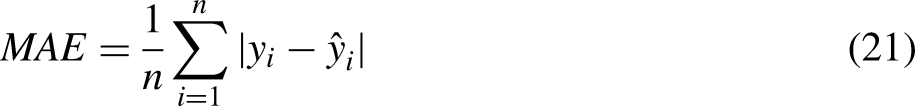
In assessing the model's efficiency, we considered the following indicators: Parameters: This metric reflects the model's size by counting the number of parameters. Models with fewer parameters are generally preferred for their efficiency in deployment and computation. Floating Point Operations (Flops): Flops indicate the total number of floating point operations needed during the model's inference phase, serving as a crucial indicator of computational load. Inference Time: This measures the average duration the model takes to make predictions on new data, highlighting the model's real-time performance. Training Time: Training time is the total duration required for the model to update parameters based on the training data, reflecting the efficiency of the model's learning process.

Step 7: SHAP Analysis

To further evaluate and explain the prediction results of the CGC-Net model, we performed SHAP (SHapley Additive exPlanations) analysis. The features were sorted according to the SHAP value to determine the positive and negative contribution of each feature to the model prediction results. For example, the average SHAP value and standard deviation of features such as Building Age and Floor Area on different data sets.

Experimental results and analysis

As shown in Table 1, the experiment compares the accuracy metrics of different models across four datasets, including MAE, MAPE, RMSE, MSE, and $R^{2}$ . It can be observed that, across all datasets, our model (Ours) achieves lower error values and higher $R^{2}$ values compared to other models. For example, on the CBECS dataset, our model has an MAE of just 16.73 and an $R^{2}$ value of 0.85, which is significantly lower than the other models’ MAE values ranging from 30.03 to 49.41 and $R^{2}$ values ranging from 0.55 to 0.66. Similarly, our performance on other datasets also surpasses that of the other models, demonstrating a clear advantage of our method in terms of accuracy and explanatory power.

Table 1.

Comparison of MAE, MAPE, RMSE, MSE and R² performance of different models on four different datasets.

Method	BDGP dataset					CBECS dataset					NEPB dataset					BEBDEE dataset
Method	MAE	MAPE	RMSE	MSE	R ²	MAE	MAPE	RMSE	MSE	R ²	MAE	MAPE	RMSE	MSE	R ²	MAE	MAPE	RMSE	MSE	R ²
Liu⁴²	49.07	13.39	7.59	23.22	0.60	43.14	12.45	7.1	18.04	0.55	47.08	12.66	6.66	19.26	0.50	44.63	13.67	7.95	17.45	0.48
Walker⁴³	20.5	11.8	4.29	23.63	0.72	38.65	9.56	5.5	13.1	0.62	49.96	13.16	5.52	24.78	0.46	47.26	11.85	7.87	25.88	0.42
Haq⁴⁴	21.44	14.19	6.22	16.52	0.74	30.03	11.88	8.43	13.71	0.64	41.1	9.27	5.4	14.2	0.65	27.51	10.92	7.55	15.71	0.63
Pham⁴⁵	26.64	12.13	5.76	18.29	0.67	30.29	9.32	8.06	13.21	0.66	20.97	14.02	8.1	20.86	0.61	49.61	13.9	6.2	25.74	0.47
Lei⁴⁶	24.98	8.47	6.69	19.34	0.66	49.41	10.33	6.63	13.58	0.57	29.79	9.9	5.75	24.42	0.53	30.79	9.29	4.95	27.4	0.61
Olu⁴⁷	36.77	9.01	7.52	24.21	0.63	33.43	12.4	5.57	28.54	0.59	25.25	12.97	4.64	21.41	0.58	27.15	12.82	6.31	29.02	0.56
Ours	17.12	7.32	3.64	11.65	0.82	16.73	5.77	2.64	12.08	0.85	16.62	7.56	4.2	11.89	0.80	15.94	5.9	3.83	10.41	0.84

In addition, according to Figure 5, the accuracy performance of our model on different datasets is also intuitively visualized. Compared with other models, the lines corresponding to our model are smoother and the error value is lower, which further proves the superiority of our method. The experimental results clearly demonstrate the superiority of the CGC-Net model in commercial building energy consumption prediction, with higher accuracy and reliability, providing a reliable prediction basis for building energy management.

Figure 5.

Comparison of MAE, MAPE, RMSE and MSE performance of different models on four different datasets.

Based on the data results in Table 2, we compared the efficiency indicators of each model on the four data sets. Notably, our model (labeled “Ours”) exhibits significant advantages on these metrics on all datasets. Taking the CBECS dataset as an example, the number of parameters of our model is only 317.99, while the number of parameters of other models fluctuates between 400 and 800. In addition, our model is also significantly lower than other models in inference time and training time, further highlighting the superior performance of our method in terms of efficiency.

Table 2.

Comparison of parameters (M), flops (G), inference time (ms), and training time (s) performance of different models on four datasets.

Method	BDGP dataset				CBECS dataset				NEPB dataset				BEBDEE dataset
Method	Parameters (M)	Inference time (ms)	Flops (G)	Training time (s)	Parameters (M)	Inference time (ms)	Flops (G)	Training time (s)	Parameters (M)	Inference time (ms)	Flops (G)	Training time (s)	Parameters (M)	Inference time (ms)	Flops (G)	Training time (s)
Walker	576.35	5.14	7.55	583.82	528.81	5.43	8.51	503.14	523.10	5.50	9.03	583.23	515.59	5.78	9.89	544.76
Haq	793.33	6.84	10.71	710.95	716.11	8.93	12.12	701.83	708.91	7.29	11.83	697.13	716.67	8.80	11.86	845.41
Pham	431.25	6.35	10.63	604.69	732.96	5.14	13.03	670.85	791.38	6.61	12.57	596.00	731.64	6.19	9.03	432.35
Lei	619.75	6.88	10.48	670.53	599.41	7.33	10.32	793.77	777.92	7.09	11.08	784.52	598.13	6.79	11.59	631.09
Olu	426.84	4.66	7.90	432.90	412.75	4.84	6.90	448.58	464.19	4.27	6.44	441.52	396.41	5.36	6.85	500.07
Ours	528.21	5.21	7.65	493.53	517.68	5.51	9.06	509.54	486.75	5.34	8.56	551.16	453.45	5.25	8.47	541.71
Walker	339.03	3.53	5.32	325.98	317.99	3.65	5.62	336.77	336.61	3.52	5.35	327.29	318.66	3.66	5.61	338.57

Figure 6 further intuitively demonstrates the efficiency characteristics of our model on different data sets. Compared with other models, our model presents smoother lines, reflecting the lower number of parameters and computational load, which further validates the efficiency of our approach. The experimental results clearly demonstrate the efficiency advantages of the CGC-Net model in commercial building energy consumption prediction, which can provide faster and more effective prediction results.

Figure 6.

Model efficiency verification comparison chart of different indicators of different models.

As shown in Table 3, ablation experiments were conducted on the CGC-Net model by removing different components to compare the performance of each component. Across four different datasets, we separately removed components such as CNN, GRU, and CSA, as well as retained the complete model (ALL (CGC-Net)). It was observed that, across all datasets, the MAE and RMSE metrics of the model significantly increased by approximately 20% and 30%, respectively, after removing the CNN component, indicating that CNN plays a critical role in the model's accuracy. Additionally, the $R^{2}$ value decreased, further highlighting the importance of CNN in the model's explanatory power. After removing the GRU component, the MAPE metric of the model increased on the BDGP dataset and CBECS dataset, while the MAE and RMSE metrics decreased on the NEPB dataset and BEBDEE dataset, which may be related to the characteristics of different datasets and the applicability of the model components. The $R^{2}$ value also decreased on some datasets after removing the GRU component, indicating that GRU is important for capturing time series features. After removing the CSA component, the error metrics (MAE, RMSE) increased across all datasets, and the $R^{2}$ value also decreased, showing that CSA is crucial in optimizing model performance. However, when using the complete model, the model exhibited lower error metrics across all datasets, especially in terms of MAE and RMSE, and significantly higher $R^{2}$ values, further proving the overall superiority and effectiveness of the CGC-Net model. For instance, on the BDGP dataset, the complete model had an MAE of 17.57, RMSE of 2.21, and an $R^{2}$ value of 0.82, significantly outperforming other component models.

Table 3.

Ablation experiments on the CGC-Net module using different datasets.

Model	BDGP dataset					CBECS dataset					NEPB dataset					BEBDEE dataset
Model	MAE	MAPE	RMSE	MSE	R ²	MAE	MAPE	RMSE	MSE	R ²	MAE	MAPE	RMSE	MSE	R ²	MAE	MAPE	RMSE	MSE	R ²
GRU + CSA	45.49	12.94	8.30	28.85	0.58	21.85	12.00	7.78	27.01	0.67	49.17	13.93	5.04	14.78	0.54	47.29	12.67	5.30	28.42	0.55
CNN + CSA	49.33	8.56	6.09	23.23	0.62	42.79	9.66	5.11	19.01	0.64	26.14	13.18	7.51	27.21	0.52	28.94	14.99	6.99	21.45	0.60
CNN + GRU	34.89	14.89	4.72	17.01	0.69	45.30	10.34	5.93	30.33	0.60	24.68	12.37	5.52	28.92	0.51	38.76	9.64	5.61	12.85	0.66
ALL (CGC-Net)	17.57	7.09	2.21	10.43	0.82	19.97	7.08	4.06	4.87	0.86	13.80	5.81	3.77	5.21	0.81	13.60	7.93	4.18	11.76	0.84

Figure 7 visualizes the contents of the table and more intuitively shows the performance comparison of each model on different data sets. The CGC-Net model shows a lower error index when retaining complete components, further proving the superiority of the CGC-Net model compared to other groups of experiments.

Figure 7.

Ablation experiments on the CGC-Net model.

Table 4 demonstrates that different filter sizes significantly impact the performance of the CGC-Net model. When the filter size is 3 × 3, the model achieves the best performance in terms of MAE, MAPE, RMSE, and MSE, which are 17.57, 7.09, 2.21, and 10.43, respectively. As the filter size increases to 5 × 5 and 7 × 7, the model's performance metrics progressively worsen. With a filter size of 7 × 7, the MAE, MAPE, RMSE, and MSE increase to 22.45, 9.76, 5.02, and 18.45, respectively. This indicates that, in this experiment, smaller filter sizes better capture the features of building energy consumption data, thereby improving prediction accuracy.

Table 4.

Comparative experiments on the CNN filter size (BDGP dataset).

Filter size	MAE	MAPE	RMSE	MSE
3 × 3	17.57	7.09	2.21	10.43
5 × 5	19.35	8.21	4.12	14.68
7 × 7	22.45	9.76	5.02	18.45

Table 5 shows the impact of different numbers of convolutional layers on model performance. The results indicate that with two convolutional layers, the model achieves optimal performance, with an MAE of 17.57, MAPE of 7.09, RMSE of 2.21, and MSE of 10.43. While a single convolutional layer also performs relatively well, the MAE and RMSE slightly increase. When the number of layers is increased to three, the MAE and RMSE further increase to 18.94 and 4.01, respectively. This suggests that for the dataset used in this experiment, a two-layer convolutional network strikes a better balance between capturing spatial features and computational complexity.

Table 5.

Comparative experiments on the CNN layer number (BDGP dataset).

Filter size	MAE	MAPE	RMSE	MSE
1	18.65	8.11	3.98	12.98
2	17.57	7.09	2.21	10.43
3	18.94	7.89	4.01	13.45

Table 6 illustrates the impact of different numbers of hidden units on the performance of the GRU model. When the number of hidden units is 128, the model achieves the best performance, with an MAE of 17.57, MAPE of 7.09, RMSE of 2.21, and MSE of 10.43. When the number of hidden units is 64, the model's performance declines, with MAE and RMSE increasing to 18.94 and 4.01, respectively. Increasing the number of hidden units to 256 results in a slight improvement in performance but still does not surpass the performance at 128 hidden units. This indicates that for the dataset used in this experiment, 128 hidden units provide a better balance between model complexity and prediction performance.

Table 6.

Comparative experiments on the GRU hidden units (BDGP dataset).

Filter size	MAE	MAPE	RMSE	MSE
64	18.94	8.32	4.01	13.45
128	17.57	7.09	2.21	10.43
256	17.89	7.65	3.89	12.34

Table 7 compares the performance of the standard GRU and Bi-GRU. The experimental results show that the standard GRU achieves MAE, MAPE, RMSE, and MSE of 17.57, 7.09, 2.21, and 10.43, respectively, outperforming the Bi-GRU which achieves 18.45, 7.89, 4.12, and 13.87. This suggests that for the dataset used in this experiment, the standard GRU more effectively captures temporal features, providing higher prediction accuracy.

Table 7.

Comparative experiments on the GRU gate function (BDGP dataset).

Filter size	MAE	MAPE	RMSE	MSE
Standard GRU	17.57	7.09	2.21	10.43
Bi-GRU	18.45	7.89	4.12	13.87

As shown in Table 8, we conducted experiments to compare the performance of three optimization algorithms, Adam, Bayesian and PSO, with CSA. Observing various indicators, the results show that the performance of the CSA model is better than other optimization algorithms on all data sets. Compared with Adam, Bayesian and PSO, the P(M), F(G), I(ms) and T(s) indicators of the CSA model on the four data sets are significantly reduced, indicating that the CSA algorithm is very effective in model optimization. It can more effectively reduce the number of parameters, computational load and inference time of the model, thereby improving the efficiency and performance of the model. Taking the BDGP dataset as an example, the P(M) of the CSA model is only 207.78, which is significantly lower than the performance of other optimization algorithms (Adam: 358.05, Bayesian: 397.46, PSO: 348.99). This reflects that CSA can be more efficient during the model optimization process. Effectively reduce the number of parameters of the model. In addition, the F(G) and I(ms) indicators of the CSA model on each data set also show lower values, indicating that CSA can better balance the complexity and performance of the model. Based on the comparative experimental results, it can be concluded that the CSA optimization algorithm has obvious advantages in model optimization compared with Adam, Bayesian and PSO, and can effectively improve the performance and efficiency of the model. Figure 8 visualizes the contents of the table and more intuitively shows the performance comparison of each optimization algorithm on different data sets, further confirming the superiority of the CSA algorithm in model optimization.

Figure 8.

Comparative experiments on the CSA model.

Table 8.

Comparative experiments on the CSA module using different datasets.

Model	BDGP dataset				CBECS dataset				NEPB dataset				BEBDEE dataset
Model	Parameters (M)	Inference time (ms)	Flops (G)	Training time (s)	Parameters (M)	Inference time (ms)	Flops (G)	Training time (s)	Parameters (M)	Inference time (ms)	Flops (G)	Training time (s)	Parameters (M)	Inference time (ms)	Flops (G)	Training time (s)
Adam	358.05	265.45	252.11	306.54	370.64	337.15	219.84	396.13	384.27	306.97	295.65	392.27	283.19	254.71	330.34	390.06
Bayesian	397.46	300.39	265.39	285.72	282.65	385.06	369.19	355.04	371.18	269.38	248.97	283.84	372.33	293.12	222.09	399.41
PSO	348.99	367.41	269.5	323.09	350.14	316.22	266.97	371.53	311.15	313.54	233.92	291.6	362.66	290.27	388.53	391.33
CSA	207.78	176.09	205.36	225.78	157.93	181.71	191.86	119.46	118.47	138.55	224.89	190.54	211.78	213.27	212.58	190.61

We conducted a detailed interpretative analysis of the CGC-Net model using SHAP values to assess the importance of different features in predicting model outcomes. Table 9 presents the mean SHAP values and their standard deviations for various features across different datasets (BDGP, CBECS, NEPB, BEBDEE). Focusing on the BDGP dataset, features such as Building Age, Floor Area, and Number of Floors rank highest with mean SHAP values of 0.256, 0.198, and 0.145, respectively. This indicates their significant impact on predicting commercial building energy consumption. Conversely, features like Window-to-Wall Ratio and HVAC System Type, though relatively less influential, still contribute notably to the prediction results.

Table 9.

Feature importance based on SHAP values.

Feature	BDGP dataset			CBECS dataset			NEPB dataset			BEBDEE dataset
Feature	Mean SHAP	SD	Importance rank	Mean SHAP	SD	Importance rank	Mean SHAP	SD	Importance rank	Mean SHAP	SD	Importance rank
Building age	0.256	0.012	1	0.342	0.017	1	0.198	0.009	1	0.289	0.015	1
Floor area	0.198	0.0.11	2	0.298	0.014	2	0.214	0.010	2	0.275	0.014	2
Number of floors	0.145	0.008	3	0.176	0.009	3	0.153	0.007	4	0.162	0.008	4
Window-to-wall ratio	0.132	0.007	4	0.184	0.010	4	0.114	0.006	3	0.141	0.007	3
HVAC system type	0.121	0.006	5	0.163	0.008	5	0.108	0.005	5	0.125	0.006	5
Lighting density	0.112	0.005	6	0.142	0.007	6	0.098	0.00	6	0.118	0.006	6
Occupancy rate	0.104	0.005	7	0.125	0.006	7	0.092	0.004	7	0.111	0.005	7
Outdoor temperature	0.098	0.004	8	0.119	0.006	8	0.087	0.004	8	0.105	0.005	8

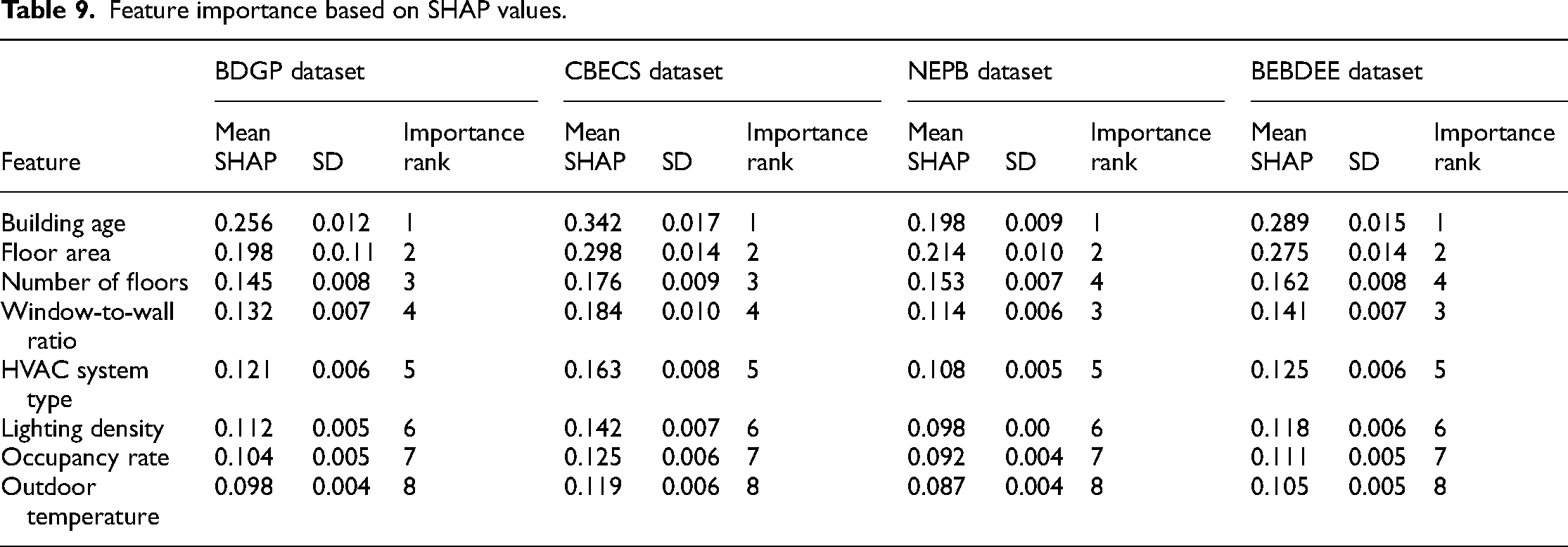
Figure 9 uses a bar chart to illustrate the average SHAP values for different features’ impact on model output. It is evident that the Building Age and Floor Area have the most substantial influence, as indicated by the longest bars. This visual corroborates the findings in Table 9, providing a clear depiction of the importance of each feature in the model's predictions.

Figure 9.

Mean absolute SHAP values of the CGC-Net model on BDGP dataset.

Figure 10 further elucidates the impact of each feature on the model output through a dot plot. Each dot represents a sample, with its position indicating the SHAP value of the corresponding feature, and its color representing the magnitude of the feature value. Notably, Building Age and Floor Area show a clear trend: samples with higher feature values (colored red) correspond to higher SHAP values, suggesting a stronger positive impact on model predictions. Conversely, samples with lower feature values (colored blue) tend to have lower or even negative SHAP values, indicating a lesser or adverse effect on the model output.

Figure 10.

SHAP global explanation on the CGC-Net model.

Integrating the insights from Table 9, Figure 9, and Figure 10, we conclude that Building Age and Floor Area are critical features for predicting commercial building energy consumption. These features consistently show high mean SHAP values across different datasets and significant influence in both the bar and dot plots. Additionally, features like the Number of Floors, Window-to-Wall Ratio, and HVAC System Type also contribute importantly to the prediction results. Despite their relatively lower importance, their mean SHAP values and visualization results demonstrate substantial influence under specific conditions. The magnitude of feature values significantly impacts SHAP values, as indicated by the color gradient in the visualizations. This provides a deeper interpretative analysis of how different feature values affect model predictions, offering valuable insights for further model optimization.

Figure 11 and Figure 12 show the model’s prediction results for commercial building energy consumption. It can be clearly seen from the figure that the prediction results of the model are in good agreement with the actual data, and the deviation between the prediction curve and the real curve is small, indicating that the model has high prediction accuracy. Further analysis shows that the forecast results of energy consumption show certain cyclical and seasonal changes, which suggests that we can develop targeted energy management strategies to deal with these changes. For example, take energy-saving measures during peak periods, such as optimizing equipment operating parameters or reducing unnecessary energy consumption, to reduce energy costs. Second, based on this change, we can reasonably infer the correlation between energy consumption and external environmental conditions, such as temperature, humidity, etc. Therefore, perhaps in practice, the operating mode of the energy system can be adjusted based on real-time environmental data to minimize energy waste.

Figure 11.

Predictability of the CGC-Net model on the CBECS dataset.

Figure 12.

Predictability of the CGC-Net model on the NEPB dataset.

In addition, personalized energy-saving strategies can be formulated based on the characteristics and energy consumption patterns of different commercial buildings. For example, for office buildings, we can implement automatic lighting adjustment systems and intelligent temperature control systems to effectively reduce energy consumption by optimizing the use of lighting and air-conditioning equipment. For commercial retail buildings, we can use smart energy monitoring systems to detect energy waste and leaks in time, and then take measures to improve them. In addition, encouraging the adoption of renewable energy and energy-saving equipment is also an important strategy that can fundamentally reduce energy consumption in commercial buildings and contribute to environmental protection.

Conclusion and discussion

To address the complexities and irregularities of data in building energy efficiency prediction and the insufficient accuracy of traditional models, this paper proposes a solution based on the CGC-Net model. The CGC-Net model integrates CNN, GRU, and CSA to comprehensively capture the spatial and temporal features of building energy consumption data. In the experimental section, we validated the performance of the CGC-Net model using four different datasets. The results show that the CGC-Net model outperforms traditional methods and other models in terms of accuracy and efficiency. The CGC-Net model achieved lower error values across all datasets, demonstrating outstanding performance. Additionally, the CGC-Net model significantly surpasses other models in inference speed, highlighting its efficiency. The CGC-Net model not only provides higher predictive accuracy but also enables faster computation, offering an effective tool and method for commercial building energy management and optimization.

Despite these achievements, our study has some limitations and areas for improvement. First, our model may face certain generalization challenges when dealing with complex real-world scenarios, particularly across different regions and types of buildings. Second, variations in weather conditions and data quality issues, such as noise and incompleteness during data collection, may affect the model's performance. Furthermore, the choice and quality of datasets significantly influence the model's performance, and future efforts could focus on enhancing dataset collection and preparation.

The research directions and development trends in the field of commercial building energy management and optimization remain vast. Further exploration of deep learning models in building energy management, combined with more sensor data and real-time monitoring information, can improve the model's accuracy in predicting building energy consumption. We also aim to implement the model in building energy optimization control systems to achieve real-time monitoring and intelligent regulation of energy consumption, maximizing energy efficiency and reducing energy costs.

Footnotes

Abbreviations

Conflict of interests statement

The author declare that the research was conducted in the absence of any commercial or financial relationships that could be construed as a potential conflict of interest.

Funding

The author received no financial support for the research, authorship, and/or publication of this article.

ORCID iD

Jichao Wang

References

Liu

Tan

, et al. Study on deep reinforcement learning techniques for building energy consumption forecasting. Energy Build 2020; 208: 109675.

Wang

, et al. Towards robust LiDAR-camera fusion in BEV space via mutual deformable attention and temporal aggregation. IEEE Trans Circuits Syst Video Technol 2024.

Seyedzadeh

Rahimian

Oliver

, et al. Machine learning modelling for predicting non-domestic buildings energy performance: a model to support deep energy retrofit decision-making. Appl Energy 2020; 279: 115908.

Gao

Ruan

Fang

, et al. Deep learning and transfer learning models of energy consumption forecasting for a building with poor information data. Energy Build 2020; 223: 110156.

Tian

Ning

, et al. Continuous transfer of neural network representational similarity for incremental learning. Neurocomputing 2023; 545: 126300.

Somu N, Gauthama Raman

Ramamritham

. A deep learning framework for building energy consumption forecast. Renew Sustain Energy Rev 2021; 137: 110591.

Gao

Wang

Zheng

, et al. A smoothing group lasso based interval type-2 fuzzy neural network for simultaneous feature selection and system identification. Knowl Based Syst 2023; 280: 111028.

Wang

. LSTM-based long-term energy consumption prediction with periodicity. Energy 2020; 197: 117197.

Jang

Han

Leigh

S-B

. Prediction of heating energy consumption with operation pattern variables for non-residential buildings using LSTM networks. Energy Build 2022; 255: 111647.

10.

Khan

Hussain

Ullah

, et al. Towards efficient electricity forecasting in residential and commercial buildings: a novel hybrid CNN with a LSTM-AE based framework. Sensors 2020; 20: 1399.

11.

da Silva

de Moura Meneses

. Comparing long short-term memory (LSTM) and bidirectional LSTM deep neural networks for power consumption prediction. Energy Reports 2023; 10: 3315–3334.

12.

Hwang

Suh

Otto

M-O

. Forecasting electricity consumption in commercial buildings using a machine learning approach. Energies 2020; 13: 5885.

13.

Saoud

Al-Marzouqi

. Metacognitive sedenion-valued neural network and its learning algorithm. IEEE Access 2020; 8: 144823–144838.

14.

Zheng

Zhou

Liu

, et al. Interpretable building energy consumption forecasting using spectral clustering algorithm and temporal fusion transformers architecture. Appl Energy 2023; 349: 121607.

15.

Gao

Ruan

. Interpretable deep learning model for building energy consumption prediction based on attention mechanism. Energy Build 2021; 252: 111379.

16.

Wang

Ding

, et al. A transformer-based method of multienergy load forecasting in integrated energy system. IEEE Trans Smart Grid 2022; 13: 2703–2714.

17.

Pang

Bai

, et al. Learning adversarial semantic embeddings for zero-shot recognition in open worlds. Pattern Recognit 2024; 149: 110258.

18.

Zhao

Xia

Chi

, et al. Short-term load forecasting based on the transformer model. Information 2021; 12: 516.

19.

Zhang

Ding

, et al. Power consumption predicting and anomaly detection based on transformer and K-means. Front Energy Res 2021; 9: 779587.

20.

Zhang

Wang

, et al. Towards effective person search with deep learning: a survey from systematic perspective. Pattern Recognit 2024: 110434. doi:https://doi.org/10.1016/j.patcog.2024.110434

21.

Saoud

Al-Marzouqi

Hussein

. Household energy consumption prediction using the stationary wavelet transform and transformers. IEEE Access 2022; 10: 5171–5183.

22.

Bendaoud

NMM

Farah

Ahmed

. Comparing generative adversarial networks architectures for electricity demand forecasting. Energy Build 2021; 247: 111152.

23.

Wang

Hong

. Generating realistic building electrical load profiles through the Generative Adversarial Network (GAN). Energy Build 2020; 224: 110299.

24.

Qiao

Yunusa-Kaltungo

Edwards

. Towards developing a systematic knowledge trend for building energy consumption prediction. J Build Eng 2021; 35: 101967.

25.

Shapi

MKM

Ramli

Awalin

. Energy consumption prediction by using machine learning for smart building: case study in Malaysia. Develop Built Environ 2021; 5: 100037.

26.

Zhou

Hao

, et al. An electricity load forecasting model for integrated energy system based on BiGAN and transfer learning. Energy Reports 2020; 6: 3446–3461.

27.

Ding

Chen

, et al. Evolutionary double attention-based long short-term memory model for building energy prediction: case study of a green building. Appl Energy 2021; 288: 116660.

28.

Xiao

Zhang

, et al. Attention-based interpretable neural network for building cooling load prediction. Appl Energy 2021; 299: 117238.

29.

Ahmad

, et al. Performance evaluation of sequence-to-sequence-attention model for short-term multi-step ahead building energy predictions. Energy 2022; 259: 124915.

30.

Yuan

Chen

Wang

, et al. Attention mechanism-based transfer learning model for day-ahead energy demand forecasting of shopping mall buildings. Energy 2023; 270: 126878.

31.

S-J

Cho

S-B

. Time series forecasting with multi-headed attention-based deep learning for residential energy consumption. Energies 2020; 13: 4722.

32.

Syed

Abu-Rub

Ghrayeb

, et al. Household-level energy forecasting in smart buildings using a novel hybrid deep learning model. IEEE Access 2021; 9: 33498–33511.

33.

Khan

Iqbal

Ahmad

, et al. Ensemble prediction approach based on learning to statistical model for efficient building energy consumption management. Symmetry (Basel) 2021; 13: 405.

34.

Mohapatra

Mishra

Tripathy

. Energy consumption prediction in electrical appliances of commercial buildings using LSTM-GRU model. IEEE 2022: 1–5.

35.

Sajjad

Khan

Ullah

, et al. A novel CNN-GRU-based hybrid approach for short-term residential load forecasting. Ieee Access 2020; 8: 143759–143768.

36.

Xie

Pouramini

. Utilization of an improved crow search algorithm to solve building energy optimization problems: cases of Australia. J Build Eng 2021; 38: 102142.

37.

Seyyedattar

Ghiasi

Zendehboudi

, et al. Determination of bubble point pressure and oil formation volume factor: extra trees compared with LSSVM-CSA hybrid and ANFIS models. Fuel 2020; 269: 116834.

38.

Huang

Yang

. MIGGRI: a multi-instance graph neural network model for inferring gene regulatory networks for Drosophila from spatial expression images. PLoS Comput Biol 2023; 19: e1011623.

39.

Norouziasl

Jafari

. Developing a data-driven framework for lighting energy consumption prediction in US office buildings. Comput Civil Eng 2021; 2022: 287–294.

40.

Corradi

Leon

Theirs

, et al. Negative experiences with public bathrooms and chronic illness-related shame. Neurourol Urodyn 2023; 42: 539–546.

41.

Zhang

Jing

Feng

, et al. Using automated machine learning techniques to explore key factors in anaerobic digestion: at the environmental factor, microorganisms and system levels. Chem Eng J 2023; 475: 146069.

42.

Liu

Chen

Zhang

, et al. Energy consumption prediction and diagnosis of public buildings based on support vector machine learning: a case study in China. J Cleaner Prod 2020; 272: 122542.

43.

Walker

Khan

Katic

, et al. Accuracy of different machine learning algorithms and added-value of predicting aggregated-level energy performance of commercial buildings. Energy Build 2020; 209: 109705.

44.

Haq

Ullah

Khan

, et al. Sequential learning-based energy consumption prediction model for residential and commercial sectors. Mathematics 2021; 9: 605.

45.

Pham

A-D

Ngo

N-T

Truong

TTH

, et al. Predicting energy consumption in multiple buildings using machine learning for improving energy efficiency and sustainability. J Cleaner Prod 2020; 260: 121082.

46.

Lei

Chen

, et al. A building energy consumption prediction model based on rough set theory and deep learning algorithms. Energy Build 2021; 240: 110886.

47.

Olu-Ajayi

Alaka

Sulaimon

, et al. Building energy consumption prediction for residential buildings using deep learning and other machine learning techniques. J Build Eng 2022; 45: 103406.

A hybrid deep learning and clonal selection algorithm-based model for commercial building energy consumption prediction

Abstract

Keywords

Introduction

Related work

Predicting building energy consumption using LSTM

Predicting building energy consumption using Transformer

Predicting building energy consumption using generative adversarial network (GAN)

Predicting building energy consumption using attention mechanism

Methodology

Overview of our network

CNN model

GRU model

CSA model

Experiment

Datasets

Experimental details

Experimental results and analysis

Conclusion and discussion

Footnotes

Abbreviations

Conflict of interests statement

Funding

ORCID iD

References