Sage Journals: Discover world-class research

Abstract

As one of the key parts of rotary machine, the fault diagnosis and running condition monitoring of rolling bearings are of great importance for normal working and safe production of rotary machine. However, the traditional diagnosis approaches merely count on artificial feature extraction and domain expertise. Meanwhile, the existing convolutional neural networks (CNNs) have the problem of low fault recognition rates. This paper proposes a novel convolutional neural network with one-dimensional structure (ODCNN) for the automatical fault diagnosis of rolling bearings, which adopts six sets of convolutional and max-pooling layers to extract signal features and applies a flattening convolutional layer followed by two fully-connected layers for feature classification. The architectures of one-dimensional LeNet-5, AlexNet, and the proposed ODCNN are illustrated in detail, followed by the obtaining of training and testing samples, which is pre-processed by overlapping the vibration signals of rolling bearings. Finally, the classification experiment is carried out. The experimental results show that the ODCNN has higher fault diagnosis rates and can achieve high accuracy with load variant. Additionally, the extracted features of three CNNs are visualized, which illustrate that the new CNN has a better classification capacity.

Keywords

Condition monitoring convolutional neural network (CNN)intelligent fault diagnosis deep learning rolling bearings

Introduction

As a pivotal part of mechanical equipment, the running and health status of rolling bearings has a vital impact on the performance of machines.¹ However, the working environment of rolling bearings is often accompanied by high temperature, high running speed, and complex alternating external loads, which makes them very vulnerable to failure.² Therefore, the fault diagnosis and condition monitoring of rolling bearings are of great significance to ensure the normal operation and safe production.

The procedure of traditional fault diagnosis ways mainly contains the extraction, selection, and classification of features from the bearing vibration signals.³ In the stage of feature extraction, the features that related to fault characteristics is extracted from original vibration signals for subsequent fault recognition. Correspondingly, the features of rolling bearings vibration signals can be extracted from frequency domain, time domain, and time-frequency domain.⁴ The statistical approaches⁵ such as Root Mean Square (RMS)⁶ and Kernel Density Estimation (KDE)⁷ are usually used in time domain; the Fast Fourier Transform (FFT) is often used for frequency domain analysis⁸; while for the time-frequency analysis, the most popular ways are Short-Time Fourier Transform (STFT) method,⁹ Wavelet Packet Transform (WPT),¹⁰ Empirical Mode Decomposition (EMD),¹¹ and its variations.¹² After feature extraction, the feature selection has to be carried out to remove the insensitive and useless features. The commonly used methods include Principal Component Analysis (PCA)¹³ and Independent Component Analysis (ICA).¹⁴ Finally, in the step of feature classification, the Artificial Neural Network (ANN) algorithms,¹⁵ k-Nearest Neighbor (kNN) method,¹⁶ and Support Vector Machine (SVM) approach¹⁷ are often employed to realize the classification of fault types. The traditional artificial approaches have been widely used for fault diagnosis of rolling bearings. However, there are several issues on the application of these methods: (1) the extraction of fault features is difficult and the classification accuracy depends on the signal processing techniques, relying on cumbersome artificial extraction and solid domain expertise¹⁸; (2) the coupling relationship among signal pretreatment, feature extraction and fault classification in the procedure of fault diagnosis is destroyed by human isolation, resulting in the loss of fault information partially.¹⁹

Contrast to traditional fault diagnostic methods, the deep learning method is a developing artificial intelligence technique, which can directly learn the diagnostic information in the vibration signals without any tedious denoising preprocessing and artificially extracting features. By using the structure of deep convolution neural network (CNN), the deep learning scheme is an end-to-end diagnostic method, which can combine feature extraction and feature classification into one step. Wen²⁰ discussed a novel CNN which extends from the LeNet-5 network structure and converted the vibration signals to 2D images as input to extract the features of rolling bearings. Hoang²¹ transformed the vibration signals of bearings into gray-scale images and used them as input data of the proposed CNN to detect bearing faults, and finally concluded that this approach can achieve very high accuracy and robustness under noisy environments. However, the bearing vibration data collected by accelerometer are only related to one-dimensional time, and data points at each time have spatio-temporal correlation. If they are directly converted into two-dimensional form, the spatial correlation in the original vibration signals will be destroyed, which may lead to the loss of information related to the faults.²² Therefore, some researchers attempt to construct one-dimensional CNNs, and try to use the original raw vibration signals as the input of CNNs directly. Janssens²³ proposed a shallow CNN model, which only consists of one convolutional layer with wide kernels followed by a fully connected layer, to monitor the rolling bearing health condition. In order to realize the intelligent fault diagnosis of rolling bearings, Sadoushi²⁴ presented a novel CNN that the signal processing is treated as the first layer, and the performance comparative study among deep learning-based methods, this new CNN and traditional machine learning is implemented. Zhang²⁵ proposed a 5-layer CNN to detect faults of rolling bearings, in which kernels in the first convolutional layer are wide while in the following layers are narrow. However, these approaches do not suitable for the condition of load variant and the fault recognition rates are not gratifying.

In order to further improve the fault diagnosis ability of rolling bearings, this paper investigate a new one-dimensional convolutional neural network (ODCNN). The rest of this paper is organized as follows. The net architectures and parameters of one-dimensional LeNet-5 (1D-LeNet-5), one-dimensional AlexNet (1D-AlexNet), and the proposed ODCNN is presented in Section 2. The experimental apparatus is introduced and the vibration signals of rolling bearings are pre-processed by overlapping segments to achieve samples for training and testing in Section 3. Finally, the classification accuracy is calculated and feature visualization technique is carried out to compare the classification capacity of three approaches before conclusions are drawn in Section 5.

Theory of CNN

The classical CNN consists of Convolutional layer, pooling layer and fully connected layer. In this section, the theory of the CNN is introduced in details.

Convolutional layer

The convolution layer is the core structure of CNN and its function is to extract different features of signal through different observation modes (also called convolution kernel) to realize the observation of specific mode of input signal. In order to extract different features from the input signal, a convolution layer usually has several convolution kernels, and different convolution kernels are used for convolution operation. Since the same convolution kernel shares parameters in the process of convolution, a convolution kernel learns a class of features called feature map. The convolution operation is defined as follows:

g (i) = \sum_{x = 1}^{m} \sum_{y = 1}^{n} \sum_{z = 1}^{p} a_{x, y, z} * w_{x, y, z}^{i} + b^{i}

(1)

where a is the input data, b is the offset of the convolution kernel, * is the convolution operation, i is the ith convolution kernel, and g(i) is the map obtained after the convolution operation of the ith convolution kernel. x, y and z represent the three-dimensional vectors of the signal. As the dimension of the bearing vibration signal is one-dimensional in this paper, the convolution operation can be expressed as follows:

g (i) = \sum_{x = 1}^{m} a_{x} * w_{x}^{i} + b^{i}

(2)

In order to avoid the problem of insufficient expression ability of linear model, the activation function is used for nonlinear transformation to filter the features obtained from the convolution operation. The commonly used sigmoid and tanh activation functions in the traditional neural network appear gradient disappearance phenomenon easily, resulting in the structure of network cannot be deepened. In recent years, the unsaturated nonlinear function Relu (rectified linear units) has been widely applied into the CNN as activation function, which has faster convergence speed than the traditional saturated nonlinear function when the training gradient drops. The expression of Relu activation function is as follows

f (i) = H (g (i)) = max {0, g (i)} i = 1, 2, \dots, q

(3)

where f(i) is the activation value of g(i) mapped by Relu function.

Pooling layer

The purpose of pooling layer is to reduce the number of neurons in the network through pooling operation. After pooling operation, the number of connections between convolution layers is reduced and the calculation speed is accelerated. The commonly used pooling methods are maximum pooling (taking the point with the maximum value in the local acceptance domain) and average pooling (averaging all values in the local acceptance domain). They can be defined as follows

P_{i}^{l + 1} (j) = max_{(j - 1) W + 1 \leq t \leq jW} {q_{i}^{l} (t)}

(4)

P_{i}^{l + 1} (j) = \underset{(j - 1) W + 1 \leq t \leq jW}{average} {q_{i}^{l} (t)}

(5)

where, W is the width of the pool area; $q_{i}^{l} (t)$ represents the value of the tth neuron in the ith eigenvector of the lth layer, and $t \in [(j - 1) W + 1, jW]$ ; $P_{i}^{l + 1} (j)$ represents the corresponding value of the l+1 neuron.

Fully-connected layer

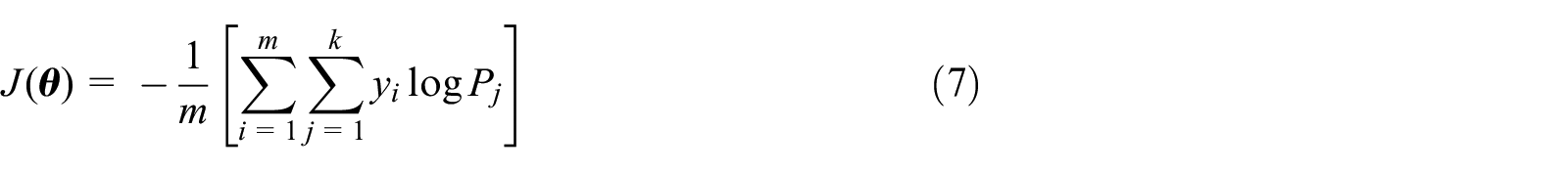
The fully-connected layers are the final layers of CNN. They are located behind the pooling layers, and each neuron is fully connected with all the neurons in the previous layers. The function of the fully-connected layer is to map the multi-dimensional features obtained from convolution and pooling operations to the sample space and complete the final classification. As the dimension of the input characteristic graph has been greatly reduced after several times of convolution and pooling operations, the fully-connected layers do not increase too much computation time. The sigmoid function is used for the two classification problems, and the Softmax function can be used for the k classification problems. The definition of the Softmax function is as follows

P_{j} = \frac{e^{θ_{y_{j}}^{T}}}{\sum_{l = 1}^{k} e^{θ_{yl}^{T}}}

(6)

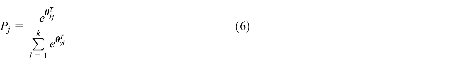
The corresponding loss function can be defined as

J (θ) = - \frac{1}{m} [\sum_{i = 1}^{m} \sum_{j = 1}^{k} y_{i} \log P_{j}]

(7)

where, $x_{i}$ is the vector of training data, m is the number of training data, $y_{i} \in {1, 2, \dots, k}$ is the category label of training data, k is the number of category label, θ is the parameter vector of the fully connection layer.

Network architecture

In this section, the network architecture and parameters of 1D-LeNet-5, 1D-AlexNet, and the proposed ODCNN are introduced in details.

1D-LeNet-5 architecture

The structure of 1D-LeNet-5 is shown in Figure 1. It consists of two convolutional layers, two average-pooling layers, followed by three fully-connected layers. The function of convolutional and average layers are extracting features of input signals, while the fully-connected layers are used to classify the extracted features.²⁶

Figure 1.

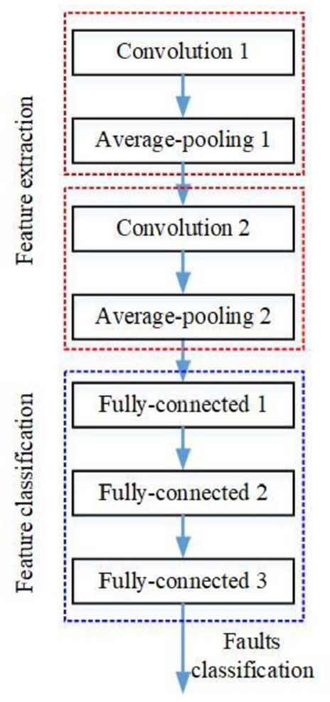
The architecture of 1D-LeNet-5.

The first layer of 1D-LeNet-5 is the input layer, which is a convolutional layer with filters having size 50 and a stride of 1. The next layer is an average-pooling layer (also called sub-sampling layer) with the kernel size 2 and stride of 1. The similar convolutional and average-pooling layers are followed in layers 3 and 4, and parameters of these two layers are same to the former two layers. The output of 1D-LeNet-5 consists of three fully-connected layers, the units of two former layers (layers 5 and 6) are 200, and all of these units in the sixth layer is connected to all nodes in the fifth layer. The last layer is a Softmax classifier with 10 units which is used to recognize the labels from 0 to 9. The detail structural parameters of 1D-LeNet-5 are given in Table 1.

Table 1.

Parameters of 1D-LeNet-5.

No. layers	Type of layer	No. neurons	Size of kernel	Strides
1	Convolution	10	50	1
2	Average-pooling	10	2	1
3	Convolution	20	50	1
4	Average-pooling	20	2	1
5	Fully-connected	200	–	–
6	Fully-connected	200	–	–
7	Fully-connected	10	–	–

1D-AlexNet architecture

The layers of 1D-AlexNet²⁷ are much larger and deeper than 1D-LeNet-5, which contains five convolutional layers, three max pooling layers and three fully connected layers.

The convolutional layer 1 (kernel size 50, stride 4) and 2 (kernel size 50, stride 1) connect the max-pooling layers with kernel size 3 and stride of 2. Convolutional layers 3, 4, and 5 are connected directly with kernel size 2 and a stride of 1. Then, the fifth convolutional layer is followed by a max-pooling layer with kernel size 3 and a stride of 2. The output of 1D-AlexNet consists of three fully-connected layers, the units of two former layers (layers 9 and 10) are 200, and all of these units in the 10th layer is connected to all nodes in the ninth layer. The last layer is a Softmax classifier with 10 units which is used to recognize the labels from 0 to 9. The structure of 1D-AlexNet is shown in Figure 2 and the detail structural parameters of 1D-AlexNet are listed in Table 2.

Figure 2.

The architecture of 1D-AlexNet.

Table 2.

Parameters of 1D-AlexNet.

No. layers	Type of layer	No. neurons	Size of kernel	Strides
1	Convolution	10	50	4
2	Max-pooling	10	3	2
3	Convolution	20	50	1
4	Max-pooling	20	3	2
5	Convolution	50	2	1
6	Convolution	50	2	1
7	Convolution	25	2	1
8	Max-pooling	25	3	2
9	Fully-connected	200	–	–
10	Fully-connected	200	–	–
11	Fully-connected	10	–	–

ODCNN architecture

The architecture of our presented ODCNN is illustrated in Figure 3, which is deeper than traditional CNNs. It consists of six groups of convolutional and max-pooling layers, followed by three fully-connected layers. In this network, the max-pooling layer is introduced repeatedly to enhance the classification capability and to improve the robustness of extracted features. Compared with the 1D-LeNet-5 and 1D-AlexNet Networks, the proposed ODCNN can increase the accuracy significantly.

Figure 3.

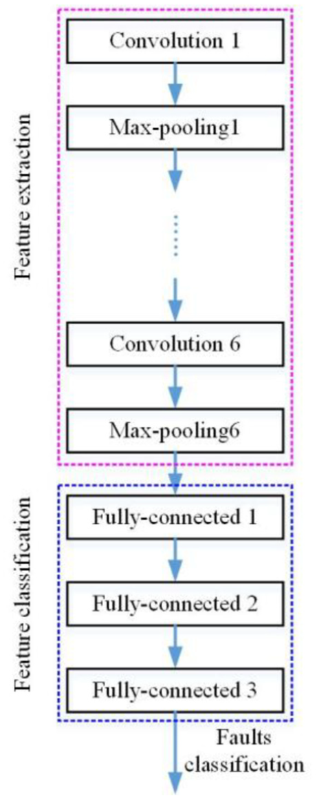
The architecture of ODCNN.

The first layer of ODCNN is the input layer, which is a convolutional layer with filters having size 50 and a stride of 4. A max-pooling layer with the kernel size 3 and stride of 2 is followed. The similar convolutional and max-pooling layers are followed in layers 3 and 4, parameters of layer 3 with the kernel size 50 and stride of 1, and parameters of layer 4 with the kernel size 3 and stride of 2. Then, two sets of convolutional and max-pooling layers are followed in layers 5 to 8, where parameters of layers 5 and 7 with the kernel size 5 and stride of 1, and parameters of layers 6 and 8 with the kernel size 3 and stride of 2. Subsequently, two groups of convolutional and max-pooling layers are followed in layers 9 to 12, where parameters of layers 9 and 11 with the kernel size 2 and stride of 1, and parameters of layers 10 and 12 with the kernel size 2 and stride of 2. The output of ODCNN also consists of three fully-connected layers, the units of two former layers (layers 13 and 14) are 200, and all of these units in the 14th layer is connected to all nodes in the 13th layer. The last layer is a Softmax classifier with 10 units which is used to recognize the labels from 0 to 9. In order to effectively suppress over-fitting phenomena and improve the capability of this network, the dropout algorithm is used in fully connected layers, and the parameters are set as 0.5. The corresponding structural parameters of ODCNN are given in Table 3.

Table 3.

Parameters of proposed ODCNN.

No. layers	Type of layer	No. neurons	Size of kernel	Strides
1	Convolution	20	50	4
2	Max-pooling	20	3	2
3	Convolution	50	50	1
4	Max-pooling	50	3	2
5	Convolution	60	5	1
6	Max-pooling	60	3	2
7	Convolution	60	5	1
8	Max-pooling	60	3	2
9	Convolution	50	2	1
10	Max-pooling	50	2	2
11	Convolution	20	2	1
12	Max-pooling	20	2	2
13	Fully-connected	200	–	–
14	Fully-connected	200	–	–
15	Fully-connected	10	–	–

Case study

In this section, the experimental apparatus used to obtain the rolling bearings vibration signals of normal and different fault types is depicted. In addition, the data processing technology is presented in detail.

Description of the experimental apparatus

In order to make a comparative study on the capability of three models, the vibration data provided in the Open Bearing Database of Case Western Reserve University (CWRU) are applied for analysis, the corresponding experimental platform is shown in Figure 4.²⁸

Figure 4.

Experimental apparatus.

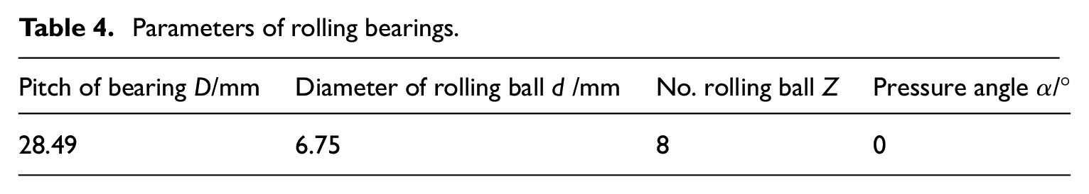
It consists of a torque transducer, a dynamometer and a power motor. The left-most motor is used to generate driving force, and the right-most dynamometer is used to generate rated loads (0hp, 1hp, 2hP and 3hp), which connected with a mediated torque sensor. The testing rolling bearings support the motor shaft and the basic parameters of the bearing used in the experiment is given in Table 4. Both of the drive and fan ends of the motor housing are attached the accelerometers with the magnetic bases in the vertical direction. Vibration signals are acquired under different working conditions including normal and faulty situations. The electrical discharge machining (EDM) method is applied on the test bearing in the diameters of 7, 14, and 21 mils (1 mil = 0.001 inches) to simulate different fault types of rolling bearings. The vibration signals were collected with the speed of 12kS/s, and the data of drive end bearing faults is collected with the speed of 48kS/s. The system simulates the normal state (NB) and three kinds of fault types, namely, inner ring (IR), rolling balls (RB), and outer ring (OR) faults, and each type of fault consists of three fault sizes (7, 14, and 21 inches, respectively). Therefore, there are 10 kinds of running states of bearings. The description of rolling bearings fault types is given in Table 5. The time-domain vibration signals of rolling bearing for normal state, inner ring, rolling balls, and outer ring faults are illustrated in Figure 5.

Table 4.

Parameters of rolling bearings.

Pitch of bearing D/mm	Diameter of rolling ball d /mm	No. rolling ball Z	Pressure angle α/°
28.49	6.75	8	0

Table 5.

The faults classification of rolling bearings.

Fault types	Length of dataset	Fault identification	Category labels
Normal	1024	NB	0
Fault of inner race (7 in)	1024	IR07	1
Fault of inner race (14 in)	1024	IR14	2
Fault of inner race (21 in)	1024	IR21	3
Fault of rolling balls (7 in)	1024	RE07	4
Fault of rolling balls (14 in)	1024	RE14	5
Fault of rolling balls (21 in)	1024	RE21	6
Fault of outer race (7 in)	1024	OR07	7
Fault of outer race (14 in)	1024	OR14	8
Fault of outer race (21 in)	1024	OR21	9

Figure 5.

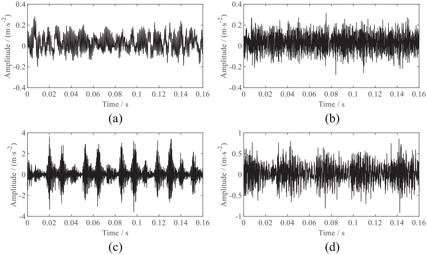
Time-domain vibration signals of rolling bearing. (a) Normal state. (b) Rolling balls. (c) Outer ring. (d) Inner ring.

Data augmentation

In order to realize high accuracy fault diagnosis, the number of training samples needs to be large enough. However, the sample size of CWRU Bearing Data center is limited. In this paper, the overlap method is applied to increase the number of training and testing samples. Figure 6 depicts the sketch map of this method, which slices the vibration signals of rolling bearings with overlap.²⁵

Figure 6.

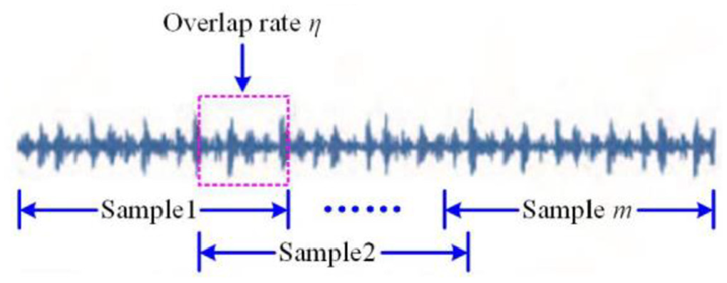
Data argumentation by overlapping.

With the method of overlap, the training and testing samples are obtained. x is the vibration signal of rolling bearings, and assuming the total length of it is N, the length of sample is n, the maximum number of segmented samples m can be obtained with overlap rate η is as follows

m = ⌊ \frac{N - n}{n \times η} ⌋

(8)

where ⌊•⌋ is round down operation.

The ith sample is

y_{i} = x [(i - 1) \times n \times η + 1, (i - 1) \times n \times η + n] i \in [1, m]

(9)

where x is the vibration signals of bearing; $y_{i}$ is the ith data sample after segment; the overlap rate η can be set as needed. In this paper, it is set as 0.4, that is, $η = 0.4$ .

Dataset A, B, C, and D represent load of 0, 1, 2, and 3hp, respectively. Dataset A contains 400 training samples and 180 testing samples, while for Dataset B, C, and D, each one contains 1000 training and 180 testing samples with 10 different fault types. The details of all the datasets are shown in Table 6.

Table 6.

Bearing datasets.

Dataset classification	Datasets
	Dataset A	Dataset B	Dataset C	Dataset D
Training	400	1000	1000	1000
Testing	180	180	180	180

Validation and analysis

In this section, the classification accuracy and convergence comparisons among the 1D-LeNet-5, 1D-AlexNet, and ODCNN models is carried out using the datasets obtained in Section 3. In addition, the feature visualization for the three CNNs is presented and discussed.

Analysis and discussion

Classification accuracy of different CNNs

Three experiments are implemented: the first two experiments are carried out to determine the training and testing accuracy of 1D-LeNet-5 and 1D-AlexNet using datasets disposed in Section 3.2 (refer to Table 6), while the diagnostic capability of the proposed ODCNN using the same datasets is implemented finally. The accuracy of classification is calculated as follows

A_{a} = \frac{\sum_{i = 1}^{m} A_{i}}{m} \times 100 %

(10)

where A_a is the average classification accuracy; A_i is the classification accuracy of four datasets (dataset A, B, C and D); m is the number of datasets, that is, m = 4.

The training and testing accuracy of three approaches are shown in Tables 7 –9. Compared with 1D-LeNet-5 and 1D-AlexNet, the ODCNN proposed in this paper possess better recognition capability. The recognition accuracy of four datasets from high to low are A, B, C, and D. It is presumed that the increase of load leads to the increase of vibration and noise of the system, which will reduce the bearing fault recognition rate.²⁹

Table 7.

Accuracy of 1D-LeNet-5.

Accuracy	Datasets
	Dataset A	Dataset B	Dataset C	Dataset D	A_a
Training accuracy (%)	100	100	100	100	100
Testing accuracy (%)	99.78	99.52	99.28	98.73	99.32

Table 8.

Accuracy of 1D-AlexNet.

Accuracy	Datasets
	Dataset A	Dataset B	Dataset C	Dataset D	A_a
Training accuracy (%)	99.68	98.93	99.37	98.20	99.05
Testing accuracy (%)	99.78	99.7	99.39	98.78	99.41

Table 9.

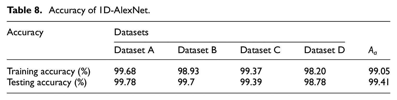
Accuracy of ODCNN.

Accuracy	Datasets
	Dataset A	Dataset B	Dataset C	Dataset D	A_a
Training accuracy (%)	99.19	99.58	99.79	99.33	99.47
Testing accuracy (%)	99.89	99.76	99.64	99.03	99.58

In order to clearly show the fault recognition ability of three CNNs, the confusion matrix is introduced to analyze the prediction results of three models in details. Figure 7 shows the confusion matrixes of three models in the load of 3hp. It can be found that in three models, the diagnostic accuracy of NB, IR07, IR21, RE14, RE21, and OR07 is high, while it is rather poor in the 14 inch of Outer race (OR14). Compared with 1D-LeNet-5 and 1D-AlexNet, the ODCNN increases the diagnostic rate in RE07 significantly.

Figure 7.

The confusion matrix of three CNNs. (a) 1D-LeNet-5. (b) 1D-AlexNet. (c) ONCNN.

Convergence analysis

Figure 8 illustrates the iterative process of training and validation accuracy with corresponding loss functions of these algorithms, which can examine the convergence speed of these algorithms. The training and validation accuracy curves in Figure 8 indicate that the three algorithms can reach high accuracy. The training and validation loss curves show that the three algorithms have good convergence performance.

Figure 8.

The accuracy and loss function of three different CNNs. (a) 1D-LeNet-5. (b) 1D-AlexNet. (c) ODCNN.

Feature visualization

To demonstrate the effective and feature extraction capability of the presented ODCNN, the t-distributed stochastic neighbor embedding (t-SNE) technique is applied to reduce the dimension of the extracted features for visualization. This method is an efficient nonlinear dimensionality reduction approach that can transform the data in high dimensional space into a lower one for visualization.

Taking the dataset D for example, the two-dimensional visualizations of fault features in three CNNs, which are extracted from the Softmax classifier, are depicted in Figure 9, in which different colors represent different fault types of rolling bearings. In addition, it is noteworthy that the visualization of three CNNs reveals some interesting phenomena. Firstly, the feature discrimination of three CNNs gradually becomes obvious. As shown in Figure 9(a), it is not divisible in 1D-LeNet-5. While in ODCNN, the discrimination of fault features is more significant as shown in Figure 9(c) because layers of three CNNs are deeper and wider. Secondly, Figure 9(a) and (b) reveal that the visualization of RE07 and OR14 have some overlapped regions, indicating that the fault types of RE07 and OR14 may not easy to be discriminated. However, the proposed ODCNN can solve the problems effectively as shown in Figure 9(c).

Figure 9.

Feature visualization of three CNNs. (a) 1D-LeNet-5. (b) 1D-AlexNet. (c) ODCNN.

Conclusions

To realize high-precision and intelligent fault diagnosis of rolling bearings, a novel CNN with one-dimensional structure is proposed in this paper. Compared with 1D-LeNet-5 and 1D-AlexNet CNN, the proposed approach is deeper and wider. The feature extraction is realized by six sets of convolutional and max pooling layers, which has a better performance to extract as more features of the rolling bearing vibration signals as possible. The experimental results indicate that the proposed ODCNN possess good classification capacity and sufficient accuracy. The visualization of the feature distribution via t-SNE method indicates that it has better classification performance than traditional CNNs.

Although the proposed approach has above advantages, there is still room for improvement in our future work. In fact, the data filter is very necessary before the feature classification, for the raw bearing vibration data quality significantly affects the accuracy and convergence of classification in practical application. Remarkably, the proposed ODCNN is expected to be widely used in the fault diagnosis of other similar types of one-dimensional time signals, like voice recognition, atrial fibrillation, and rotating machinery vibration.

Footnotes

Declaration of conflicting interests

The author(s) declared no potential conflicts of interest with respect to the research, authorship, and/or publication of this article.

Funding

The author(s) disclosed receipt of the followin g financial support for the research, authorship, and/or publication of this article: This work is supported by Natural Science Foundation of Zhejiang Province of China under Grant LQ20E050017, National Key Technologies Research & Development Program of China under Grant 2018YFF0212702, Zhejiang Lab’s International Talent Fund for Young Professionals under Grant ZJ2019JS006 and National Natural Science Foundation of China under Grant 61801454.

ORCID iD

Shenglong Xie

Author biographies

Shenglong Xie was born in Anqing, China, in 1988. He received the B.S. degree in mechanical design, manufacturing and automation and the M.S. degree in mechatronic engineering from Anhui University of Technology, Ma’anshan, China, in 2011 and 2014, respectively. He received his Ph.D. degree in mechanical engineering from Tianjin University, Tianjin, China, in 2018. He was a Visiting Researcher with the National Institute of Metrology, Beijing, China (from March 2019 to Jan 2020). He is a Postdoctoral at Faculty of Mechanical Engineering and Automation, Zhejiang Sci-Tech University, Hangzhou, China. Currently he is Lecturer at School of Mechanical and Electrical Engineering, China Jiliang University, Hangzhou, China. His research interests include motion control of rehabilitation and industrial robots, modeling and control of pneumatic muscle actuators with hysteresis.

Guoying Ren was born in Kaifeng, China, in 1979. He received the B.S. degree in Mechanical Engineering and Automation from the China University of Mining and Technology, Xuzhou, China, in 2002, and the M.S. degree in metrological technology and instruments from the National Institute of Metrology, Beijing, China, in 2005. He is currently pursuing the Ph.D. degree from the Tianjin University. His research interests include Length metrology, robot measurement technology and material thermal property metrology.

Junjiang Zhu received the M.S. and Ph.D. degrees in Mechanical Engineering from Huazhong university of Science and Technology, Wuhan, China, in 2011 and 2015, respectively. He is currently an Assistant Professor in School of Mechatronic Engineering, China Jiliang university, Hangzhou, China. His current research interests include signal processing and deep learning.

References

Udmale

Singh

SK.

Application of spectral kurtosis and improved extreme learning machine for bearing fault classification. IEEE Trans Instrum Meas 2019; 68(11): 4222–4233.

Zhou

Cheng

YJ.

Fault diagnosis for rolling bearing under variable conditions based on image recognition. Shock Vib 2016; 1–14.

You

Fan

, et al. A fault diagnosis model for rotating machinery using VWC and MSFLA-SVM based on vibration signal analysis. Shock Vib 2019; 1–16.

Wang

Hou

Tang

, et al. Fault detection enhancement in rolling element bearings via peak-based multiscale decomposition and envelope demodulation. Math Probl Eng 2014; 1–12.

Liu

Zhou

, et al. A statistical feature investigation of the spalling propagation assessment for a ball bearing. Mech Mach Theory 2019; 131: 336–350.

Sopon

, et al. Fault features extraction for bearing prognostics. J Intell Manuf 2012; 23(2): 313–321.

Zhang

Liu

Chen

, et al. Fault diagnosis of rotating machinery based on kernel density estimation and Kullback-Leibler divergence. J Mech Sci Technol 2014; 28(11): 4441–4454.

Huang

Zhang

Approximate entropy as a nonlinear feature parameter for fault diagnosis in rotating machinery. Meas Sci Technol 2012; 23(4): 45603–45616.

Liu

Rolling bearing fault diagnosis based on STFT-Deep learning and sound signals. Shock Vib 2016; 1–12.

10.

Kumar

Srinivasa

Vijay

, et al. Wavelet transform for bearing condition monitoring and fault diagnosis: a review. Int J Comadem 2014; 17(1): 9–23.

11.

Lei

Lin

, et al. Fault diagnosis of rotating machinery based on an adaptive ensemble empirical mode decomposition. Sensors 2013; 13(12): 16950–16964.

12.

Tian

, et al. Rolling bearing fault diagnosis under variable conditions using LMD-SVD and extreme learning machine. Mech Mach Theory 2015; 90: 175–186.

13.

Widodo

Son

Yang

, et al. Fault diagnosis of low speed bearing based on relevance vector machine and support vector machine. Expert Syst Appl 2009; 36(3): 7252–7261.

14.

Wang

Tang

, et al. A compound fault diagnosis for rolling bearings method based on blind source separation and ensemble empirical mode decomposition. PloS One 2014; 9(10): e109166.

15.

Chen

Randall

RB.

Intelligent diagnosis of bearing knock faults in internal combustion engines using vibration simulation. Mech Mach Theory 2016; 104: 161–176.

16.

Moosavian

Ahmadi

Tabatabaeefar

, et al. Comparison of two classifiers: K-nearest neighbor and artificial neural network, for fault diagnosis on a main engine journal-bearing. Shock Vib 2013; 20: 263–272.

17.

Jalali

Ghandi

Motamedi

Intelligent condition monitoring of ball bearings faults by combination of genetic algorithm and support vector machines. J Nondestr Eval 2020; 39(1).

18.

Sanchez

Zurita

, et al. Multimodal deep support vector classification with homologous features and its application to gearbox fault diagnosis. Neurocomputing 2015; 168: 119–127.

19.

Yuan

Adaptive fault diagnosis algorithm for rolling bearings based on one-dimensional convolutional neural network. Chinese J Sci Inst 2018; 39(7): 134–143.

20.

Wen

Gao

, et al. A new convolutional neural network based data-driven fault diagnosis method. IEEE Trans Ind Electron 2017; 99(1): 1–9.

21.

Hoang

Kang

HJ.

Rolling element bearing fault diagnosis using convolutional neural network and vibration image. Cogn Syst Res 2019; 53: 42–50.

22.

Jian

Guo

, et al. Fault diagnosis of motor bearings based on a one-dimensional fusion neural network. Sensors 2019; 19(122): 1–16.

23.

Janssens

Slavkovikj

Vervisch

, et al. Convolutional neural network based fault detection for rotating machinery. J Sound Vib 2016; 377: 331–345.

24.

Sadoughi

Physics-based convolutional neural network for fault diagnosis of rolling element bearings. IEEE Sens 2019; 19(11): 4181–4192.

25.

Zhang

Peng

, et al. A deep convolutional neural network with new training methods for bearing fault diagnosis under noisy environment and different working load. Mech Syst Signal Process 2018; 100: 439–453.

26.

Rashad

AJ.

Handwriting Arabic character recognition LeNet using neural network. Int Arab J Inf Techn 2009; 6(3): 304–309.

27.

Alex

Ilya

Geoffrey

EH.

Imagenet classification with deep convolutional neural networks. Communications of the ACM 2017; 60(6): 84–90.

28.

Jian

Qing

Liang

, et al. Fault diagnosis of motor bearing based on deep learning. Adv Mech Eng 2019; 11(9): 1–9.

29.

Zhou

Sun

Cao

Vibration and noise characteristics of a gear reducer under different operation conditions. J Low Freq Noise V A 2019; 1–18.

Application of a new one-dimensional deep convolutional neural network for intelligent fault diagnosis of rolling bearings

Abstract

Keywords

Introduction

Theory of CNN

Convolutional layer

Pooling layer

Fully-connected layer

Network architecture

1D-LeNet-5 architecture

1D-AlexNet architecture

ODCNN architecture

Case study

Description of the experimental apparatus

Data augmentation

Validation and analysis

Analysis and discussion

Classification accuracy of different CNNs

Convergence analysis

Feature visualization

Conclusions

Footnotes

Declaration of conflicting interests

Funding

ORCID iD

Author biographies

References