Convolutional neural network with Huffman pooling for handling data with insufficient categories: A novel method for anomaly detection and fault diagnosis

Abstract

The rotating component is an important part of the modern mechanical equipment, and its health status has a great impact on whether the equipment can safely operate. In recent years, convolutional neural network has been widely used to identify the health status of the rotor system. Previous studies are mostly based on the premise that training set and testing set have the same categories. However, because the actual operating conditions of mechanical equipment are complex and changeable, the real diagnostic tasks usually have greater diversity than the pre-acquired datasets. The inconsistency of the categories of training set and testing set makes it easy for convolutional neural network to identify the unknown fault data as normal data, which is very fatal to equipment health management. To overcome the above problem, this article proposes a new method, Huffman-convolutional neural network, to improve the generalization ability of the model in detection task with various operating conditions. First, a new Huffman pooling kernel is designed according to the Huffman coding principle and the Huffman pooling layer structure is introduced in the convolutional neural network to enhance the model's ability to extract common features of data under different conditions. Second, a new objective function is proposed based on softmax loss, intra-class loss, and inter-class loss to improve the Huffman-convolutional neural network's ability to distinguish different classes of data and aggregate the same class of data. Third, the proposed method is tested on three different datasets to verify the generalization ability of the Huffman-convolutional neural network in diagnosis tasks with multi-operating conditions. Compared with other traditional methods, the proposed method has better performance and greater potential in multi-condition fault diagnosis and anomaly detection tasks with inconsistent class spaces.

Introduction

The continuous development of modern industrial technology has prompted more and more large-scale, complicated, integrated, and intelligent equipment to emerge. The above characteristics of modern industrial equipment not only makes higher operational reliability, safety, and economy become urgent needs, but also create new challenges for equipment condition monitoring and maintenance management.^1–3 The fault diagnosis and anomaly detection technology developed under this background performs a vital function in ensuring the safe and sustainable operation of modern mechanical systems.

Fault diagnosis or anomaly detection is essentially a pattern recognition process that establishes a mapping of the measurement or feature space to the fault space. Generally, fault diagnosis methods can be divided into four categories: model-based method, signal-based method, knowledge-based method, and hybrid method.^4–6

Traditional identification processes typically rely on a variety of ancillary maps of the monitoring signals and are ultimately diagnosed by a diagnostician. For example, the spectrum of the vibration signal, the envelope spectrum, and the demodulation spectrum are applied to diagnose the failure of the rotating machinery.^7–11

Knowledge-based method is a very typical automatic fault identification method that requires a large amount of historic data to establish the system fault modes without prior known models or signal patterns. With the advent of the era of big data, knowledge-based fault diagnosis methods have been flourishing.^12,13 The data-driven fault diagnosis method represented by machine learning (ML) and deep learning (DL) is especially typical. The vibration signals are projected into a nonlinear space by methods such as locally linear embedding, ¹⁴ sparse representation, ¹⁵ autoencoder, ¹⁶ and support vector machines (SVMs) ¹⁷ to obtain more significant features. Deep belief network (DBN), ¹⁸ convolutional neural network (CNN), ¹⁹ sparse autoencoder, ²⁰ stacked denoising autoencoder, ²¹ sparse filtering, ²² and other DL methods can improve the accuracy of recognition without manual feature extraction.

The fault diagnosis methods based on ML and DL introduced above are all based on a common assumption that the class labels of the test data and training data are consistent.^23,24 However, in the actual fault diagnosis task, different working conditions and even new fault types will lead to inconsistency between the test data and the training data category. ²⁵ With the in-depth study of intelligent diagnosis technology, in the field of rotating equipment fault diagnosis, researchers’ attention on the diagnosis problem has gradually shifted from the consistent category space to the inconsistent category space. The category space inconsistency in the fault diagnosis problem mainly includes equipment inconsistency, working condition inconsistency, and fault class inconsistency. From this, techniques such as open-set fault diagnosis (OSFD) ²⁶ and cross-domain fault diagnosis (CDFD) ²⁷ are derived.

The OSFD is mainly used to solve fault diagnosis problems in which there are more fault classes in test data than in training data. This requires the diagnostic model to not only correctly classify known categories but also to identify new categories that have not been seen before. Therefore, the common solution of OSFD is to first build a feature extraction model, then design a feature measurement method such as a distance-based method, and further set a reasonable threshold to evaluate whether the tested data belongs to a known class. Tian et al. proposed a feature fusion method based on t-sne and kernel null Foley–Sammon transform (KNFST) to construct the state feature space of the equipment, and then designed an adaptive threshold based on the test data to improve the accuracy of classifying known faults and identifying unknown faults. ²⁸ Lundgren and Jung employed a probability density function (PDF) to abstract the failure characteristics of the data and proposed a one-class classifier using the approximate distinguishability measure to test if a new PDF p can be explained by a known fault mode $f_j$ . ²⁹ To achieve OSFD, they used a one-class classifier for each fault mode $f_j$ and designed a tuning strategy for the threshold $K_j$ of each classifier to achieve the classification of known faults and the identification of unknown faults.

Different from OSFD, CDFD focuses on solving fault diagnosis problems across working conditions or across equipment. The main idea of solving CDFD is domain adaptation (DA),^30,31 which is a technique of transfer learning. ³² The core idea of DA is to reduce the distribution discrepancy between the source domain (SD) and the target domain (TD) to achieve the purpose of classifying the TD only by training the SD data or a small amount of TD data. Therefore, how to represent the features of the SD and the TD, how to measure the distribution difference between the SD and the TD, and how to reduce the distribution discrepancy between the SD and the TD have become the hot research directions of DA. Qin et al. adopted modified composite multi-scale fuzzy entropy (MCMFEs) as the fault features to express similar features information between the TD and the SD. ³³ Further, they proposed a feature similarity measurement method based on minimum redundancy maximum relevance (mRMR), Kullback–Liebler divergence (KLD), and k-nearest neighbor (KNN) to improve the classification accuracy of CDFD for rolling bearing. Li et al. present a knowledge mapping-based adversarial domain adaptation (KMADA) method to learn a distance metric measured by a discriminator. ³⁴ This method requires the construction of 2D feature images of each domain via short-time Fourier transform (STFT) and L2 normalization.

Both OSFD and CDFD are very complex in various stages of organizing data, building diagnostic models, and training diagnostic models. Because the models are too complex, the computational loss is also very large. Considering that in actual engineering, the occurring possibility of faults in the initial stage of equipment operation is relatively small. Before a device fails or new faults occur, we can often collect some valid data of the device. At the same time, for the equipment that fails, we usually shut down the equipment directly, and the technicians will conduct a detailed inspection to determine the specific fault mode and formulate maintenance strategies. Therefore, for an automatic diagnosis model, it is more engineering meaningful to be able to identify a new fault as an anomaly than to identify that the fault is a new fault.

In view of the abovementioned fault diagnosis engineering requirements, this article attempts to improve the generalization ability of simple networks, so that it can solve the problems of fault diagnosis and anomaly detection under the condition of multiple operating conditions and inconsistent class labels. This article mainly studies fault diagnosis and anomaly detection tasks under the condition that the category of testing data is larger than training data. It is found that Huffman coding can effectively reduce the noise of the vibration signal of the rotor equipment and enhance the impact characteristics of the vibration signal in our previous study. ³⁵ Considering that some effective feature information will be lost in the preprocessing of vibration signal, we try to combine Huffman coding with CNN, and conduct Huffman coding on the data stream during the CNN feature extraction process. In view of CNN's weak ability to identify unknown test samples, we further enhanced CNN's ability to describe normal data by increasing the distribution difference between classes of known training data to isolate the characteristic space of normal data. For this reason, we introduce mixed loss into the new network objective function. With the help of the Huffman coding and mixed loss, the network could improve the accuracy on classifying the testing data which has more diversity than the training data.

The main contributions of the proposed method are as follows:

We propose a new pooling method called Huffman pooling according to the principle of Huffman coding and introduce it into the traditional CNN. Compared with traditional pooling methods such as max pooling and average pooling, the Huffman pooling method can not only preserve the numerical information within each pooling unit but also the complexity information within the pooling unit. The Huffman pooling process effectively retains more information related to the original data features so it can effectively enhance the robustness of the CNN model.

We design a new H-CNN objective function based on softmax loss, intra-class loss, and inter-class loss. Compared with the traditional loss function, the new loss function can not only guide the model to learn the features of the same class of samples, but also guide the model to distinguish the features of different classes of samples so it can effectively improve the generalization ability of the model for fault diagnosis and anomaly detection under multiple operating conditions.

To verify the generalization ability of the H-CNN in fault diagnosis and anomaly detection under multiple working conditions, the proposed method is tested on three different datasets which are the cylindrical roller bearings dataset, deep groove ball bearings dataset, and gearbox dataset. In the detection tasks for known faults and unknown faults, the accuracy rate reaches 95.37/91.93, 98.62/95.27, and 99.79/96.32 respectively. Compared with other methods, the H-CNN has higher accuracy.

The rest of this article is organized as follows. The basic theory of Huffman average code length (HACL) and the CNNs is presented in Basic theory section. Proposed method for fault diagnosis section elaborates on the pooling method based on Huffman coding theory, the structure of the fault diagnosis model based on Huffman pooling and CNN, and a new mixed loss function. In Case studies section, the identification performance of the proposed method is verified on three datasets. Finally, the concluding remarks are summarized in Conclusion section.

Basic theory

HACL

Huffman coding is a method of optimal prefix coding used for lossless data compression. Since David A. Huffman proposed the coding algorithm in 1952, ³⁶ Huffman coding has been widely used in the field of computer science and information theory due to its high efficiency. The output of Huffman's algorithm is essentially a variable-length code table with which source symbols can be binary encoded. The algorithm derives the code table from the frequency of occurrence of all possible values of the source symbol.

Let the symbol set $A=\{a_1,a_2,\cdots ,a_n\}$ , and the corresponding probability is $P=\{p_1,p_2,\cdots ,p_n\}$ , $p_i=probability(a_i)$ , $1\le i\le n$ . The Huffman code of A is $C(P)=\{c_1,c_2,\cdots ,c_n\}$ , where $c_i$ is the codeword for $a_i$ , $1\le i\le n$ . The HACL of A can be solved as follows:

Step 1: Let $A^{*}=A$ , $P^{*}=P$ , $A^{*}$ and $P^{*}$ will change in the coding process. The size of $A^{*}$ and $P^{*}$ is n at the beginning of the encoding.

Step 2: Let $A^{\mathrm{\prime }}$ be the set obtained by rearranging $A^{*}$ in descending order of probability $P^{*}$ . $A^{\mathrm{\prime }}=\{a_1^{\mathrm{\prime }},a_2^{\mathrm{\prime }},\cdots ,a_{m-1}^{\mathrm{\prime }},a_m^{\mathrm{\prime }}\}$ , $m$ is the size of $A$ .

Step 3: Take the two symbols $a_{m-1}^{\mathrm{\prime }}$ and $a_m^{\mathrm{\prime }}$ with the least probability in the symbols sequence. Encode the symbol $a_{m-1}^{\mathrm{\prime }}$ with higher probability into “1” and the symbol $a_m^{\mathrm{\prime }}$ with less probability as “0”. Add the probabilities ( $p_{m-1}^{\mathrm{\prime }}$ and $p_m^{\mathrm{\prime }}$ ) of the two symbols as the probability $p^{*}$ of the new symbol $a^{*}$ . Delete $a_{m-1}^{\mathrm{\prime }}$ and $a_m^{\mathrm{\prime }}$ from $A^{\mathrm{\prime }}$ . Add $a^{*}$ into $A^{\mathrm{\prime }}$ . Then the set $A^{\mathrm{\prime }}$ has changed into ${A^{\mathrm{\prime }}}^{\mathrm{\prime }}$ and the size of ${A^{\mathrm{\prime }}}^{\mathrm{\prime }}$ is $m-1$ . Let $A^{*}={A^{\mathrm{\prime }}}^{\mathrm{\prime }}$ .

Step 4: Repeat Step 2 and Step 3 until there is only one symbol in set $A^{*}$ and the probability of $a^{*}$ is 1.

Step 5: Backtrack from the symbol with the probability of 1 to each source symbol and record 0/1 in the backtracking path. The Huffman code of $a_i$ is $c_i$ .

Step 6: The HACL of each source symbol $a_i$ is calculated according to the length of $c_i$ and the corresponding probability $p_i$ as follows:

$$HACL={\left(\sum p_i\right)}^{-1}\sum _{i=1}^n{p}_i^{*}length(c_i)$$

(1)

For a set of source symbols $U=\{u_1,u_2,u_3,u_4,u_5,u_6\}$ with probabilities $P=\{p_1,p_2,p_3,p_4,p_5,p_6\}$ , $p_1=0.45$ , $p_2=0.16$ , $p_3=0.13$ , $p_4=0.12$ , $p_5=0.09$ , and $p_6=0.05$ , the process of Huffman coding is presented in Figure 1.

Figure 1.

The process of Huffman coding.

Let the code length of the ith symbol in U is $l_i$ . It can be seen from Figure 1 that $l_1=1$ , $l_2=3$ , $l_3=3$ , $l_4=3$ , $l_5=4$ , and $l_6=4$ . The HACL of the probability sequence is calculated as $HACL=p_1*l_1+p_2*l_2+p_3*l_3+p_4*l_4+p_5*l_5+p_6*l_6=2.24$ .

CNNs

CNN is generally composed of three parts: input layer, hidden layer, and output layer. The input layer is the original data such as images. The output layer is the result of classifying the features. The hidden layers are neuron layers with complex multilayer nonlinear structure, including convolution layers, activate layers, subsampling layers, and perceptron layers. A convolution layer, an activate layer, and a subsampling layer are combined into a feature extraction unit. The perceptron layers classify features by mapping them to class labels. The classification ability of the CNN model can be improved by optimizing the feature extraction layers and the perceptron layers. The structure of the CNN is shown in Figure 2.

Figure 2.

The structure of a convolutional neural network (CNN).

Figure 2 shows a simple CNN with two convolutional layers (C1, C2), two activate layers, and two subsampling layers (S1 and S2) in the feature extraction layer. After multiple feature extractions, the single-layer perceptron transforms the final 2D feature map into 1D matrix. The output layer divides the features into N classes. The single-layer perceptron is usually a fully connected structure.

Convolutional layer

Convolutional layers are the core component of hidden layers. A convolutional layer is composed of multiple stacked convolution kernels. The convolution kernel is like a filter, which can extract features at a smaller scale on the data input to the convolutional layer. The information of the input data is enhanced, and the interference of noise is suppressed. The size of the convolution kernel is called the receptive field. The input and output of a convolutional layer are both feature maps. The value of the output feature map can be calculated by equation (2).

$${\mathbf{z}}_k={\mathbf{w}}_k\otimes \mathbf{x}+b_k$$

(2)

where ${\mathbf{w}}_k$ is the weight vector of the kth convolution kernel, $\mathbf{x}$ is the input feature map, $b_k$ is the bias of the kth convolutional kernel, ${\mathbf{z}}_k$ is the output feature map, and $\otimes$ is convolution operation. For example, there is an input feature map $\mathbf{x}$ with a size of $4\times 4$ , a convolution kernel ${\mathbf{w}}_k$ with a size of $2\times 2$ , and the sliding step parameter $stride$ of the convolution kernel is 1. The process of the convolution operation by kth convolution kernel can be expressed as shown in Figure 3.

Figure 3.

Process of convolution operation.

Activate layer

CNN simulates the response of human brain nerves to different stimuli using nonlinear activation layers. The introduction of nonlinear activation layers enables CNNs to handle complex computational problems. Commonly used activation functions include sigmoid function, Tanh function, and ReLU function. The formulas of these functions are as follows:

$$Sigmoid(x)=1/(1+e^x)$$

(3)

$$Tanh(x)=(e^x-e^{-x})/(e^x+e^{-x})$$

(4)

$$ReLU(x)=max(0,x)$$

(5)

Subsampling layer

The subsampling layer reduces the amount of computation and abstracts the features by downsampling the output feature map of the convolution layer. Subsampling layers are also known as pooling layers. Commonly used pooling methods are max pooling and average pooling. For example, the size of a feature map processed by an activation layer is $4\times 4$ , the pooling size is $2\times 2$ , and the sliding step parameter $stride$ is 2. The common pooling process is shown in Figure 4.

Figure 4.

Process of max pooling and average pooling operation.

Perceptron layer

The perception layer is usually a fully connected structure. The fully connected layers are the last few layers in the CNN and act as the classifier. Another main role of the perception layer connected to the hidden layer is to convert the 2D feature map into a 1D feature matrix. Each node of the fully connected layer is fully interconnected with the nodes of the previous layer. The fully connected layer performs weighted summation of the features output by the previous layer and inputs the result to the output layer. The formula of the fully connected layer is as follows:

$${\mathbf{z}}_i={\sum }_{i=1}^n{w}_i{x}_i+b_i$$

(6)

where $w_i$ is the weight coefficient of the fully connected layer, $x_i$ is the value of the ith neuron in the previous layer, and $b_i$ is the bias of the fully connected layer.

Output layer

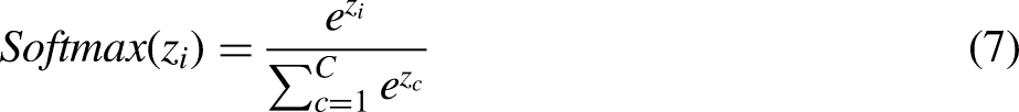
For classification issues, the softmax function is usually applied in the output layer. The formula of the softmax function is as follows:

$$Softmax(z_i)={\displaystyle \frac{e^{z_i}}{{\sum }_{c=1}^C{e}^{z_c}}}$$

(7)

Proposed method for fault diagnosis

CNN updates the weights of the network by the back-propagation algorithm based on the loss between the predicted label and the true label. The network could obtain a high identification accuracy once the loss function is converged to a global minimum value. Considering that the working conditions of rotating equipment in engineering practice are complex and changeable, this section proposes a new loss function and a new network structure to improve the generalization ability of CNN.

Generally, the objective function of CNN is defined to minimize the loss between the predicted table and the real table. When the loss function converges to the global minimum, CNN has a high recognition accuracy. Considering the complex and changeable working conditions of rotating equipment in engineering practice, the data categories to be detected are far more than the available data categories, so CNN cannot learn all the labels to be tested. Therefore, a new loss function and a new network structure are proposed in this section to improve the generalization ability of CNN and try to solve the problem of fault diagnosis and anomaly detection under the condition of insufficient categories of training data.

Signal to 2D image conversion method

Since most of the traditional data-driven methods for diagnosis cannot directly process the original data, many researchers design different data preprocessing methods to improve the feature expression ability of the original data. However, the characteristics obtained by different treatment methods are also different, so it has a great influence on the result. Wen et al. proposed an effective data preprocessing method to maximize the retention of the original data. ²⁵ The idea of this method is to convert the time-domain signal into an image by fulfilling the pixels calculated by the value of the signal. For a signal $L(n)$ , the image can be obtained as follows.

Step 1: Select a segment $L^{\mathrm{\prime }}(M^2)$ with length $M^2$ randomly from $L(n)$ , $M^2\le n$ , $L^{\mathrm{\prime }}(M^2)=\{L_1^{\mathrm{\prime }},L_2^{\mathrm{\prime }},\cdots ,L_{M^2}^{\mathrm{\prime }}\}$

Step 2: Generate a blank image of size $M\times M$ .

Step 3: Let $M(i,j)$ be the pixel strength of the image, $i=1,2,\cdots ,M$ , $j=1,2,\cdots ,M$ . The pixels of the image can be fulfilled by equation (8), where round $(*)$ is the rounding function.

$$M(i,j)=round\left\{{\displaystyle \frac{{L^{\mathrm{\prime }}}_{((i-1{)}^{*}M+j)}-Min(L^{\mathrm{\prime }})}{Max(L^{\mathrm{\prime }})-Min(L^{\mathrm{\prime }})}\times 255}\right\}$$

(8)

Figure 5 shows the image converted from raw signals.

Figure 5.

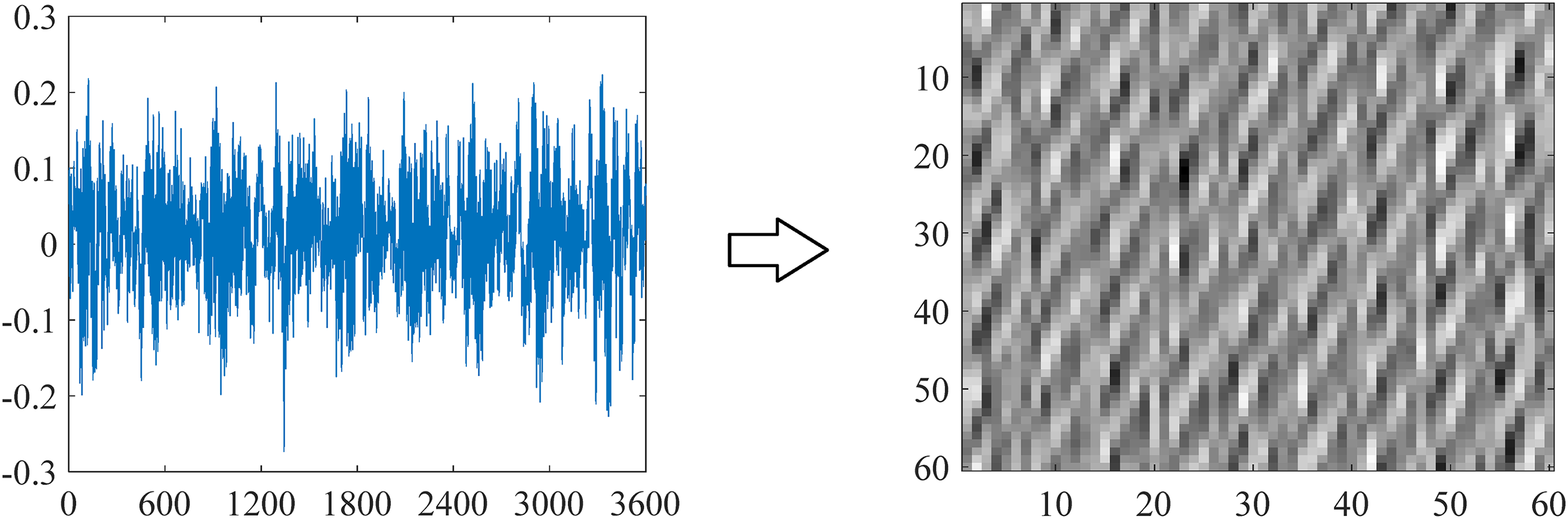
Signal to 2D image conversion.

Huffman pooling

It can be seen from the above Huffman coding process that if Huffman coding is performed on a time series, the amount of data can be effectively reduced, and the dimensionality reduction effect can be achieved.

To analyze the influence of Huffman coding on the data better, this article takes the famous dataset of bearing vibration signal of the famous Case Western Reserve University as an example. Since the vibration signal is a series of vibration amplitudes in the time domain, the data itself usually contains negative values. According to the method of solving the HACL, the signal needs to be converted into a discrete point sequence with probability meaning. Therefore, the original signal needs to be processed into a nonnegative sequence first and then converted into a probability sequence. As shown in Figure 6, the probability sequence is transformed into HACLs finally.

Figure 6.

Probability sequence-to-HACLs conversion method.

For a signal data $X(n)=\{x_1,x_2,\cdots ,x_n\}$ , the HACL sequence is obtained as follows:

Step 1: According to equation (9), convert signal amplitude to nonnegative value $X^{\mathrm{\prime }}(n)=\{x_1^{\mathrm{\prime }},x_2^{\mathrm{\prime }},\cdots ,x_n^{\mathrm{\prime }}\}$ .

$$x_i^{\mathrm{\prime }}=x_i-min[X(n)],i=1,2,\cdots ,n$$

(9)

Step 2: According to equation (10), transform $X^{\mathrm{\prime }}(n)=\{x_1^{\mathrm{\prime }},x_2^{\mathrm{\prime }},\cdots ,x_n^{\mathrm{\prime }}\}$ to probability sequence $P(n)=\{p_1,p_2,\cdots ,p_n\}$ .

$$p_i=x_i^{\mathrm{\prime }}/{\sum }_{j=1}^n{x^{\mathrm{\prime }}}_j$$

(10)

Step 3: Divide $P(n)=\{p_1,p_2,\cdots ,p_n\}$ into different segments $G(m)=\{g_1,g_2,\cdots ,g_m\}$ with the sliding window, where $g_i=\{p_{i+s*(i-1)},p_{i+s*(i-1)+1},\cdots ,p_{i+s*(i-1)+l-1}\}$ , l is the length of the window, s is the step size of sliding window movement. The size of $G(m)$ can be solved according to equation (11), where $floor(*)$ means finding the biggest integer smaller than ${}^{*}$ .

$$m=floor\left({\displaystyle \frac{n-l}{s}}\right)+1$$

(11)

Step 4: Calculate the HACL sequence as

$$HACLs=\{HACL(g_1),HACL(g_2),\cdots ,HACL(g_m)\}.$$

This article applies the HACLs method to the SKF 6205-2rs bearing test data of Western Reserve University. ³⁷ The vibration signal was collected under 0hp load condition, and the corresponding speed was 1797 r/min. There are four types of data in this dataset, including normal (N), inner race fault (IF), outer race fault (OF), and ball fault (BF). Each type of fault contains three damage sizes (0.178 mm, 0.356 mm, and 0.533 mm). The HACLs for the above 10 different types of vibration signals are calculated by setting $l=5,8,11,16,20,25$ and $s=1,4,7,10$ .

To better illustrate the influence of HACLs on the signal, this article analyzes from three perspectives of time domain, frequency domain, and distribution in 2D feature space.

The waveforms of the raw signals and their HACLs with $(l,s)=(5,1)$ are shown in Figure 7. It can be seen that the HACLs can weaken the common vibration component in the original signal to a certain extent in the time domain. The impact component of the signal is enhanced at the same time.

Figure 7.

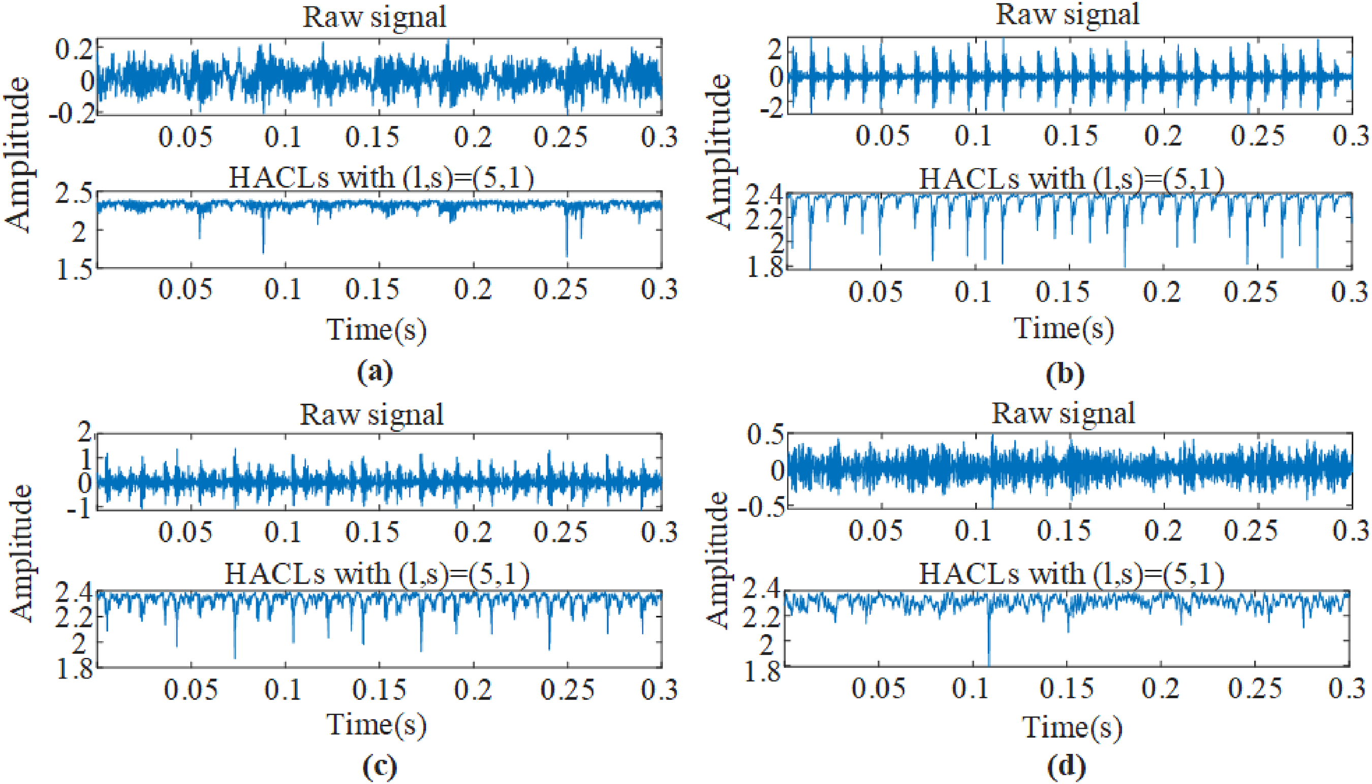
The waveforms of raw signals and their HACLs with $(l,s)=(5,1)$ . (a) Normal (N), (b) outer race fault (OF), (c) inner race fault (IF), and (d) ball fault (BF).

Combined with the relevant parameters used in the bearing experiment, it can be calculated that the rotating frequency is 29.95Hz under the 0hp load condition. The characteristic frequencies corresponding to IF, OF, and BF are 162.19Hz, 107.36Hz, and 141.17Hz respectively. For the raw signals as shown in Figure 7, the amplitude spectrum and envelope spectrum were analyzed respectively. For the HACLs, only the amplitude spectrum was analyzed. The results are presented in Figure 8.

Figure 8.

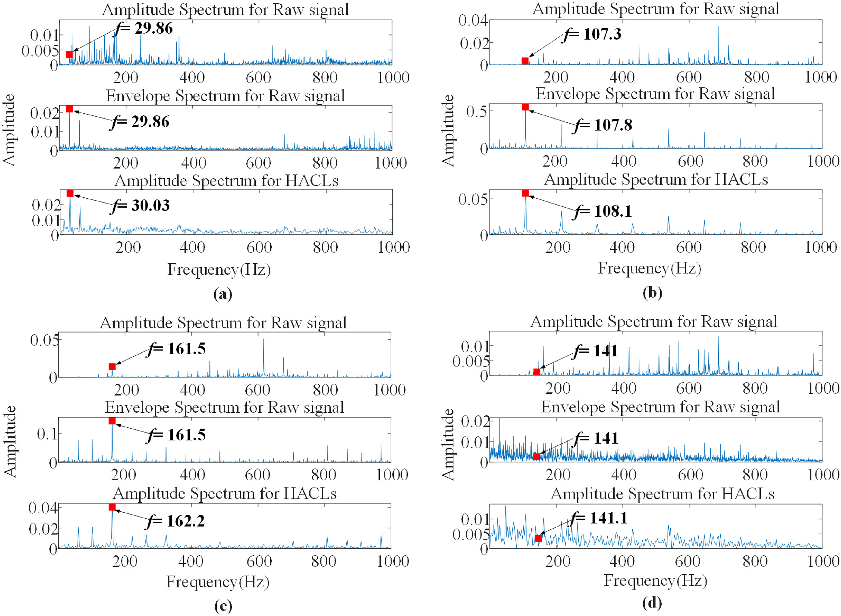
The frequency analysis results of raw signals and their HACLs. (a) Normal (N), (b) outer race fault (OF), (c) inner race fault (IF), and (d) ball fault (BF).

It can be seen from Figure 8 that it is difficult to obtain the characteristic frequency of the original signal in the low-frequency band by directly analyzing the amplitude spectrum. When Fourier spectrum analysis of the original signal is performed directly, the fault frequency will exist in the sideband of the high frequency, which makes it difficult to intuitively find the fault frequency in the low-frequency band. However, by calculating the envelope spectrum of the original signal, it can be found that the characteristic frequency can be observed very intuitively in the low-frequency band. By comparing the envelope spectrum for raw signals and amplitude spectrum for HACLs, it is not difficult to find that for HACLs, only amplitude spectrum analysis is needed to get the obvious fault characteristic frequency in the low-frequency band. It indicates that HACLs has a similar effect to the envelope spectrum.

To better illustrate the influence of HACLs on the distribution in 2D feature space, the t-sne method was applied to visualize the original data and their HACLs with different parameters. ³⁸ The feature distribution in 2D space is presented in Figure 9.

Figure 9.

The feature distribution of raw signal and HACLs in 2D space. (a) Raw signal and (b) HACLs with different parameters. The “-1”, “-2”, and “-3” in the legend means the damage size of the fault is 0.178 mm, 0.356 mm, 0.533 mm respectively.

It is obvious that the data of the same type and degree of failure in the original data are not concentrated in the feature space, but HACLs with appropriate parameters in the feature space show more concentration of the same type of data, and low concentration of different types of data. In addition, the distribution of HACLs in the feature space also has the following characteristics:

When the parameters are selected properly, HACLs can increase the degree of dispersion between normal data and abnormal data, which has guiding significance for quickly determining whether the rotor equipment is abnormal in engineering practice;

No matter what parameters are selected, the distribution area of the rolling element failure samples is always close to the areas of the other three types of samples, which is consistent with the propagation mechanism of rolling element failures. Due to the particularity of the rolling element structure, when it fails, it will indirectly cause the abnormal vibration of the inner ring, the outer ring, and the entire experimental equipment by means of vibration transmission, and as the effect of the fault continues to spread, the failure energy of the rolling element itself will gradually decrease, so whether in the time-frequency domain analysis or in the characteristic distribution analysis, the fault characteristics of the rolling element itself are easily covered by the fault characteristics of the inner and outer rings;

It can be seen from Figure 9 that when l is const and s has less influence on the distribution of HACLs in the feature space. But when s is constant and l changes from small to large, the concentration of HACLs of the same data varies greatly. For example, when $l=11,20,25$ , the degree of concentration is high, but when $l=8,16$ , the degree of concentration is low.

From the above analysis of the distribution of HACLs in the time domain, frequency domain, and feature space, the following conclusions can be drawn: HACLs can effectively enhance the impact components in the original signal, remove high-frequency components, and keep the fault characteristic frequency unchanged. At the same time, HACLs can enhance the degree of aggregation of the same type of original data in the feature space and provide convenience for further analysis of the health status and fault type of the equipment. However, different calculation parameters have a greater impact on the distribution characteristics of the data in the feature space.

In view of the characteristics of the abovementioned HACLs, this article proposes a method of fusing HACLs and CNN. By applying HACLs to the pooling operation of CNN, it can not only reduce the dimensionality in the pooling process, but also retain more features of the original signal.

According to the above introduction to the Huffman coding method, the process of solving HACL fully considers the impact of all data. Therefore, this method can be applied to the pooling process of the CNN.

CNN is a network connected layer by layer with three different functions: convolutional layer; pooling layer; fully connected layer. The convolutional layer applies multiple filters to obtain the feature map of the input image. The pooling layer abstracts the features by reducing the input feature dimension by means of downsampling. The features are extracted by alternating convolutional layer and pooling layer. The abstract features are finally input to the full connection layer to calculate the classification results

Set the output size of the ith convolutional layer is $N*M$ , the ith Huffman pooling kernel size is $n*m$ . The sliding steps of the pooling kernel along the rows and columns are $ste{p}_n$ and $ste{p}_m$ respectively. These parameters need to satisfy the following constraints: (i) N-n is divisible by $ste{p}_n$ and (ii) M-m is divisible by $ste{p}_m$ . Figure 10 shows how the Huffman pooling layer works.

Figure 10.

The ith Huffman pooling layer.

According to the method of calculating HACL, the data needs to be converted into a discrete point sequence with probability meaning. Therefore, the output data of ith convolutional layer needs to be processed into a nonnegative data first and then converted into a probability sequence. As shown in Figure 10, the output of ith convolutional layer is normalized before pooling.

For a 2D data $X(N,M)=\{x_{11},x_{12},\cdots ,x_{1M};\begin{array}{c}\end{array}{x}_{21},x_{22},\cdots ,x_{2M};\begin{array}{c}\end{array}\cdots ;\begin{array}{c}\end{array}{x}_{N1},x_{N2},\cdots ,x_{NM}\}$ , the HACL 2D data is obtained as follows:

Step 1: According to equation (12), transform the signal amplitude to nonnegative value $X^{\mathrm{\prime }}(N,M)=\{x_{11}^{\mathrm{\prime }},x_{12}^{\mathrm{\prime }},\cdots ,x_{1M}^{\mathrm{\prime }};\begin{array}{c}\end{array}{x}_{21}^{\mathrm{\prime }},x_{22}^{\mathrm{\prime }},\cdots ,x_{2M}^{\mathrm{\prime }};\begin{array}{c}\end{array}\cdots ;\begin{array}{c}\end{array}{x}_{N1}^{\mathrm{\prime }},x_{N2}^{\mathrm{\prime }},\cdots ,x_{NM}^{\mathrm{\prime }}\}$ .

$$x_{ij}^{\mathrm{\prime }}=x_{ij}-min[X(N,M)]\begin{array}{c},\end{array}i=1,2,\cdots ,N;j=1,2,\cdots ,M$$

(12)

Step 2: According to equation (13), transform $X^{\mathrm{\prime }}(N,M)$ to $P(N,M)$ , $P(N,M)=\{p_{11},p_{12},\cdots ,p_{1M};\begin{array}{c}\end{array}{p}_{21},p_{22},\cdots ,p_{2M};\begin{array}{c}\end{array}\cdots ;\begin{array}{c}\end{array}{p}_{N1},p_{N2},\cdots ,p_{NM}\},p_{ij}\in [0,1]$ .

$$p_{ij}=x_{ij}^{\mathrm{\prime }}/{\sum }_{i=1,j=1}^N{x^{\mathrm{\prime }}}_{ij}$$

(13)

Step 3: Divide $P(N,M)$ into different blocks according to the sliding window with step size $ste{p}_n$ and $ste{p}_m$ .

Step 4: Calculate each block as $HACL$ into $G(N^{\mathrm{\prime }},M^{\mathrm{\prime }})$ . The size of $G(N^{\mathrm{\prime }},M^{\mathrm{\prime }})$ can be calculated according to equation (14).

$$N^{\mathrm{\prime }}={\displaystyle \frac{N-n}{ste{p}_n},M^{\mathrm{\prime }}={\displaystyle \frac{M-m}{ste{p}_m}}}$$

(14)

This article compares the differences between Huffman pooling and the traditional pooling methods with three sets of examples. The three sets and the results of different methods are listed in Table 1. Obviously, when the data length and shape change, the results calculated by the max pooling and average pooling methods may be the same, but the results calculated by the Huffman pooling method are significantly different. Therefore, the Huffman pooling method can effectively reduce the data dimension while retaining the differences between different data.

Table 1.

The results of different pooling methods.

Data	Max pooling	Average pooling	Huffman pooling
[0.1 0.2 0.3 0.4]	0.4	0.25	1.9
[0.1 0.1 0.4 0.4]	0.4	0.25	1.8
[0.05 0.3 0.4]	0.4	0.25	1.4667

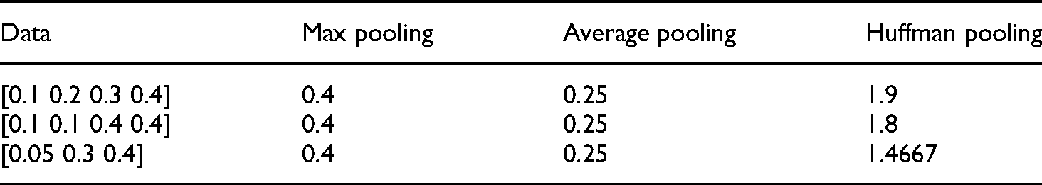
It can be seen from Table 1 that for three different sets of data, the results of max pooling and average pooling methods are the same, which cannot reflect the difference of the original data, but the results of Huffman pooling on different data are obviously different. Therefore, the Huffman pooling presented in this article can not only achieve dimensionality reduction sampling, but also retain the different characteristics between the original data.

Huffman-CNN (H-CNN) construction

The ability of CNN to extract and classify features of research objects has been widely verified in the field of image recognition. For signals that have been converted to images, a CNN can train them and classify them well.

This article proposes the H-CNN based on the Huffman pooling and CNN mentioned above. The network structure includes a feature extraction stage and a classification stage. The feature extraction contains convolution layers, batch normalization layers, ReLU activation layers, and pooling layers. The classification stage is realized by the full connection layer.

The structures of the typical CNN and H-CNN for $60\times 60$ images are shown in Figure 11. In these two structures， we set $N=M$ and $ste{p}_n=ste{p}_m=n=m$ . The parameters on each layer are presented in Table 2. The denotation of Conv $(5\times 5\times 32)$ means that it is a convolutional layer where the filter size is $5\times 5$ with 32 channels. Maxpool $(2\times 2)$ means that it is a maxpool layer with $(2\times 2)$ filers. Huffman pool $(2\times 2)$ means that it is a Huffman pooling layer with $(2\times 2)$ filers.

Figure 11.

The structure of the neural networks: (a) A typical convolutional neural network (CNN) structure for $60\times 60$ images and (b) a Huffman-convolutional neural network (H-CNN) structure for $60\times 60$ images.

Table 2.

Layer configurations of CNN and H-CNN models.

Layer name	CNN models	H-CNN models	Activation
L1	Conv $(5\times 5\times 32)$	Conv $(5\times 5\times 32)$	ReLU
L2	Maxpool $(2\times 2)$	Huffman pool $(2\times 2)$	-
L3	Conv $(5\times 5\times 64)$	Conv $(5\times 5\times 64)$	ReLU
L4	Maxpool $(2\times 2)$	Huffman pool $(2\times 2)$	-
L5	Conv $(3\times 3\times 128)$	Conv $(3\times 3\times 128)$	ReLU
L6	Maxpool $(2\times 2)$	Huffman pool $(2\times 2)$	-
Classification	-	-	Softmax

CNN: convolutional neural network; H-CNN: Huffman-convolutional neural network.

The new mixed loss function

Minimizing the distance between the distribution of training set and testing set is a common method to reduce generalization error on test set. When there are unknown faults in the diagnosis task, it is very difficult to predict the distribution of test set directly because no prior information about fault mode and fault degree can be obtained. To solve the above problems, a feasible solution is to make full use of the training set and establish the feature boundary between normal samples and fault samples by CNN. Although the feature boundary cannot be directly used to diagnose unknown fault types, it can be used to determine whether unknown data is abnormal. Therefore, a new mixing loss function is designed to improve the ability of the diagnostic model in homogeneous aggregation and heterogeneous differentiation. This is also an attempt to construct the feature boundary.

Generally, the loss function of CNN is designed according to the difference between the output of the network and the real label. As the training set of $\{(X_i,y_i){\}}_{i=1}^n$ , $X_i$ is the input data, $y_i$ is the corresponding label, n is the number of classes. The corresponding output of CNN is $y_i^{\mathrm{\prime }}$ . The traditional loss function can be represented as follows:

$$L=\sum _{i=1}^n|{y^{\mathrm{\prime }}}_i-y_i|$$

(15)

In practice, a softmax classifier is usually used to classify the output of CNN, so the loss function is usually designed as follows: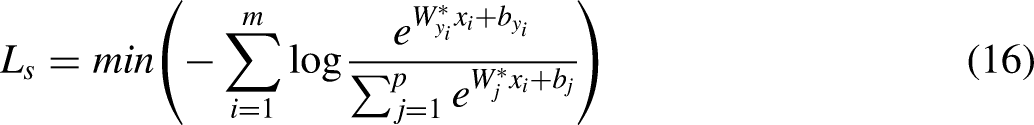

$$L_s=min\left(-\sum _{i=1}^m\log {\displaystyle \frac{e^{W_{y_i}^{*}{x}_i+b_{y_i}}}{{\sum }_{j=1}^p{e}^{W_j^{*}{x}_i+b_j}}}\right)$$

(16)

where m is the size of mini batch. $x_i$ is the i-th feature belonging to the $y_i$ . $W_j$ and $b_j$ is the j-th column of the weight and bias of the last fully connected layer, respectively.

In this article, we introduce a mixture loss function considering homogenous clustering and heterogeneous differentiation in traditional CNN. By minimizing intra-class variation and maximizing inter-class variation, the new loss can distinguish the characteristics of normal data and fault data. Under the guidance of mixed loss and softmax loss, the network can explore some commonalities of feature spaces under different working conditions. By learning the characteristics of known health data, the ability to identify unknown data as abnormal data can be improved. In this way, the network has good generalization performance for unknown health data.

The mixed loss function is proposed with reference to the idea of center loss. In the DL method for face recognition, ³⁹ the center loss is designed to enhance its recognition ability. The main idea behind center loss is to simultaneously learn the center of each class feature and penalize the distance between the feature and the corresponding class center.

In order to minimize the feature distance of intra-class and maximize the feature distance of inter-class, this article proposes a mixed loss function based on the distance between center point and feature. For the given set 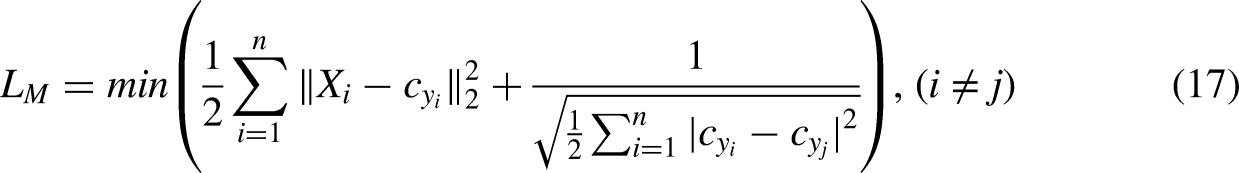$\{(X_i,y_i){\}}_{i=1}^n$ . The mixed loss is designed as follows:

$$L_M=min\left({\displaystyle \frac{1}{2}\sum _{i=1}^n\Vert X_i-c_{y_i}{\Vert }_2^2+{\displaystyle \frac{1}{\sqrt{\frac{1}{2}{\sum }_{i=1}^n{|c_{y_i}-c_{y_j}|}^2}}}}\right),(i\ne j)$$

(17)

where $c_{y_i}$ is the center point of features of class $y_i$ . In theory, $c_{y_i}$ should be computed considering the entire training samples. However, the training process of CNN relies on the minimum batch of samples. The center point can be updated by replacing the entire training set with small batches. In each iteration, the update of $c_{y_i}$ can be processed as equations (18) to (19). In this article, the scalar parameter $\alpha$ is set as the default value 0.5.

$$\mathrm{\Delta }{c}_{y_i}={\displaystyle \frac{\sum _{i=1}^n\delta (y_i=k{)}^{*}(c_k-X_i)}{1+\sum _{i=1}^n\delta (y_i=k)},\delta =\{\begin{array}{cc}1& y_i=k\\ 0& y_i\ne k\end{array}}$$

(18)

$$c_{y_i}^{t+1}=c_{y_i}^t+\alpha \mathrm{\Delta }{c}_{y_i}^t$$

(19)

To ensure the features of clustering and dispersion between classes, a new mixed loss is added based on softmax loss. Finally, the new CNN is trained by optimization algorithm to minimize the loss function. The final loss function of H-CNN is defined as follows:

$$L_{H-CNN}=L_s+\mu L_M$$

(20)

where $\mu$ is a scalar parameter, we set $\mu =1e^{-6}$ considering the order of magnitude difference between $L_s$ and $L_M$ .

Case studies

This article focuses on the bearings and gears which are most widely used as rotor components in mechanical equipment for fault diagnosis and abnormal detection based on vibration signal drive.

In this section, the proposed method H-CNN is conducted on three different datasets, which are the cylindrical roller bearings dataset, deep groove ball bearings dataset, and gearbox dataset. The comparison test is mainly for the H-CNN and some other methods.

Data acquisition

Many types of faults and failure modes can occur to bearings and gears in various rotating machinery systems. Vibration signals collected from such a system are usually used to reveal its health condition. There are three datasets to verify the proposed method, including two bearing datasets and a gearbox dataset.

In two bearing datasets, experimental data were collected on a test rig with symmetrical structure and replaceable bearings as shown in Figure 12. The experimental device is mainly composed of a driving motor, a loading system, a shaft, a conveyer belt, and two bearings. The fault parts are prepared by means of electro-discharge machining. The bearing data used in this article are all vibration signals in the vertical direction.

Figure 12.

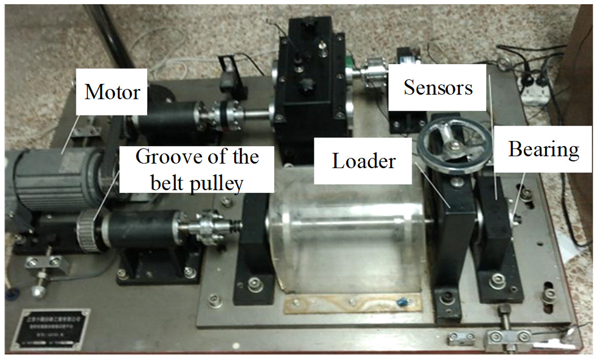
The bearing experimental rig.

In the gearbox dataset, the time-domain fault vibration data of gear is downloaded from the FigShare website. Cao et al. completed the experiment. ⁴⁰ The vibration signals are collected from a two-stage gearbox that is driven by a motor and loaded through a magnetic brake as shown in Figure 13. The torque is provided by a magnetic brake, which can be adjusted by changing the input voltage. A 32-tooth pinion and an 80-tooth pinion are mounted on the first stage input shaft. The second stage consists of a 48-tooth pinion and a 64-tooth pinion. The speed of the gears is controlled by an electric motor. Input shaft speed is measured by tachometer and gear vibration signals are collected by an accelerometer.

Figure 13.

The gearbox experimental rig.

Case 1: Cylindrical roller bearing

In the first bearing dataset, the test bearing is N205, a cylindrical roller bearing. The sampling frequency is 20 KHz. Seven health conditions are set as: normal; inner race with wear fault; outer race with breakage fault; roller with pitting fault; roller with groove fault; roller with wear failure; roller with missing piece fault. Figure 14 shows the fault bearings. Cylindrical roller bearings were tested under 15 load conditions, with the speed ranging from 100 r/min to 1500 r/min. For each health condition under a single load condition, the vibration signals were processed into a series of samples with a length of 3600.

Figure 14.

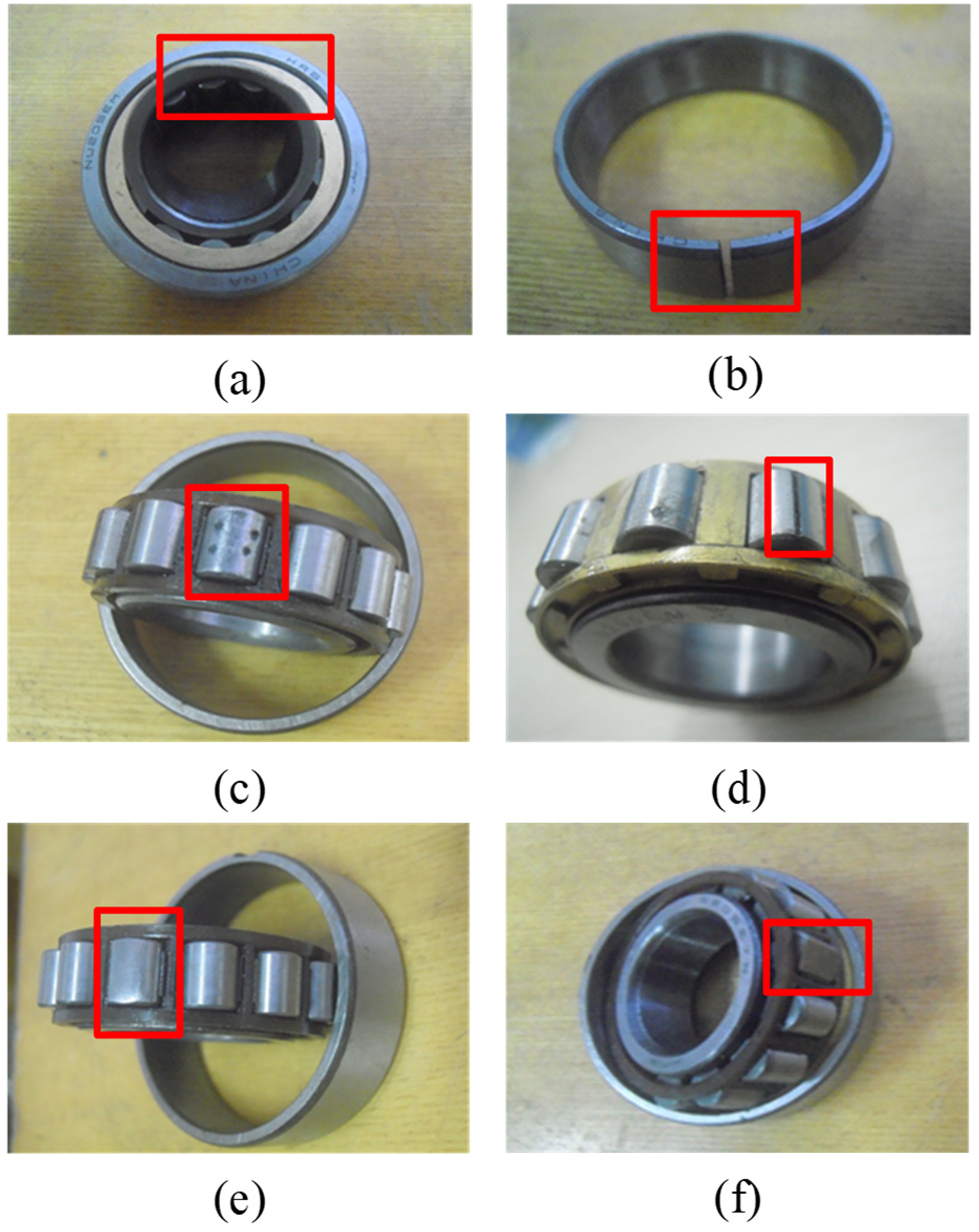
Six fault conditions of cylindrical roller bearings: (a) Inner race with wear fault, (b) outer race with breakage fault, (c) roller with pitting fault, (d) roller with groove fault, (e) roller with wear failure, and (f) roller with missing piece fault.

The samples are divided into training set and testing set. In order to prove that the method proposed in this article can identify whether the data of unknown health state is normal or not, we only use the normal data and four fault data, as shown in Figure 14(a) to (d) to train the network. The description of the cylindrical roller bearing data samples is listed in Table 3.

Table 3.

Label description of the cylindrical roller bearing dataset.

Class label	Load speed (×100r/min)	Health condition	Training set	Testing set
1	1/2/3/4/5/6/7/8/9/10/11/12/13/14/15	Normal	15 × 200	15 × 200
2	1/2/3/4/5/6/7/8/9/10/11/12/13/14/15	Inner race with wear fault	15 × 200	15 × 200
3	1/2/3/4/5/6/7/8/9/10/11/12/13/14/15	Outer race with breakage fault	15 × 200	15 × 200
4	1/2/3/4/5/6/7/8/9/10/11/12/13/14/15	Roller with pitting fault	15 × 200	15 × 200
5	1/2/3/4/5/6/7/8/9/10/11/12/13/14/15	Roller with groove fault	15 × 200	15 × 200
6	1/2/3/4/5/6/7/8/9/10/11/12/13/14/15	Roller with wear failure	–	15 × 200
7	1/2/3/4/5/6/7/8/9/10/11/12/13/14/15	Roller with missing piece fault	–	15 × 200

Case 2: Deep groove ball bearing

In the second bearing dataset, the test bearing is 6312, a deep groove ball bearing. The sampling frequency is 10 KHz. There are four load conditions, and the corresponding speeds range from 300 r/min to 1500 r/min (300/700/1100/1500). Five health conditions are set as normal; inner race with breakage fault; outer race with breakage fault; retainer with breakage fault; and ball with wear failure. The fault bearings are shown in Figure 15. For each health condition under a single load condition, the vibration signals were processed into a series of samples with a length of 3600.

Figure 15.

Four fault conditions of deep groove ball bearings: (a) Inner race with breakage fault, (b) outer race with breakage fault, (c) retainer with breakage fault, and (d) ball with wear failure.

The samples are also divided into training set and testing set. We use the normal data and three fault data, as shown in Figure 15(a) to (c) to train the network. A detailed description of the samples is listed in Table 4.

Case 3: Gearbox system

In the gearbox dataset, the sampling frequency is 20 KHz. The nine different conditions are introduced to the pinion on the input shaft: normal; missing tooth; root crack; spalling; and chipping tip with five different levels of severity (“chip5a”, “chip4a”, “chip3a”, “chip2a”, and “chip1a”). Figure 16 shows the different health conditions. For each health condition, the vibration signals are sliced into a series of samples with a length of 3600.

Figure 16.

Nine pinions with different health conditions.

Table 4.

Label description of the deep groove ball bearing dataset.

Class label	Load speed(r/min)	Health condition	Training set	Testing set
1	300/700/1100/1500	Normal	640	160
2	300/700/1100/1500	Inner race with breakage fault	640	160
3	300/700/1100/1500	Outer race with breakage fault	640	160
4	300/700/1100/1500	Retainer with breakage fault	640	160
5	300/700/1100/1500	Ball with wear failure	–	160

The samples are divided into training set and testing set. We use the normal data and six fault data (missing tooth/root crack/spalling/chip5a/ chip4a/chip3a) to train the network. A detailed description of the samples is listed in Table 5.

Table 5.

Label description of the gear dataset.

Class label	Health condition	Training set	Testing set
1	Normal	70	35
2	Missing tooth	70	35
3	Root crack	70	35
4	Spalling	70	35
5	Chip5a	70	35
6	Chip4a	70	35
7	Chip3a	70	35
8	Chip2a	–	35
9	Chip1a	–	35

Comparison methods

To evaluate the performance of the proposed H-CNN model, traditional CNN and some other methods are used in this article to compare the prediction accuracy of the three cases.

The traditional CNN methods used for comparison in this article include CNN-2D and CNN-1D. CNN-2D uses the same input data as H-CNN. Compared to H-CNN, CNN-2D only differs in the pooling layer. The structure of CNN-2D is shown in Figure 11(a) and Table 2. The input of CNN-1D is a 1D raw signal that has not been converted into 2D image. Meanwhile, the handcrafted features are extracted in time domain and frequency domain. The time domain is characterized by peak, peak to peak, absolute mean, standard variance, margin index, peak index, impulse factor, skewness index, and kurtosis index. In the frequency domain, there are six features, which are frequency center, root mean square frequency, SD frequency, and CP1, CP2, and CP3.^41,42 These statistical features are applied to shallow methods to classify health status. In this article, random forest (RF), SVM, KNN, and artificial neural network (ANN) are selected. In addition, some other advanced DL methods, including DBN, LSTM, and ResNet, are also used to compare and verify the effectiveness of the proposed method.

The average results of 10 tests are used as the evaluation basis in this article to reduce the error caused by randomness.

Results and discussion

Case 1: Cylindrical roller bearing

The images ( $60\times 60$ ) converted from cylindrical roller bearing raw signals are shown in Figure 17. It can be observed that the images under different operating conditions and different health conditions are totally different.

Figure 17.

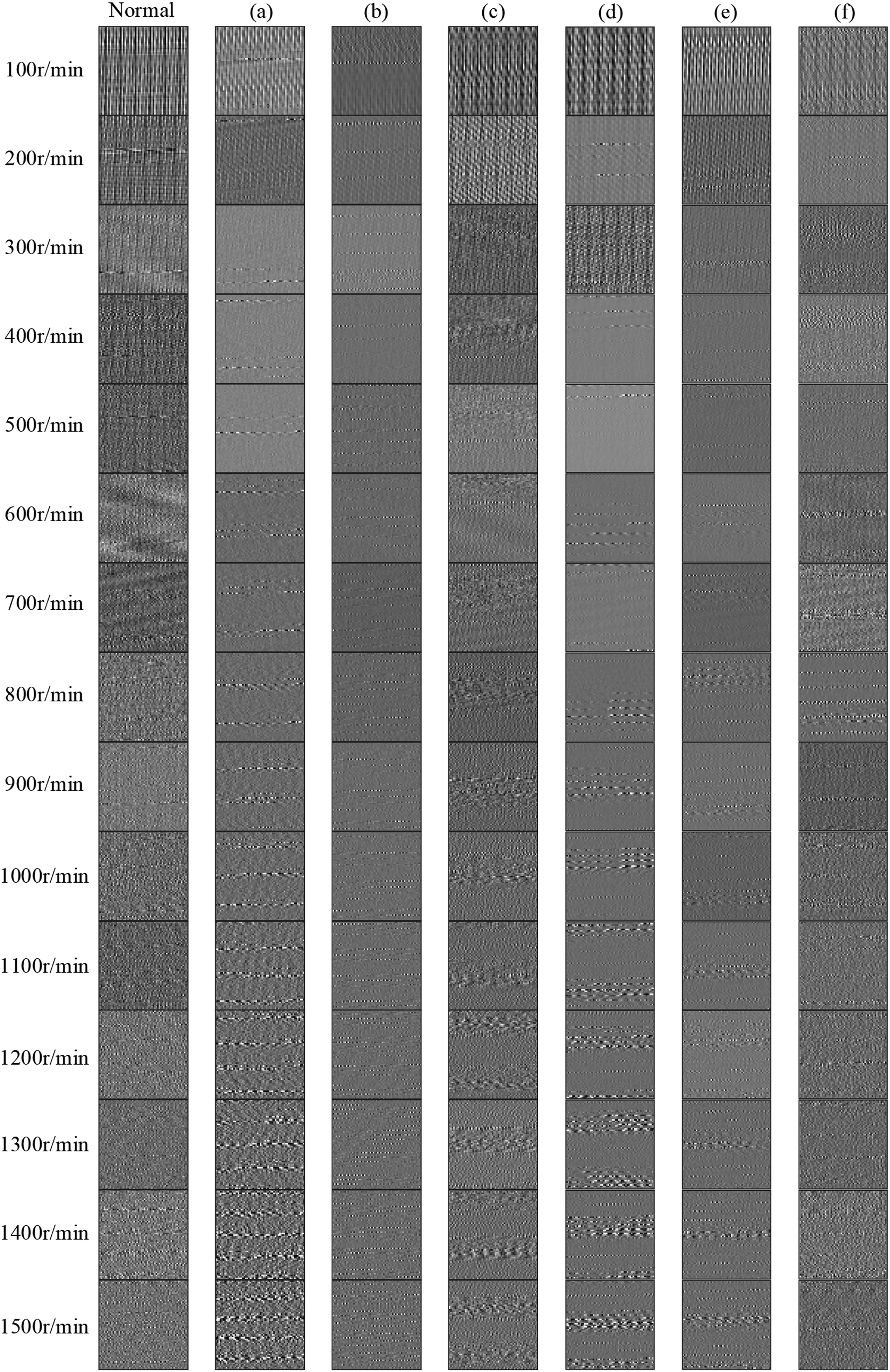
N205 cylindrical roller bearing raw signals conversion results: (a) Inner race with wear fault, (b) outer race with breakage fault, (c) roller with pitting fault, (d) roller with groove fault, (e) roller with wear failure, and (f) roller with missing piece fault.

Figure 18.

The confusion matrices of different methods in case 1: (a) SVM, (b) CNN, and (c) H-CNN.

As shown in Table 3, the training data contains five classes of data and the testing data contains seven classes of data in case 1. The accuracy of the recognition, in this case, is defined as follows:

$$\mathrm{Accuracy}=\{\begin{array}{cc}{\displaystyle \frac{N_{predict}(Labe{l}_{predict}=Labe{l}_{real})}{N_{label1-5}}}& Label:1-5\\ {\displaystyle \frac{N_{predict}(Labe{l}_{predict}\ne 1)}{N_{label6-7}}}& Label:6-7\end{array}$$

(21)

where $Labe{l}_{predict}$ is the output of the test data, $Labe{l}_{real}$ is the real label, and $N_{predict}(Labe{l}_{predict}=Labe{l}_{real})$ is the number of output labels is the same as the number of real labels. For the fault test data shown in Figure 17(e) and (f), as long as the network recognizes that the data is not normal, we assume that the prediction is correct.

The results of case 1 are shown in Table 6. It is obvious that the proposed H-CNN method obtains a better result compared with other methods in this case. The average prediction accuracy is as high as 95.37% for known data and 91.93% for unknown data. It is obvious that the proposed H-CNN performs better to deal with the unknown data. Although the traditional CNN-2D achieves higher accuracy for the known data, it is weak in identifying the classes which do not exist in the training data.

Table 6.

Comparison result of Huffman-convolutional neural network (H-CNN) and other methods in case 1 (%).

Methods	Average accuracy
	Known/Unknown
H-CNN	95.37/91.93
CNN-2D	97.79/88.66
CNN-1D	92.54/78.32
DBN	88.36/73.24
LSTM	91.62/65.57
ResNet	92.85/74.25
RF	81.64/71.46
KNN	72.39/65.83
SVM	77.63/70.34
ANN	68.43/59.63

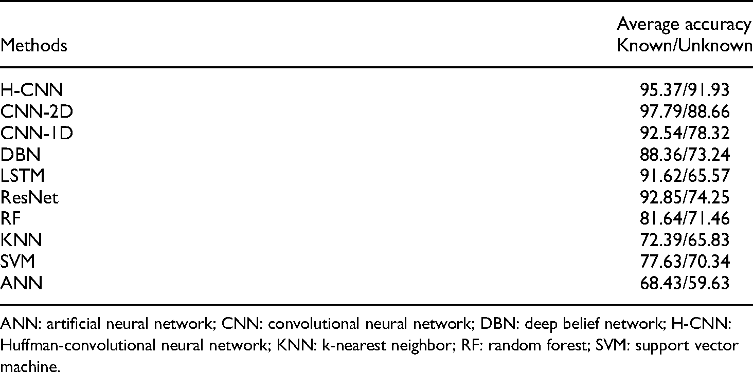
ANN: artificial neural network; CNN: convolutional neural network; DBN: deep belief network; H-CNN: Huffman-convolutional neural network; KNN: k-nearest neighbor; RF: random forest; SVM: support vector machine.

The confusion matrices of different methods in case 1 are shown in Figure18. SVM, CNN, and H-CNN mistake the data of fault (roller with wear failure) as normal data probability is 35.74%, 13.37%, and 9.65%, respectively. As for the fault (roller with missing piece fault), the misjudgment rates are 23.58%, 9.31%, and 6.49%, respectively. It is obvious that the traditional methods have poor ability to distinguish class labels 6–7. One of the possible reasons is that the proposed loss function can effectively enhance the difference between normal and abnormal data extracted by the network. So, the H-CNN has a better ability to identify fault data when the diversity of testing set is more than the training set.

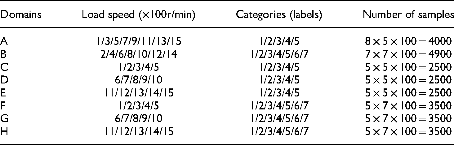
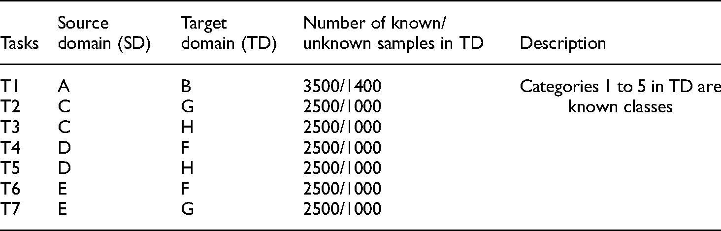
Compared with case 2 and case 3, case 1 has more training data and test data, so case 1 is taken as an example to analyze the fault diagnosis performance of the proposed model under cross-working conditions. The dataset in Case 1 is reorganized into domains as shown in Table 7. The CDFD tasks are shown in Table 8.

Table 7.

Information of each domain in case 1.

Domains	Load speed (×100r/min)	Categories (labels)	Number of samples
A	1/3/5/7/9/11/13/15	1/2/3/4/5	8 × 5 × 100 = 4000
B	2/4/6/8/10/12/14	1/2/3/4/5/6/7	7 × 7 × 100 = 4900
C	1/2/3/4/5	1/2/3/4/5	5 × 5 × 100 = 2500
D	6/7/8/9/10	1/2/3/4/5	5 × 5 × 100 = 2500
E	11/12/13/14/15	1/2/3/4/5	5 × 5 × 100 = 2500
F	1/2/3/4/5	1/2/3/4/5/6/7	5 × 7 × 100 = 3500
G	6/7/8/9/10	1/2/3/4/5/6/7	5 × 7 × 100 = 3500
H	11/12/13/14/15	1/2/3/4/5/6/7	5 × 7 × 100 = 3500

Table 8.

The cross-domain fault diagnosis (CDFD) tasks.

Tasks	Source domain (SD)	Target domain (TD)	Number of known/unknown samples in TD	Description
T1	A	B	3500/1400	Categories 1 to 5 in TD are known classes
T2	C	G	2500/1000
T3	C	H	2500/1000
T4	D	F	2500/1000
T5	D	H	2500/1000
T6	E	F	2500/1000
T7	E	G	2500/1000

We compared the proposed method H-CNN with CNN-2D and CNN-1D on the above seven CDFD tasks. The comparison results are shown in Figure 19. In Figure 19, H-CNN performs better than CNN-2D to classify known faults on tasks T2, T3, T4, and T6. For identifying unknown fault, H-CNN outperforms CNN-2D and CNN-1D in all seven tasks. At the same time, compared with CNN-2D and CNN-1D, H-CNN has smaller accuracy deviation, more stable performance, and higher reliability of diagnostic results.

Figure 19.

Comparison between H-CNN, CNN-2D, and CNN-1D for the seven cross-domain diagnosis tasks.

According to the trends shown in Figure 19, we grouped and analyzed the seven tasks according to the load speed of the SDs and TDs.

T2/T3/T5–T4/T6/T7: The average accuracy of T2/T3/T5 are lower than T4/T6/T7. In T2/T3/T5 tasks, the load speeds of the SDs are slower than that of the TDs. T4/T6/T7 tasks are just the opposite.

T2/T3–T6/T7: The average accuracy of T3 is lower than T2 while the accuracy of T7 is higher than T6. When the load speed of the SD is lower than that of the TD, the greater the difference between the speeds, the lower the accuracy. Conversely, the greater the difference between the speeds, the higher the accuracy.

T1–T2/T3/T4/T5/T6/T7: Compared with other tasks, T1 has the smallest difference between the working conditions of the TD and the SD, so the accuracy of T1 is higher than that of other tasks, which is in line with common sense.

Based on the above analysis, we guess that the fault features under high-speed conditions are more compatible than those under low-speed conditions. To further verify this conjecture, we independently trained and tested the data of each working condition. The results are shown in Figure 20. It is obvious that in the cylindrical roller bearing data set, the classification accuracy of low-speed conditions is always less than that of high-speed conditions. Under the test conditions of 100 r/min and 200 r/min, the classification accuracy of the known dataset is 86.39% and 90.47%, respectively. But it achieves to about 99% under the higher speed conditions. One possible reason is that the sampling frequency (20 khz) is too high, while the data length of the sample (3600) is too short. When the time domain signal is converted to the angle domain signal and the operating condition is 100 r/min, the rolling bearing rotates only 0.3 turns. Considering the fault frequency of rolling bearings, the fault characteristics are not obvious under the limited data length. It is difficult to extract useful features at low speeds. But when the proposed method H-CNN is utilized, the classification accuracy is improved under both low-speed conditions and high-speed conditions. This shows that the method proposed in this article can effectively enhance CNN's perception of less fault information.

Figure 20.

The accuracy of CNN and H-CNN under different operating conditions: (a) The accuracy for the classes which are trained and (b) the accuracy for the classes which are not trained.

It can be seen from the calculation method of Huffman pooling that Huffman pooling fully considers the impact of each value in the filter. In order to intuitively show that Huffman pooling can weaken the common components of signals and strengthen the impact components, we calculate the HACL directly on the original signal and then transform the signal into 2D image. As shown in Figure 21, a raw signal is converted into 2D image by two different methods. It can be seen that HACL has a good capability of noise reduction. So the Huffman pooling method can effectively improve the noise reduction ability of CNN and the sensitivity of CNN to the shock component in the signal.

Figure 21.

A raw signal converted into 2D image by different methods.

Case 2: Deep groove ball bearing

The images ( $60\times 60$ ) converted from deep groove ball bearing raw signals are shown in Figure 22.

Figure 22.

6312 deep groove ball roller bearing raw signals conversion results: (a) Inner race with breakage fault, (b) outer race with breakage fault, (c) retainer with breakage fault, and (d) ball with wear failure.

As shown in Table 4, the training data contains four classes of data and the testing data contains five classes of data. The accuracy of the recognition is defined as follows: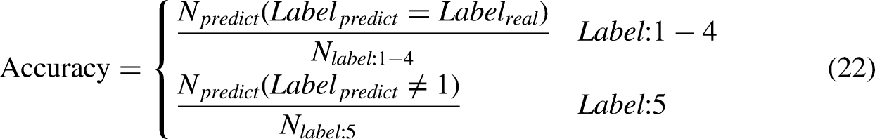

$$\mathrm{Accuracy}=\{\begin{array}{cc}{\displaystyle \frac{N_{predict}(Labe{l}_{predict}=Labe{l}_{real})}{N_{label:1-4}}}& Label:1-4\\ {\displaystyle \frac{N_{predict}(Labe{l}_{predict}\ne 1)}{N_{label:5}}}& Label:5\end{array}$$

(22)

The results of case 2 are shown in Table 9.

Table 9.

Comparison result of Huffman-convolutional neural network (H-CNN) and other methods in case 2 (%).

Methods	Average accuracy
	Known/Unknown
H-CNN	98.62/95.27
CNN-2D	98.35/91.58
CNN-1D	90.74/82.29
DBN	85.48/70.43
LSTM	93.24/74.28
ResNet	91.82/78.93
RF	85.74/76.53
KNN	77.68/63.59
SVM	86.25/74.85
ANN	70.24/63.65

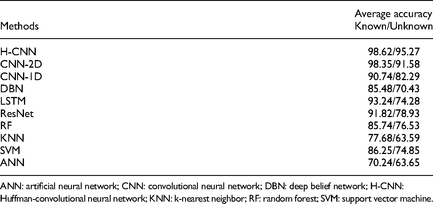
ANN: artificial neural network; CNN: convolutional neural network; DBN: deep belief network; H-CNN: Huffman-convolutional neural network; KNN: k-nearest neighbor; RF: random forest; SVM: support vector machine.

It can be seen that the proposed H-CNN method obtains a better result compared with other methods in this case. The mean prediction accuracy is as high as 98.62% for known data and 95.27% for unknown data. For the known data, the prediction results of CNN-2D, CNN-1D, DBN, LSTM, ResNet, RF, KNN, SVM, and ANN are 98.35%, 90.74%, 85.48%, 93.24%, 91.82%, 85.74%, 77.68%, 86.25%, and 70.24%, respectively. As for unknown data, the prediction results of CNN-2D, CNN-1D, DBN, LSTM, ResNet, RF, KNN, SVM, and ANN are 91.58%, 82.29%, 70.43%, 74.28%, 78.93%, 76.53%, 63.59%, 74.85%, and 63.65%, respectively. Table 9 shows that the proposed H-CNN has a good capability in fault diagnosis. Since there are fewer fault types in this case than in Case 1, the recognition accuracy, in this case, is generally higher than that in case 1.

The confusion matrices of different methods in case 2 are shown in Figure 23. SVM, CNN, and H-CNN mistake the data of fault (Figure 23(d)) as normal data probability is 25.15%, 8.42%, and 4.73%, respectively.

Figure 23.

The confusion matrices of different methods in case 2: (a) SVM, (b) CNN, and (c) H-CNN.

Case 3: Gearbox system

The images ( $60\times 60$ ) converted from gearbox system raw signals are shown in Figure 24.

Figure 24.

Gearbox raw signals conversion results.

As shown in Table 5, the training data contains seven classes of data and the testing data contains nine classes of data. The accuracy of the recognition is defined as follows: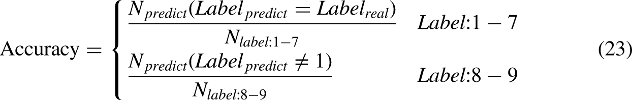

$$\mathrm{Accuracy}=\{\begin{array}{cc}{\displaystyle \frac{N_{predict}(Labe{l}_{predict}=Labe{l}_{real})}{N_{label:1-7}}}& Label:1-7\\ {\displaystyle \frac{N_{predict}(Labe{l}_{predict}\ne 1)}{N_{label:8-9}}}& Label:8-9\end{array}$$

(23)

The results of case 3 are shown in Table 10.

Table 10.

Comparison result of Huffman-convolutional neural network (H-CNN) and other methods in case 3 (%).

Methods	Average accuracy
	Known/Unknown
H-CNN	99.79/96.32
CNN-2D	98.63/93.74
CNN-1D	93.13/80.42
DBN	80.67/71.38
LSTM	90.28/75.14
ResNet	92.44/69.58
RF	83.57/78.62
KNN	75.34/62.97
SVM	89.76/77.25
ANN	71.38/65.82

ANN: artificial neural network; CNN: convolutional neural network; DBN: deep belief network; H-CNN: Huffman-convolutional neural network; KNN: k-nearest neighbor; RF: random forest; SVM: support vector machine.

From Table 10, the proposed H-CNN method obtains a better result compared with other methods in this case. The average prediction accuracy is as high as 99.79% for known data and 96.32% for unknown data. For the known data, the prediction results of CNN-2D, CNN-1D, DBN, LSTM, ResNet, RF, KNN, SVM, and ANN are 98.63%, 93.13%, 80.67%, 90.28%, 92.44%, 83.57%, 75.34%, 89.76%, and 71.38%, respectively. As for unknown data, the results of CNN-2D, CNN-1D, DBN, LSTM, ResNet, RF, KNN, SVM, and ANN are 93.74%, 80.42%, 71.38%, 75.14%, 69.58%, 78.62%, 62.97%, 77.25%, and 65.82%, respectively.

The confusion matrices of different methods in case 3 are shown in Figure 25. SVM, CNN, and H-CNN mistake the data of fault (chip 2a) as normal data probability is 24.47%, 5.14%, and 3.54%, respectively. As for the fault (chip 1a), the misjudgment rates are 21.03%, 7.38% and 3.82%, respectively.

Figure 25.

The confusion matrices of different methods in case 1: (a) SVM, (b) CNN, and (c) H-CNN.

In addition, as can be seen from Figure 25, since chip 2a and chip 1a belong to the same type of faults with different degrees, the three methods mentioned above are easy to identify them as chip-*a type. Moreover, the closer the fault degree is, the less accurate these identification methods can be in distinguishing them.

Conclusion

In this research, we mainly discuss the generalization ability of CNN when handling fault diagnosis tasks with more test data categories than training data categories. A new fault diagnosis method called H-CNN is proposed based on CNN and Huffman pooling for rotating assembly and a new objective function based on the mixed loss is designed for the H-CNN. Then, we apply the proposed method in three different datasets. To verify the effectiveness of the method proposed in this article, comparisons are made with some other state-of-the-art methods, including CNN-2D, CNN-1D, DBN, LSTM, ResNet, RF, KNN, SVM, and ANN. The average accuracy of classifying known faults under various working conditions are H-CNN—97.93%, CNN-2D—98.26%, CNN-1D—92.14%, DBN—84.84%, LSTM—91.71%, ResNet—92.37%, RF—83.65%, KNN—75.14%, SVM—84.55%, and ANN—70.02%. The average accuracy for unknown anomaly detection under various working conditions are H-CNN—94.51%, CNN—2D-91.33%, CNN—1D-80.34%, DBN—71.68%, LSTM—71.66%, ResNet—74.25%, RF—75.54%, KNN—64.13%, SVM—74.15%, and ANN—63.03%. Compared with other methods, the results show that the proposed method has a good performance in improving the accuracy of classifying the known data and detecting the unknown fault data as anomaly data. At the same time, compared with other advanced domain generalization methods, the proposed method does not need to adopt other complex auxiliary methods to extract fault features in advance, and only needs to use the simplest CNN network structure to achieve better generalization effect. Therefore, the method proposed in this article has a good development prospect in the field of fault diagnosis of rotating component of the mechanical equipment.