Sage Journals: Discover world-class research

Abstract

Rivets are used to assemble layers in the air intakes, fuselages, and wings of an aircraft. After a long time of working under extreme conditions, pitting corrosion could appear in the rivets of the aircraft. The rivets could be broken down and thread the safety of the aircraft. In this paper, we proposed an ultrasonic testing method integrated with convolutional neural network (CNN) for the detection of corrosion in the rivets. The CNN model was designed to be lightweight enough to be able to run on edge devices. The CNN model was trained with a very limited sample of rivets, from 3 to 9 artificial pitting corrosive rivets. The results show that the proposed approach could detect up to 95.2% of pitting corrosion using experimental data with three training rivets. The detection accuracy could be improved to 99% by nine training rivets. The CNN model was implemented and ran on an edge device (Jetson Nano) in real-time with a small latency of 1.65 ms.

Keywords

Ultrasonic testing pitting corrosion in aircraft convolutional neural network ResNet AI on edge devices

Introduction

Aircraft structures such as air intakes, fuselages, and wings are multilayer structures made of thin-aluminum layers. The thin aluminum layers are assembled by a lot of rivets, which help the structure to be lightweight and persistent. However, the working conditions of the aircraft are extreme, with a wide range of temperatures, high pressure, vibrations, and repeated loads during the operation. The rivet and its countersunk sites are getting high-pressure concentration and potential areas for the attachment with salinity and moisture.¹ There are two kinds of damages that are usually reported in those areas, which are corrosion in the hidden sites of aluminum layers and pitting corrosion/crack in the rivet head.^2,3 Therefore, the nondestructive testing (NDT) methodology is widely used in the inspection service to ensure the integrity of the aircraft.

Several common NDT methods, such as magneto-optical imaging (MOI), eddy current testing (ECT), and magnetic camera, have been developed and used in the inspection of aircraft nowadays. MOI system works based on the Faraday's effect of the interaction between electromagnetic field and polarized light. As eddy current flows distorted by damages, electromagnetic fields will be produced and change the angle of the polarized light plane. Thus, the presence of damage could be observed in the film. The film has a large area and high spatial resolution, so the MOI system could visualize a large area of the aircraft.^4,5 However, the MOI system has only white/black color, which limits the evaluation of damage size and damage location. Alternatively, ECT systems have been widely used recently and are known as the standard NDT method in the inspection of aircraft structures. Instead of observing the changes in the electromagnetic field by the polarized light beam, ECT system observes the changes in the sensing coil's impedance due to the distorted eddy current. The ECT sensor usually has an exciting coil to supply an electromagnetic field and a sensing (differential mode) coil or just a single coil for both exciting and sensing tasks (absolute mode). These ECT systems provide a high sensitivity to surface and subsurface damage and can detect hidden corrosion in the layers of the multilayer structure.^6-8 The exciting and sensing coils could be arranged in an eddy current array probe to detect a large area of the aircraft and be commercialized using in the practical (e.g. Ommiscan system Olympus, ECA system Eddyfi).^9,10 However, the sensing coil measures the rate change of the electromagnetic field, which requires a high frequency of the exciting source in a high-sensitivity probe. The high operating frequency of the probe decreases the skin depth of the eddy current penetration in the layers; thus, it limits to detect the deep damage under the layer's surface. To overcome this limitation, magnetic camera has been developed, in which they use magnetic sensors such as Hall or giant magneto-resistance sensors to directly measure the changes of the magnetic field around the damage.^11–13 The magnetic camera could be operated at lower frequency. The exciting source could be a single large yoke-type magnetic source, and the magnetic sensor could be arranged in a dense area for a high spatial resolution of the measurement. The magnetic camera could detect the hidden corrosion in the first layer or second layer of the aircraft. It is also possible to evaluate the size, such as volume and depth of the corrosion by the system.¹¹ All of these systems work on the same principle of eddy current distribution on the multilayer structure. The magnetic source produces an electromagnetic field into the conductive layers; then, an eddy current is induced in the layer. If the layer has damage, the eddy current will be distorted and produces a secondary electromagnetic field. The damage could be detected by measuring the secondary magnetic field via a polarized light beam in the MOI system, the impedance of the sensing coil in the ECT system, or the magnetic field value in the magnetic camera. These systems could provide good detectability of hidden corrosion in different layers; however, they could not detect the pitting corrosion inside the rivet. The main reason is that the fastener hole, where the rivet is located, is considered as a large defect, producing much stronger distortion on the eddy current than the pitting corrosion in the rivet. Thus, the secondary electromagnetic field from the pitting corrosion is not distinguished from the measurement results.

Another NDT method, such as ultrasonic testing (UT) could be used to overcome the limitation of ECT's based systems. The UT system supplies an ultrasonic wave into the rivet; if there is corrosion inside the rivet, the ultrasonic wave will be reflected back and measured.^14–17 The operating principle is not only much simple than the ECT-based systems but it also suffers from some difficulties such as: 1) the ultrasonic wave could only efficiently propagate in the continuous mediums which require the supplement of coupling liquid (e.g. water) and could not detect the hidden corrosion in the second or third layer of the structure due to the air-gap between the layers, 2) the reflected ultrasonic wave at the rivet area in the multilayer structure is complex with multiple noises from the rivet head, layer surface, hidden corrosion in a layer, layer's air gap, etc.; thus, the analysis of the measured signal is difficult. Previous researchers have tried to solve the first problem by incorporating a magnetic camera with a UT probe. The magnetic camera is used for detecting the hidden corrosion in the layers, and the UT probe is used to detect the pitting corrosion inside the rivet. The magnetic camera is also used to detect the center of the rivet for guidelines for the scanning of the UT probe.¹⁸ However, the signal analysis of the UT probe for pitting corrosion detection is still limited due to its complexity.¹⁹

To overcome the limitation, we proposed a deep neural network for the detection of pitting corrosion in the rivet using UT signals. Deep neural network is a powerful machine-learning technique that has been developed and applied in many automation applications such as automatic metallic surface defect segmentation,²⁰ self-learning in robotics,²¹ object identification,^22,23 human-machine interaction,²⁴ natural language processing,^25,26 and machine translation.²⁷ The network is capable of capturing extracting patterns of the signal in the training phase and generalizing to new unseen signals. In this research, we developed a convolutional neural network (CNN) model to deal with several problems: improving the probability of detection (POD) of pitting corrosion of the UT system; CNN model is lightweight and could be implemented in real-time on edge devices (e.g. Jetson Nano); The CNN model could be trained with very few data (i.e. several rivets with/without pitting corrosion). To verify the performance of the proposed approach, we investigated the UT system with artificial pitting corrosion with different scan locations of the UT probe and different sizes of corrosion in depth and length. The UT system could detect up to 95.2% of corrosion with signal is amplified via an amplifier requring just 5099 parameters, and 1.65 ms to process.

Ultrasonic testing system

Principle

A general block diagram of the UT system is shown in Figure 1. The UT probe is used for scanning the surface of the multilayers specimen which is assembled by rivets. A membrane filled with water is attached at the head of the UT to enable the ultrasonic wave to propagate into the specimen during the scan. The corrosion in the layers and rivet could be detected by analyzing the reflected wave signal. The pulser/receiver board supplies pulses for the UT probe and preprocess the reflected wave. The received signal is amplified via an amplifier, and noise is reduced by a band-pass filter. The signal is then digitalized by an analog-to-digital converter (ADC) in the digitizer module. In addition, generated pulses are synchronized with the received signal by the trigger generated from the digitizer. The ADC signal is then transformed into the frequency domain by short-time Fourier transform (STFT) and subsequently fed into a CNN model for corrosion detection. In this paper, the CNN model is designed to be lightweight enough to be implemented in edge devices such as the Jetson Nano board.

Figure 1.

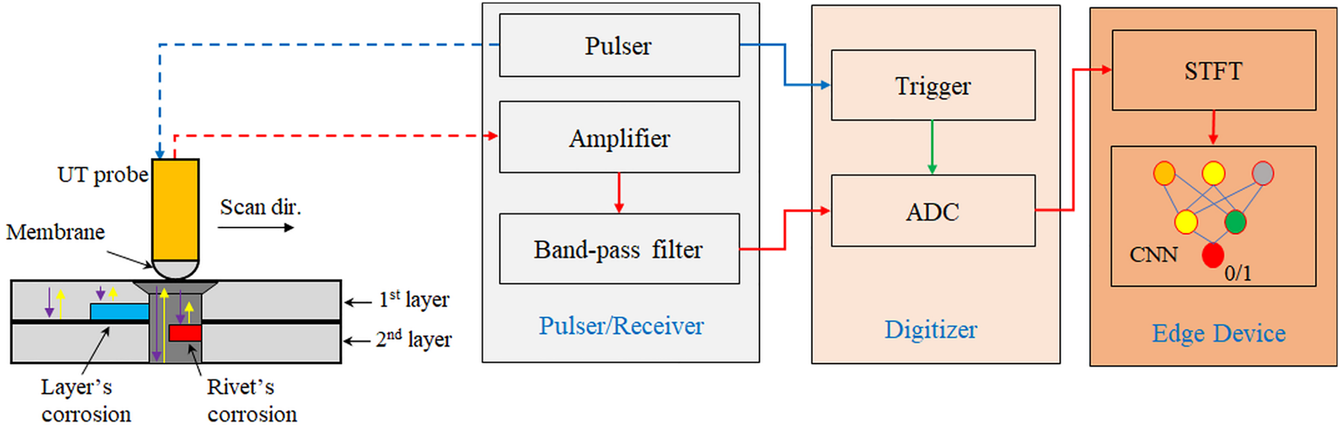
Block diagram of the ultrasonic testing system.

Experimental setup

Figure 2 shows the experimental setup and equipment of the UT system. The UT probe is attached to a precise XYZ stage scanner. During the scan process, the membrane of the UT probe is contacted with the surface of the multilayer, which allows the propagation of the ultrasonic wave into the multilayer. The membrane is filled with water. With the use of the water membrane, there is no need to supply couplant material during the scan of the UT probe, simplyfing the system. However, this also causes the received signal to be more complicated due to the lift-off variation and deformation of the membrane. The spring is positioned in the backside of the probe to protect the UT probe from collision with the specimen during the scan. The UT probe has a spot-welding type probe with a center frequency of 13.3MHz (V2335). A pulser/receiver (PCR50) was used to supply pulse to the UT probe and also obtain reflected signals from the surface/bottom layer and corrosion. The pulse repetition rate was set at 0.1 s, enough for the full propagation of the ultrasonic wave into the rivet and the multilayer. The gain of the amplifier was set at 20 dB, and the band-pass filter was set from 0.3 to 25 MHz. The filtered signal is then digitized by a high-speed NI USB 5133 at 100 MHz sampling rate. The digitizer is triggered by a pulse generated from the PCR50 at 100 Hz. The scan speed of the UT probe is about 6 mm/s.

Figure 2.

Experimental setup and equipment of the ultrasonic testing system.

Figure 3.

Scan positions and directions of the UT probe on the rivet head.

A multilayer specimen includes two aluminum layers (Al 2024) and is assembled by 25 aircraft-type rivets (Air Force and Navy standard). The rivet has a length of 9.45 mm, a head diameter of 5.85 mm, and a body diameter of 3.95 mm as illustrated in Figure 3. This is a flat specimen simulated for air-intake aircraft structure. Among 25 rivets, there are 13 rivets that have artificial corrosion, and 12 rivets have no corrosion. The corrosion has length (L) of 1.0, 1.35, 2.0, and 2.65 mm, depth (d) of 1.0, 1.5, and 2.0 mm, and at one side and both sides of the rivet body. Each rivet was scanned in four directions: forward, backward, left, and right at five different lines at 0.5 mm interval. This setting is for taking the effect of the scan directions relative to the corrosion location and the detection possibility of the UT probe if the scan line is not at the center of the rivet in the real scenes into account.

Data preparation

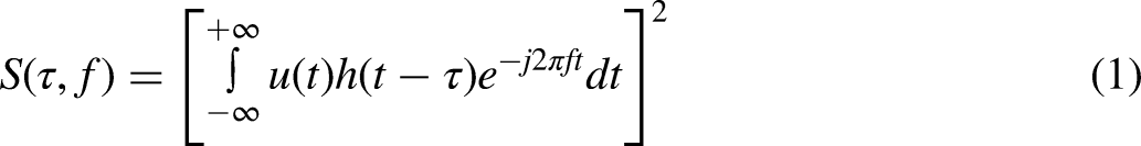
In each scan line of the UT probe, the reflected ultrasonic signal is acquired and transformed into a spectrogram by STFT, as described in equation (1).¹⁹ By summary of the spectrogram in the UT probe frequency band as described in equation (2), the spectrogram of the scan signal is formed and helps visualize the components of signal clearer, as shown in Figure 4. The first layer's surface, repetition of the first layer bottom, and corrosion in the fastener site are on the far-side of the first layer, and the rivet head could be identified clearly. With the center frequency of the UT probe at 13.3 MHz, the bandwidth is taken from 12.3 MHz (f_a) to 14.3 MHz (f_b). The spectrogram signals will be used as the input for the CNN model in the later section:

S (τ, f) = {[\int_{- \infty}^{+ \infty} u (t) h (t - τ) e^{- j 2 π f t} d t]}^{2}

(1)

B (τ, x) = \frac{1}{f_{a} - f_{b}} \sum_{f_{b}}^{f_{a}} S (τ, f)

(2)

Figure 4.

A sample of received-absolute signal in waterfall plot and spectrogram signal.

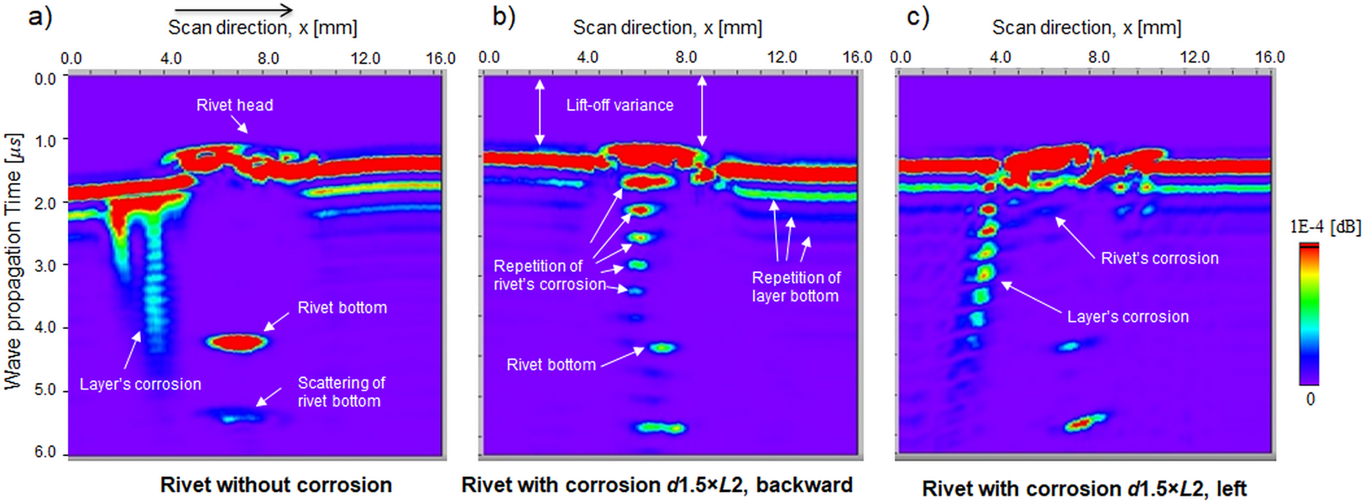
Figure 5 shows the spectrogram of the scan signal for a rivet with and without corrosion. The repetition of the rivet's corrosion signal could be observed under the rivet head clearly, as shown in Figure 5(b). And with the existence of the corrosion, the rivet's bottom signal decreases because the corrosion reflects a part of the ultrasonic wave. However, in the left-scan direction, the rivet's corrosion is harder to be observed because it has low intensity and is connected with the layer's corrosion. In addition, during the scan, the deformation of the water membrane produces the lift-off variance and the wave propagation direction variance (not 90° with the specimen surface), making the received signal more complicated. Therefore, we developed a CNN model for fast and efficient detection of the rivet's corrosion in various situations of the corrosion signals. It is noted that the layer's corrosion signal is not the detection target of this research because the signal is so clear to be observed by the necked eye and could be easily detected by a simple algorithm. The layer's corrosion is considered as the noise contribution to the rivet's corrosion because they are sometimes connected together.

Figure 5.

A sample of the rivet with (a) and without (b, c) corrosion in the spectrogram plots.

There are 13 rivets with corrosion and 12 rivets without corrosion in the experiment. Each rivet was performed in four scan directions on five lines, as mentioned in the previous sections.¹⁹ A window of 512 × 96 was 10 times randomly captured the UT spectrogram scan images to enrich the number of the dataset and to cover more situations of the UT signal, especially when there is a variant of the lift-off and the wave propagation angle during experiments. Totally, there are 5000 UT spectrogram images with and without rivet's corrosion. The later sections will investigate the effect of the number of training datasets on the prediction accuracy of the CNN model.

Convolutional neural network

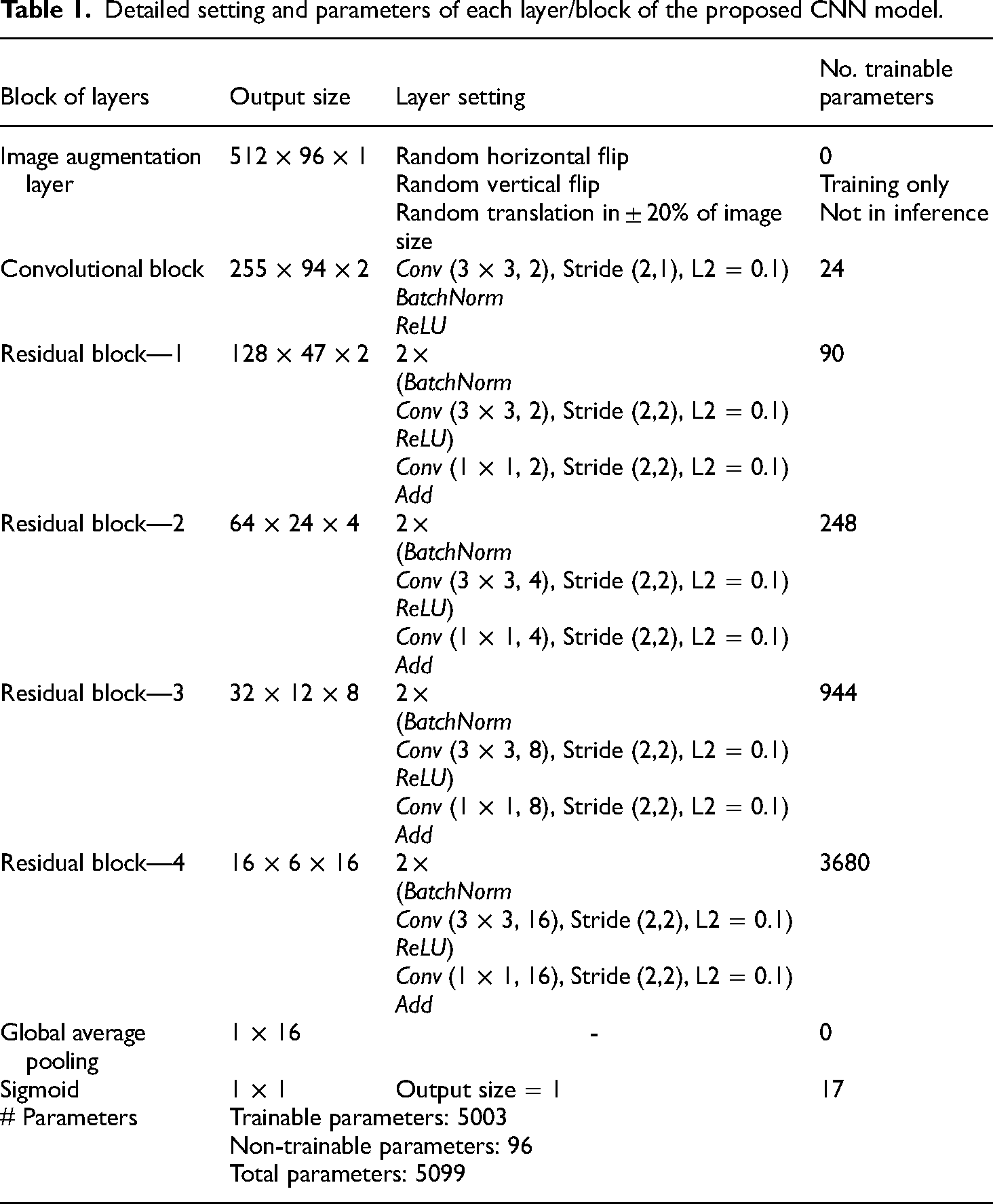
The structure of the CNN model is shown in Figure 6. The scan spectrogram ultrasonic image with the size of 512 × 96 is the input (X) to the model, and the binary output is the rivet with (1) or without (0) corrosion. The CNN model is a variant of the residual network structure, that has one convolutional block, four residual blocks, one global average pooling (GAP), and a sigmoid layer for classification. The convolutional block is used to first extract the local correlation of the spectrogram, reduce half spatial resolution in the scan direction but keep the data information by the double expansion of the output channels. It has a linear convolutional layer with the kernel size of 3 × 3, strides of (2,1), and the BatchNorm layer is used before the nonlinear ReLU activation. The output of the convolutional block is expressed in equation (3):

Y_{c o n v} = R e L U (B a t c h N o r m (C o n v 2 D (X)))

(3)

Figure 6.

Convolutional neural network structure.

The output of $Y_{c o n v}$ the convolutional block is fed in a series of four residual blocks. Each residual block reduces half of the spatial resolution in both the scan and the wave propagation direction but doubles the output channel. The residual block has two main convolutional blocks, but each has different sequences of the layer as the first convolutional block; this layer sequence is the best for the residual block, which has been investigated and reported in previous research.^28,29 The convolutional layer has the kernel size of 3 × 3 and strides of (2,2). Especially, there is a convolutional layer with a kernel size of 1 × 1 bridges from the input to the mainstream output of the residual block. The convolutional layer 1 × 1 reduces half spatial resolution and doubles the channel for matching with the mainstream output's size. The outputs are summarized together so that if the mainstream is hard to learn the data, the input is just passed the residual block without changing its information, and the later block might be learned better. The output of the residual block is expressed in equation (4). The residual term was further extended to use in other efficient models such as Inception-Resnet and DenseNet model. Inception-ResNet (e.g. V4) model is an improvement of the orginal Inception model with the residual term. However, the use of multiple kernels at a the same time in the Inception blocks results in exceeding peak-memory available on the majority of edge devices.³⁰ In the DenseNet model, all the dense blocks are connected directly with each other.³¹ However, this dense connection also requires storing the output activation of every block that would increase the memory usage. So, this concept was not used in our proposed model:

Y_{r e s i d u a l} = B a t c h N o r m (R e L U (C o n v 2 D_{3 \times 3} (X))) + C o n v 2 D_{1 \times 1} (X)

(4)

The output of the last residual block is passed through a GAP which average the data in spatial resolution. Then, it passes through a Sigmoid layer for the corrosion detection result. There is no fully connected layer in the last layers; thus, the number of parameters is minimized. In addition, an augmentation layer is applied during the training process to raise the number of training samples but not used in the inference process. We applied random vertical flip, horizontal flip, vertical translation (20%), and horizontal translation (20%). In addition, to avoid overfitting, we applied L2-regularization in each convolutional block with the weight of 0.1. These regularization parts are added to the cross-entropy loss function of the model. The detailed sequence and size of the layers are shown in Figure 6 and Table 1. The model is lightweight with only 5099 parameters in total, including 5003 trainable and 96 nontrainable parameters.

Table 1.

Detailed setting and parameters of each layer/block of the proposed CNN model.

Block of layers	Output size	Layer setting	No. trainable parameters
Image augmentation layer	512 × 96 × 1	Random horizontal flip Random vertical flip Random translation in ± 20% of image size	0 Training only Not in inference
Convolutional block	255 × 94 × 2	Conv (3 × 3, 2), Stride (2,1), L2 = 0.1) BatchNorm ReLU	24
Residual block—1	128 × 47 × 2	2 × (BatchNorm Conv (3 × 3, 2), Stride (2,2), L2 = 0.1) ReLU) Conv (1 × 1, 2), Stride (2,2), L2 = 0.1) Add	90
Residual block—2	64 × 24 × 4	2 × (BatchNorm Conv (3 × 3, 4), Stride (2,2), L2 = 0.1) ReLU) Conv (1 × 1, 4), Stride (2,2), L2 = 0.1) Add	248
Residual block—3	32 × 12 × 8	2 × (BatchNorm Conv (3 × 3, 8), Stride (2,2), L2 = 0.1) ReLU) Conv (1 × 1, 8), Stride (2,2), L2 = 0.1) Add	944
Residual block—4	16 × 6 × 16	2 × (BatchNorm Conv (3 × 3, 16), Stride (2,2), L2 = 0.1) ReLU) Conv (1 × 1, 16), Stride (2,2), L2 = 0.1) Add	3680
Global average pooling	1 × 16	-	0
Sigmoid	1 × 1	Output size = 1	17
# Parameters	Trainable parameters: 5003 Non-trainable parameters: 96 Total parameters: 5099

Results and discussions

CNN model results

To train the CNN model, four rivets with corrosion and four rivets without corrosion corresponding to 32% of the total data were used; the other rivets (68%) were used for validating the model. We just deal with a few numbers of the data because this is generally a hard problem in the NDT field, where the data is scare and not easy to be collected. The training process follows a cross-validation approach, but the rivets are selected randomly five times. We used Adam optimizer with initial learning rate of 0.001 and reduced ten times if the validation loss does not decrease within five epochs. The convolutional parameters were initialized using He's strategy in which the truncated normal distribution center of 0 and standard deviation of $s q r t (2 / n u m b e r o f i n p u t u n i t s)$ . The model was trained on a high-performance computation with 2 × A100 GPU and 128G RAM. The training epochs are 200, and the batch size is 32 spectrogram images. The hyperparameters and training/validation dataset information are summarized in Table 2.

Table 2.

Summary of the training hyperparameters and datasets.

Hyperparameters/Datasets	Values
Model's parameters	5099
Optimizer	Adam
Learning rate	0.001
Learning rate decay if validation loss no decreases within 5 epochs	0.1
Initializer	He's strategy
Batch size	32
Training epochs	200
Save the best model on validation accuracy	Yes
Number of training dataset	1600 images (8 rivets)
Number of validation dataset	3400 images (17 rivets)
Training on HPC	2 Nvidia A100 GPU 128 GB RAM each GPU

Figure 7 shows the training loss and accuracy of training and validation dataset, and confusion matrix of the CNN model with the validation dataset. It seems that the model is warming up in the first few epochs. So, the model is not generalized to the validation dataset that the loss function is high, and the accuracy is so low. After that, the accuracy improves as the epoch increases to around 40, the model gets stable after that. The accuracy of the rivet with and without corrosion is 93.82% and 97.78%, respectively, thus the average accuracy is 95.68%. The rivets without corrosion are easier to detect because their signal patterns are not much different than in the case of rivets with corrosion which have different corrosion sizes. Figure 8 shows the t-SNE of the last layer, where the features are the output of the GAP layer. The features are represented by two first t-SNE components with different perplexities from 10 to 110. As the perplexity increases, the data points of each class are more condensed and separatable. And the result shows that the CNN model is efficient in extracting features of the ultrasonic spectrogram image.

Figure 7.

Training loss, accuracy of training and validation dataset, and confusion matrix of the CNN model with validation dataset (32% of total data).

Figure 8.

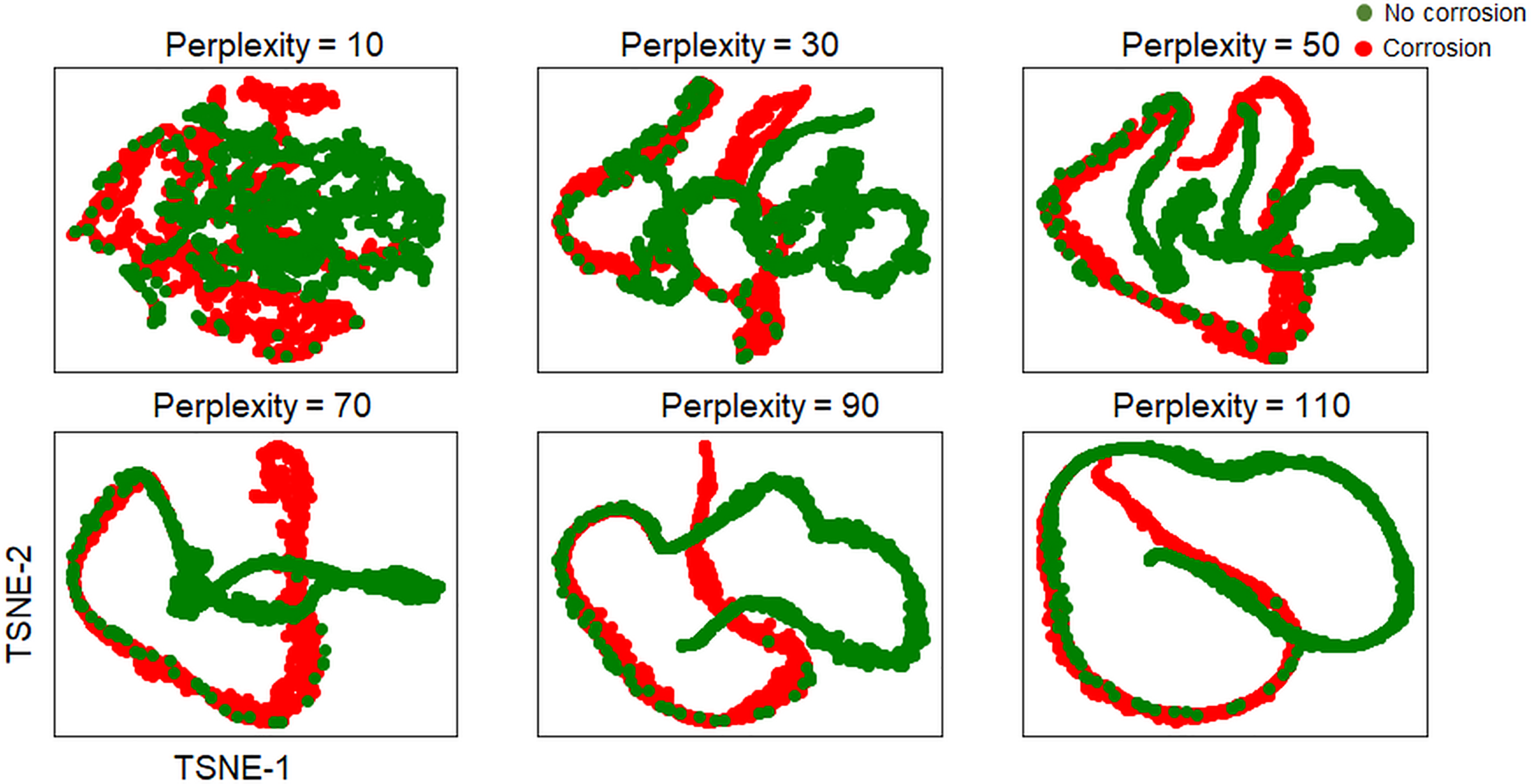
t-SNE distribution of the last layer (global average pooling) of the validation dataset.

Figure 9 shows some samples of the saliency map produced by the CNN model with Grad-CAM++ method.³² The high intensity of the overlayed images in the rivet with corrosion indicates the importance of the pixels that contribute to the prediction results. Those areas include the head of the rivet and the corrosion area. But the pixels of the saliency map of the rivet without corrosion are equal and small, which does not emphasize any area of the spectrogram image. This is different from the observation of the peak detection method in the previous study,¹⁹ in which only the corrosion area (rivet body) was analyzed. The CNN model provided high prediction accuracy; however, there are few cases in which the model gave wrong prediction results. The right side of Figure 9 shows the wrong detection of the corrosion with the Grad-CAM++. When the rivet has a true label of no-corrosion and the predicted label of corrosion, the Grad-CAM++ only focuses on the rivet's head, rivet's bottom, and multilayers but not on the rivet's body area. And when the rivet has a true label of corrosion and the predicted label of no-corrosion, the model could not find any data (e.g. in the rivet's body area) to give the right decision.

Figure 9.

Saliency maps produced by the CNN model with grad-CAM++ method.

Effect of the number of training data

To evaluate the effect of the number of the training dataset on the performance of the CNN model, the numbers of rivets with and without corrosion were selected from 1 to 9, corresponding to 8%–72% of the total dataset (the number of rivets with and without corrosion is same). The result in Figure 10 shows the increase in accuracy as the number of rivets increases. The average accuracy passes the peak-detection (PD) method¹⁹ (92.8%), with only three rivets having corrosion in the training dataset (95.2%). The accuracy increased and saturated at around 99%, with 8 and 9 rivets having corrosion. Similarly, the receiver operating curve is also better as the number of rivets in the training dataset increases, as shown in Figure 11.

Figure 10.

Prediction accuracy of the validation dataset versus the number of rivets in the training dataset.

Figure 11.

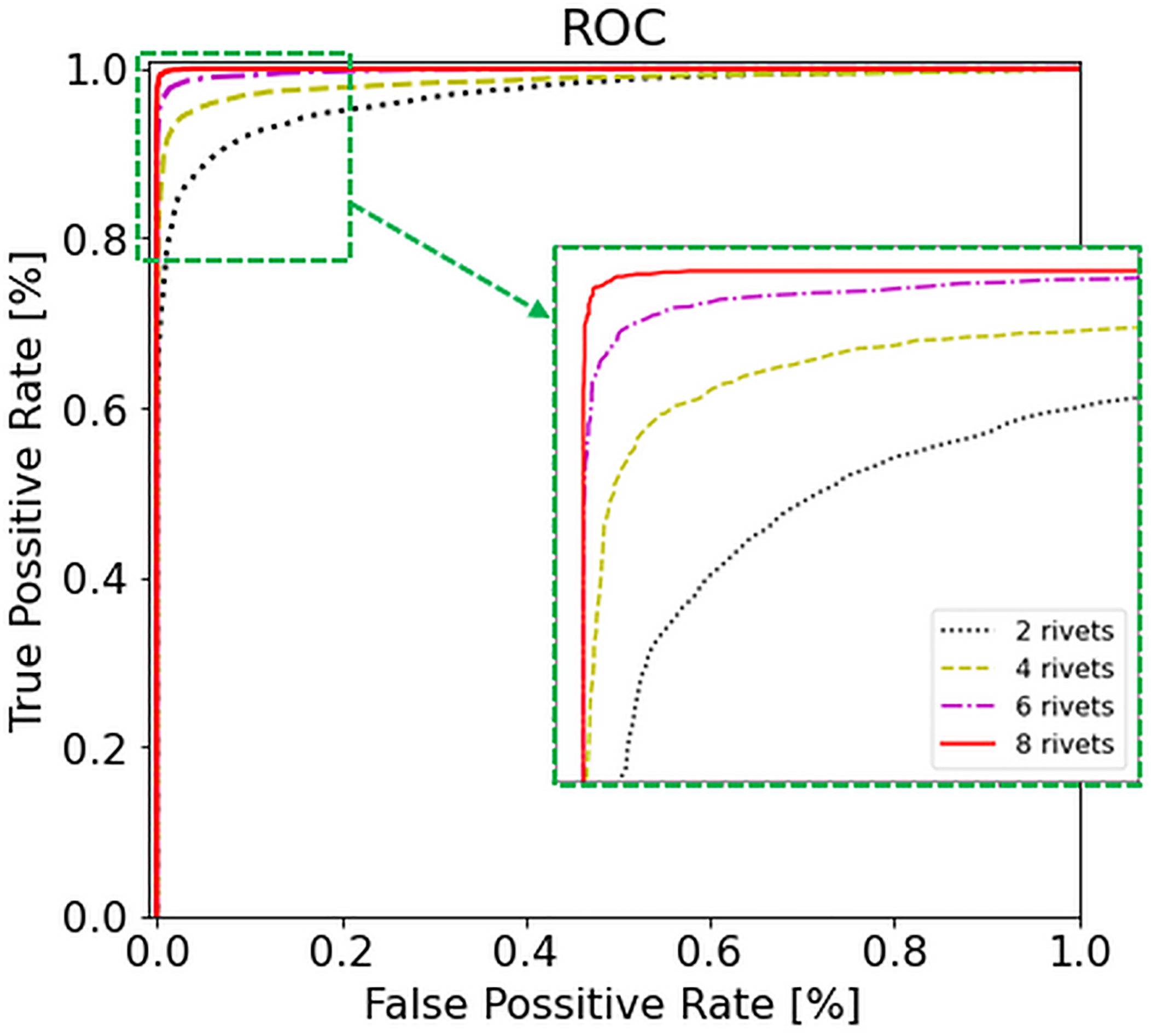
Receiver operating curves (ROC) with different numbers of rivets in the training dataset.

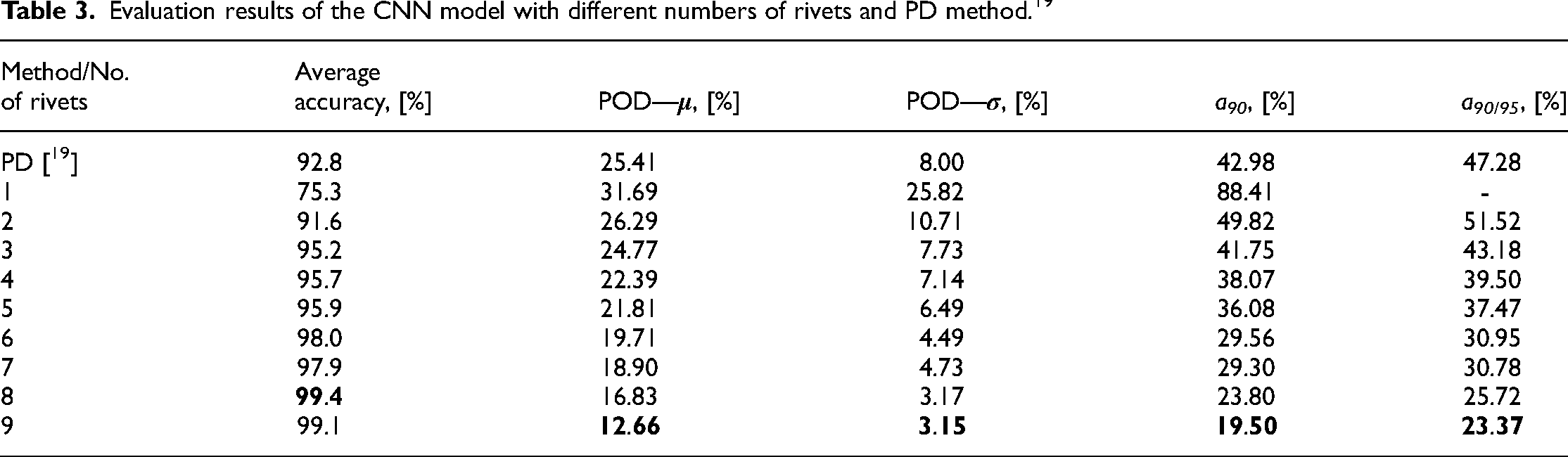
Figure 12 shows the POD of the CNN model with a different number of rivets in the training dataset and compares it with the PD method.¹⁹ The hit/miss data obtained from the prediction results were used with the logit model of the POD. The parameters of the POD curves, which are mean ( $μ$ ), standard deviation ( $σ$ ), size at 90% POD (a₉₀), size at 90% POD, and 95% confidence (a_90/95), were obtained from mh1823 software V.4.0.1.³³ The CNN model provides worst POD than the PD method¹⁹ when using only 1 or 2 rivets for training, but it is significantly improved when the number of rivets is higher. The accuracy of the model improved by 6.3% than the PD method when using 9 rivets for training. And the POD was also improved that the system got a₉₀ = 19.5% and a_90/95 = 23.37% which are about two times smaller than the PD method. The detailed evaluation results are shown in Table 3.

Figure 12.

Probability of detection (POD) produced by the CNN model with different number of rivets (2, 4, 6, and 8) in the training dataset and the result from the peak-detection method.¹⁹

Table 3.

Evaluation results of the CNN model with different numbers of rivets and PD method.¹⁹

Method/No. of rivets	Average accuracy, [%]	POD— $μ$ , [%]	POD— $σ$ , [%]	a₉₀, [%]	a_90/95, [%]
PD [¹⁹]	92.8	25.41	8.00	42.98	47.28
1	75.3	31.69	25.82	88.41	-
2	91.6	26.29	10.71	49.82	51.52
3	95.2	24.77	7.73	41.75	43.18
4	95.7	22.39	7.14	38.07	39.50
5	95.9	21.81	6.49	36.08	37.47
6	98.0	19.71	4.49	29.56	30.95
7	97.9	18.90	4.73	29.30	30.78
8	99.4	16.83	3.17	23.80	25.72
9	99.1	12.66	3.15	19.50	23.37

Running on an edge device

To investigate the performance of the CNN model on edge devices, we implemented the model in the NVIDIA Jetson Nano development board. The device is a small, powerful, and energy efficient (∼5 W) embedded computer. Jetson Nano has a GPU that helps the device inference run in parallel for fast prediction.³⁴ The CNN model was built and trained using the TensorFlow framework. With a total of 5099 parameters, the original model size in TensorFlow is 1.32 MB, which is not the optimized size. We then converted the TensorFlow model to Open Neural Network Exchange Format (ONX), a format representing any machine learning and deep learning model from various frameworks such as PyTorch, TensorFlow, Keras, SAS, and MATLAB. Then, the model was further converted to optimized TensorRT (TRT) format for running efficiently on the Jetson Nano board. We fully converted the model to 32 and 16 floating format for the parameters and intermidiate activation. The Multiply-Add Operations (MACs) and Floating-Point Operations Per Second are 2.13 million and 4.26 million, respectively. The throughput and latency is about 604 fps and 1.65 ms. The model size was significantly reduced to 351 KB ( × 3.76) and 157 KB ( × 8.4) for the float32 and float16 formats. And the Peak-Memory when running the model (only) is 19 MB and 15 MB for float32 and float16 format, respectively. In addition, the accuracy of the model was slightly higher than the original TensorFlow model by about 0.21%. The detailed information is listed in Table 4. It is noted that the accuracy sometimes could slightly decrease or increase due to the data type conversion process. Besides, the UT probe has a pulse repetition frequency of 100 Hz, which takes 10 ms for an ultrasonic wave acquisition. Thus, the CNN model could be running in real-time on the Jetson Nano and delivers real-time results for corrosion detection.

Table 4.

Specification of the proposed CNN model running on Jetson Nano device.

Model parameters—data types in TRT	MACs	FLOPS	Peak-Memory (only model at runtime)	Validation accuracy improvement	Throughput	Latency	Model size
Float32	2.13 M	4.26 M	19 MB	0.21%	608 fps	1.64 ms	351 KB
Float16	2.13 M	4.262 M	15 MB	0.21%	604 fps	1.65 ms	157 KB
The original model in TensorFlow size: 1.32 MB
Model total parameters: 5099

Conclusions

This paper proposed an NDT method for the inspection of pitting corrosion in rivets of multilayer structures. A UT-integrated membrane probe was used for scanning the surface of the rivets. A CNN model was developed and implemented on an edge device (Jetson Nano) for processing the ultrasonic signal and real-time detection of the corrosion. The CNN model was designed to be lightweight, low memory usage, and fast inference time that could improve the POD and real-time corrosion detection. The CNN model also requires very few rivet samples for training. We demonstrated the proposed system with artificial pitting corrosion having different depths and lengths on the rivets of an aircraft structure. The result shows that the CNN model could detect corrosion with a surface area of 23.37% of the rivet body cross-section with a 90% POD and 95% confidence intervals. The corrosion size was half of the previous research (47.28%).¹⁹ Furthermore, even with only three corrosive rivets for training, the model could provide (43.18% surface area) similar performance with the previous research. The POD of the CNN model improves as the number of training rivets increases. In addition, the model has only 5099 parameters, 2.13M of MACs, and the latency of 1.65 ms when running on the Jetson Nano, which allows the real-time model prediction of the corrosion.

In the future, we will improve the accuracy of the models by implementing more recent advanced techniques such as inception concept and transformer modules while keeping the model lightweight and fast inferences. In addition, we will investigate the possibility of running the model on microcontrollers which are much less expensive and have lower power consumption than the GPU-based edge device.

Footnotes

Acknowledgments

This research is funded by Vietnam National Foundation for Science and Technology Development (NAFOSTED) under grant number 103.02-2019.342.

Declaration of conflicting interests

The author(s) declared no potential conflicts of interest with respect to the research, authorship, and/or publication of this article.

Funding

The author(s) disclosed receipt of the following financial support for the research, authorship, and/or publication of this article: This work was supported by the by Vietnam National Foundation for Science and Technology Development, (grant number 103.02-2019.342).

ORCID iD

Minhhuy Le

Author biographies

Minhhuy Le was born in Vietnam in 1986. He received a bachelor's degree in mechatronics engineering from the Ha Noi University of Science and Technology, Hanoi, Viet Nam, in 2009. He got the master and doctor's degree in control and instrumentation engineering from Chosun University, Gwangju, Korea in 2011 and 2014, respectively. He's working as a postdoctoral researcher at Chosun University from 2015–2017. He then joined an UWB radar startup UMAIN inc., Korea and worked as a group leader for UWB radar algorithms. He's currently working as a Lecturer at the Faculty of Electrical and Electronic Engineering, Phenikaa University, Hanoi, Vietnam. His research interests are magnetic sensors, nondestructive testing, UWB radar, machine learning and artificial intelligence.

Duc Vu Le holds a bachelor degree in mechatronics engineering from the University of Engineering and Technology - Vietnam National University (UET-VNU), Hanoi in 2022. He is currently working as a research assistant on deep learning for radar applications with the Faculty of Electrical and Electronics Engineering, Phenikaa University, Hanoi. His interests span many aspects of computer science and engineering such as computer architecture, deep learning and embedded systems.

Tien Dat Le is currently a senior student at the Faculty of Electrical and Electronics Engineering, Phenikaa University majoring in automation engineering. His interests include computer vision, deep learning and automation.

Jinyi Lee received the bachelor degree in mechanical design from Chonbuk University, Jeonju, Korea, in 1992. Also he received the master and Ph.D degrees in mechanical and aeronautics & space engineering from Tohoku University, Sendai, Japan, in 1995 and 1998, respectively. Since 2003, he has been an Associate Professor at Chosun university. He is the author or coauthor of many patents and scientific papers. His research interests are in the application of magneto-optical film, laser and CCD line scan sensors, and development of magnetic cameras.

References

Dolley

Lee

Wei

. The effect of pitting corrosion on fatigue life. Fatigue Fract Eng MaterStruct 2000; 23: 555–560.

Pitt

Jones

. Multiple-site and widespread fatigue damage in aging aircraft. Eng Fail Anal 1997; 4: 237–257.

Hendricks

. The Aloha airlines accident—a new era for aging aircraft. In: Structural integrity of aging airplanes. Berlin, Heidelberg: Springer, 1991, pp. 153–165.

Berzhansky

Filippov

Lugovskoy

. Magneto-optical visualization of eddy current magnetic fields. Phys Procedia 2016; 82: 27–31.

Lee

Shoji

. A simulation of magneto-optical eddy current imaging. NDT E Int 2011; 44: 783–788.

Song

Ning

, et al. Simulation and experimental study on planar remote field eddy current detection of hidden defects in aircraft multilayer structure. Nondestruct Test Eval 2023: 1–8. doi:10.1080/10589759.2023.2183953

Zhang

Deng

Ning

, et al. Study on remote field eddy current testing technology for crack-like defects in long truss structure of aircraft. Materials (Basel) 2022; 15: 5093.

Shao

Meng

, et al. Automatic detection and imaging of rivet hole defects for aircraft structures with optimised sensor array using eddy current method and image analysis. IEEE Sensors J 2022; 23: 3597–4606.

Omniscan

ECA

. Olympus, https://www.olympus-ims.com/en/omniscan-eca/ (accessed January 2023).

10.

ECA . Eddyfi, https://eddyfi.com/en/application/aircraft-and-spacecraft (accessed January 2023).

11.

Kim

Lee

, et al. Eddy current testing and evaluation of far-side corrosion around rivet in jet-engine intake of aging supersonic aircraft. J Nondestr Eval 2014; 33: 471–480.

12.

Kim

Lee

. Nondestructive Evaluation of Far-Side Corrosion around the Multi-Layered Rivet by using the Solid-State Hall Sensor Array. Prooceeding of Sensors Applications Symposium (SAS), 2014 IEEE, 18-20 Feb. 2014 Queenstown, New Zealand. pp. 42–46.

13.

Luong

Nguyen

, et al. Electromagnetic testing of corrosion at river sites via principal component analysis. J Nondestruct Eval 2021; 40: 1–11. doi: 10.1007/s10921-021-00768-8

14.

Chen

Wong

Zhang

, et al. Monitoring of cracks near fastener holes using direct-write ultrasonic transducers. Eng Res Express 2020; 2: 015019.

15.

Chen

Wong

Zhang

, et al. Direct-write ultrasonic sensors for the application of aircraft diagnostics and health management. In: 2020 IEEE aerospace conference, Big Sky, MT, USA, 2020, pp. 1–13.

16.

Hoseini

Zuo

Wang

. Using ultrasonic pulse-echo B-scan signals for estimation of time of flight. Measurement (Mahwah N J) 2013; 46: 3593–3599.

17.

Shah

Braga

Mukherjee

, et al. Ultrasonic monitoring of corroding bolted joints. Eng Fail Anal 2019; 102: 7–19.

18.

Kim

, et al. Nondestructive testing of pitting corrosion cracks in rivet of multilayer structures. Int J Prec Eng Manuf 2016; 17: 1433–1442.

19.

Kim

, et al. B-scan ultrasonic testing of rivets in multilayer structures based on short-time Fourier transform analysis. J Measure 2018; 128: 495–503.

20.

Tao

Zhang

, et al. Automatic metallic surface defect detection and recognition with convolutional neural networks. Appl Sci 2018; 8: 1575.

21.

Gupta

Nangia

Kumar

. Self learning robot using real-time neural networks. arXiv preprint arXiv:2001.02103 2020.

22.

Krizhevsky

Sutskever

Hinton

. Imagenet classification with deep convolutional neural networks. Adv Neural Inf Process Syst 2012; 1: 1097–1105.

23.

Zhang

Ren

, et al. Deep residual learning for image recognition. In: Proceedings of the IEEE conference on computer vision and pattern recognition, Las Vegas, NV, USA, 2016, pp. 770–778.

24.

Chowdary

Nguyen

Hemanth

. Deep learning-based facial emotion recognition for human–computer interaction applications. Neural Comput Appl 2021: 1–8.

25.

Lopez

Kalita

. Deep learning applied to NLP. arXiv preprint arXiv:1703.03091 2017.

26.

Devlin

Chang

M-W

Lee

, et al. BERT: Pre-training of deep bidirectional transformers for language understanding. https://arxiv.org/abs/1810.04805, 2019.

27.

Kenny

. Machine translation. In: Routledge encyclopedia of translation studies. 2019, pp. 305–310.

28.

Zhang

Ren

, et al. Deep Residual Learning for Image Recognition, in 2016 IEEE Conference on Computer Vision and Pattern Recognition (CVPR), Las Vegas, NV, USA, 2016 pp. 770-778.

29.

Zhang

Ren

, et al. Identity mappings in deep residual networks. arXiv:1603.05027 2016.

30.

Szegedy

Ioffe

Vanhoucke

, et al. Inception-v4, inception-resnet and the impact of residual connections on learning. Proc AAAI Conf Artif Intell 2017; 31. doi: 10.1609/aaai.v31i1.11231

31.

Huang

Liu

Van Der Maaten

, et al. Densely connected convolutional networks. In: Proceedings of the IEEE conference on computer vision and pattern recognition, Honolulu, HI, USA, 2017, pp. 4700–4708.

32.

Chattopadhay

Sarkar

Howlader

, et al. Grad-CAM++: Generalized Gradient-Based Visual Explanations for Deep Convolutional Networks. 2018 IEEE Winter Conference on Applications of Computer Vision (WACV), Lake Tahoe, NV, USA, 2018, pp. 839-847, doi: 10.1109/WACV.2018.00097.

33.

Annis

. R package mh1823, Version 4.0.1. https://statistical-engineering.com/mh1823/ (accessed February 2023).

34.

Jetson Nano Developer Kit, NVIDIA . https://developer.nvidia.com/embedded/jetson-nano-developer-kit (accessed January 2023).

Ultrasonic testing of rivet in multilayer structure using a convolutional neural network on edge device

Abstract

Keywords

Introduction

Ultrasonic testing system

Principle

Experimental setup

Data preparation

Convolutional neural network

Results and discussions

CNN model results

Effect of the number of training data

Running on an edge device

Conclusions

Footnotes

Acknowledgments

Declaration of conflicting interests

Funding

ORCID iD

Author biographies

References