Sage Journals: Discover world-class research

Abstract

Due to the complexity of tunnels, accurate prediction of their loosening pressures in layered jointed rock strata is a very difficult engineering task. To recognize loosening patterns and estimate loosening pressures, numerical tests were employed in areas where tunnels were excavated in layered jointed rock strata. A total of 12 influential factors, including joints, tunnel depth, and strata, were considered in each of the numerical models. Three loosening patterns were found in the numerical testing: a ringent trumpet-shaped boundary, an arch-shaped boundary, and a closing-trend trumpet-shaped loosening zone. Empirical expressions for the loosening zone boundaries were further established and, in the form of the 12 influential factors, considered in the simulation. Given the boundary function, the loosening pressures were further deduced, which were categorized according to loosening pattern, i.e., ringent trumpet shape or arch shape, and the excavation condition of whether or not the embedded depth was deeper than the soft layer. Two case studies were used to test this method. The newly-proposed method was found to perform better than existing methods, with loosening pressure values that were slightly larger than, but very close to, actual measured field data.

Keywords

Tunnels layered jointed rock strata loosening zone classification influential factors loosening pressures

Highlights

Tunnels in layered jointed rock strata.

The loosening zone pattern was classified into three kinds.

Quantitative analysis on the weight of the influencing factors was analysed.

Predictions of the loosening zone boundaries were obtained.

Calculation formulae of loosening pressures were analytically solved.

Introduction

With the development of new infrastructure projects and buildings, as well as the renovation of existing facilities, the number and scale of tunnels constructed in jointed rock strata is rapidly increasing. Although rock itself may be homogenous, when we consider the rock mass over which we plan our construction, it may behave in an altogether different manner due to defects such as jointing, bedding planes, fissures, cavities, and other discontinuities. It is well known that the properties of jointed rock masses are very different from those of soils. Rock masses are discontinuous media with fissures, fractures, joints, bedding planes, and faults. These discontinuities may exist with or without gouge material and can cause significant or primary influence on rock mass strength. The spacing, orientation, roughness, and other characteristics of joints all have significant importance in terms of stability. Reliable characterization of the strength and deformation behaviour of jointed rocks is very important for the safe design of tunnels.

Nearly all of the existing methods for assessing earth/rock pressure, however, are based primarily on previous experience with sand or clay. Whether the support pressure calculations reflect the actual characteristics of the jointed strata is a key problem in tunnel design, and it is well understood that it may not be appropriate to apply earth pressure to the design of support systems in jointed rock masses.

Wang et al.¹ examined 8 factors affecting the loosening zone, including thickness of the weathered overburden and joint conditions. The failure modes of the loosening zone were classified and the formulae for the loosening pressures in shallow tunnels, which share the caving collapse loosening zone in layered jointed rock strata, were deduced using the upper bound theorem. The proposed calculation formulae were restricted, however, by the specific structure size and strata properties of the Xinggongjie metro station in Dalian City, China. In addition, the long calculation procedure of that method is more complicated than that of traditional methods.

Focusing on a specific shallow tunnel in layered jointed rock strata, and employing the orthogonal array testing strategy (OATS) and the distinct element method (DEM), this study extends Wang’s work¹ by considering 12 influential factors, such as the structural sizes of tunnels, configurations of the rock joints, thickness of the overburden, properties of the joints and rock strata, and tunnel depth. First, a total of 384 numerical models were established using the universal distinct element code (UDEC).² Through comprehensive analysis of the test results, the failure modes of the loosening zone were classified. Second, the data envelopment analysis (DEA)³ theory was introduced and used to analyse the weights or influence degree of the influential factors. Based on this analysis, the major influential factors were chosen and used in the one-dimensional nonlinear and multiple linear regression models. Subsequently, the prediction formulae for the boundaries of the loosening zone were obtained. Third, analytical models were developed using the stress transformation theory, and the formulae for the loosening pressures were established. Finally, 2 case studies were performed in order to verify the proposed method.

Methods

Given the expansive scale of contemporary underground engineering projects, the stability problems of tunnels have become extremely important. In comparison to old tunnels, proposed tunnels in China and abroad are longer, wider, and have heavier overburdens. Therefore, it is necessary to clearly understand the action mechanisms of the factors affecting the loosening zone of the surrounding rock. The influential factors can be subdivided into 3 types: (1) geological factors such as the physical and mechanical properties of the rock strata; (2) factors such as the scale, depth, and height-span ratio; (3) execution factors such as construction methods and support measures. It is well known that geological formations and rock structures govern the surrounding rock stability. Until now, many studies have examined the influential factors of tunnel stability, such as those found in Liu and Song,⁴ Xu and Wang,⁵ and Wang and Zhu.^6,7 These studies have the following limitations: (1) In general, most of the research focused on a specific case, and only a single factor—such as tunnel depth—was analysed, as opposed to conducting a multifactorial analysis; (2) the analysis of influence degree was qualitative, when it is necessary to explore quantitative measurements of the influential factors; (3) these studies are mostly applicable to soil, while research needs to be conducted for jointed rock strata; (4) factors such as joint state and overburden thickness were not taken into account.

In this study, the excavation of a tunnel is simulated using the DEM. In order to quantitatively evaluate the effect of upper-level factors on tunnel construction, a total 384 numerical tests were carried out. Based on the results from the numerical simulation, the major loosening zone patterns could then be recognized and the weight of each factor solved using DEA theory. Further, the shape, range, and expressions of the loosening zone boundaries could be empirically linked to these factors.

Numerical simulation

Numerical simulation method

Numerical simulation has become a useful tool in the design of underground excavations, in which the magnitude and distribution of earth pressure on support systems can be investigated under various constraints such as limited amounts of time, cost, and space.

Useing remeshing, the finite element method (FEM) is the most widely applied technique for stratum settlement simulations.⁸ The assumption of the FEM is that the rock mass is a continuous medium which ideally can be represented by an equivalent continuum constitutive model. However, since rock masses inherently contain discontinuities of many types such as fissures, fractures, joints, bedding planes, and faults, improvements are needed to simulate the multiple growths of discontinuities. Boundary element methods (BEMs) have been applied in both continuum formulations and discontinuous formulations. However, BEMs are difficult to use when solving nonlinear problems, which involve integrating the nonlinear terms with singularities.¹ Other attempts have been made using meshless methods, although this approach has yet to attain broad application.^9,10

Since the discontinuous method can simulate the discontinuous nature of the rock strata failure process, we believe this method is the most logical choice. Cundall¹¹ and Cundall and Hart¹² developed the DEM to model the responses of discontinuous rock masses. This technique can directly approximate the blocky structure of jointed rock using arbitrary polyhedrons and can recognize and handle new contacts automatically during the calculation. At present, the DEM is rapidly gaining in popularity for the behavioural analysis of tunnels excavated in jointed rock masses.^13–15

In this study, the UDEC based on the DEM was adopted to examine the excavation process of tunnels in jointed rock. The UDEC allows large displacements between blocks, can display the displacement and velocity of rigid or deformable blocks, and more. It also provides high-resolution graphics of the deformation process.

During the simulation, block systems are considered in which the Mohr-Coulomb failure criterion is employed for the rock block and the Coulomb slip model is implemented for the rock joints, i.e., sliding contacts among blocks. In most cases, the calibration of the parameters involved in the Coulomb model is much easier than the calibration of other complex models, e.g., Barton-Bandis joint models.¹⁶ Complex joint models are empirical expressions requiring more in-depth knowledge of joint behaviour, which may not be suitable for general numerical parametric analyses. The Coulomb slip model can be expressed as follows:

{\begin{matrix} \lor σ_{n} = k_{n} \cdot \lor u_{n} \\ \lor τ_{s} = k_{s} \cdot \lor u_{s} \cdot | τ_{s} | \leq τ_{max} = c_{J} + σ_{n} \tan φ_{J} \\ τ_{s} = sign (\lor u_{s}) \cdot τ_{max} \cdot | τ_{s} | \geq τ_{max} \end{matrix},

(1)

where σ_n and τ_s denote the normal and shear stresses of the joint, respectively; k_n and k_s are the normal and shear stiffness of the joint, respectively; u_n denotes the normal displacement of the joint; u_s^e represents the shear stress increment of the joint; τ_max represents the maximum shear stress of the joint; c_J denotes the joint cohesion; φ_J denotes the joint friction angle; and u_s represents the tangential displacement of the joint.

Referring to Goodman,¹⁷ considering a jointed rock mass with uniform joint spacing s_mean, k_n and k_s are given by:

k_{n} = \frac{E_{e} E_{r}}{s_{m e a n} (E_{r} - E_{e})}

(2)

k_{s} = \frac{G_{e} G_{r}}{s_{m e a n} (G_{r} - G_{e})}

(3)

G_{e} = \frac{E_{e}}{2 (1 + v_{e})}

(4)

G_{r} = \frac{E_{r}}{2 (1 + v_{r})},

(5)

where E_e and G_e denote the equivalent elastic modulus and equivalent shear modulus of the rock mass, respectively; E_r and G_r are the elastic modulus and shear modulus of the intact rock material, respectively; v_e denotes the equivalent Poisson's ratio of the rock mass; and v_r is the Poisson's ratio of the intact rock material.

When the joint shear stress exceeds the joint shear strength, which is a combination of cohesive (c_J) and frictional (φ_J) strength, the joint loses strength, causing the displacement of the block. The joint model is the most suitable approach for parametric analyses in general engineering and can approximate the behaviour of joints.

Numerical model description and testing programme

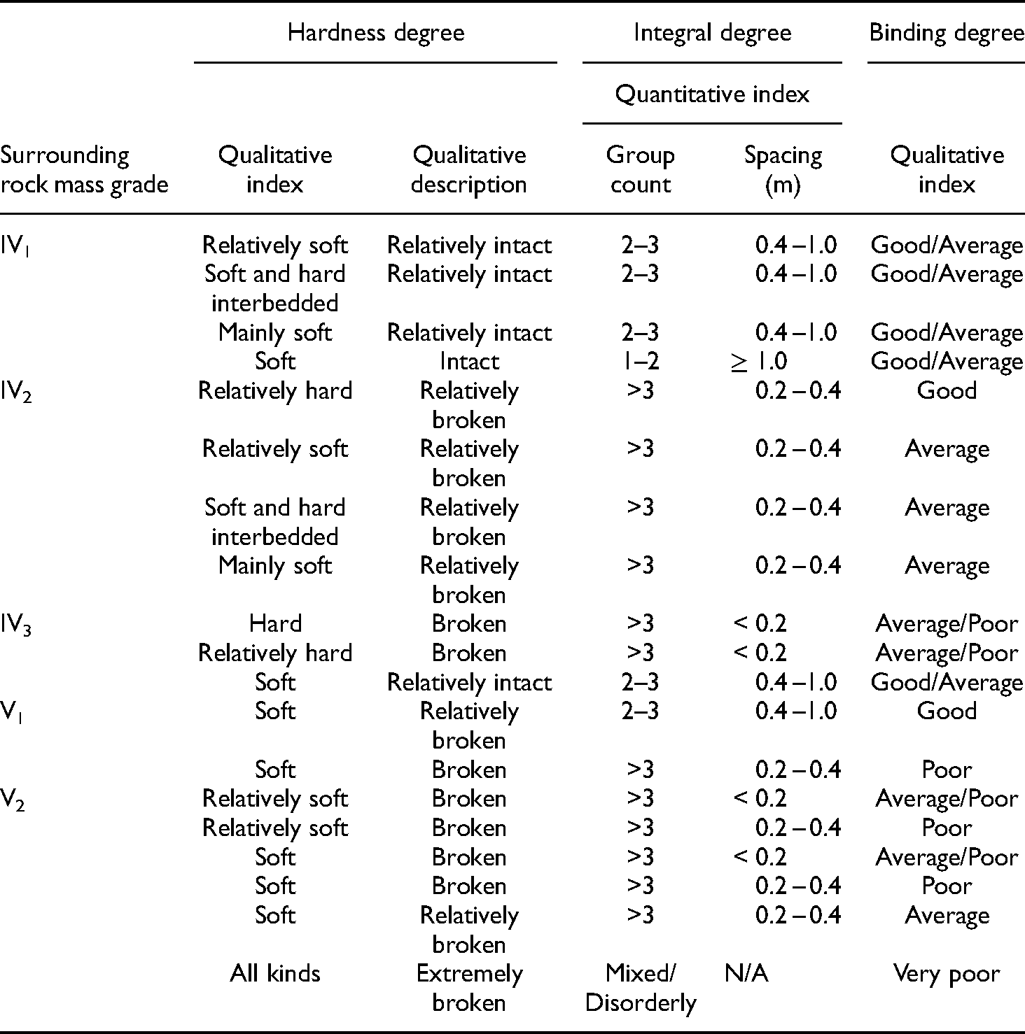
Most published studies of stability problems of jointed rock masses only consider 2 joint sets, e.g., Yeung and Leong,¹⁸ Solak and Schubert,¹⁹ and Delisio et al.²⁰ Based on the Chinese rock mass subclassification system,^21–25 4 independent sets of joints were considered, including 2 sets of inclined joints with different orientations for both soft and hard rock, 1 set of horizontal joints for soft rock, and another set of horizontal joints for hard rock.

Most published studies exploring the stability problems of jointed rock masses have only considered 2 joint sets.^18–20 Based on the Chinese rock mass subclassification system,^21–25 the qualitative description of the subclassification of surrounding rock mass grades IV and V (Table 1) can be obtained, from which the number of joint sets and the range of joint spacing can be determined. In this study, the rock masses were divided into 2 layers, i.e., the upper soft stratum and the lower hard stratum, as shown in Figure 1. For the soft and hard rock strata illustrated in Figure 1, class IV rock including the IV₁, IV₂, IV₃ subclassifications, and class V rock, including the V₁, V₂ sub-classifications, were considered. Six stratum combinations were given as follows: V₁–IV₁, V₂–IV₁, V₁–IV₂, V₂–IV₂, V₁–IV₃, and V₂–IV₃. The properties of the rock strata are listed in Tables 2 and 3.

Figure 1.

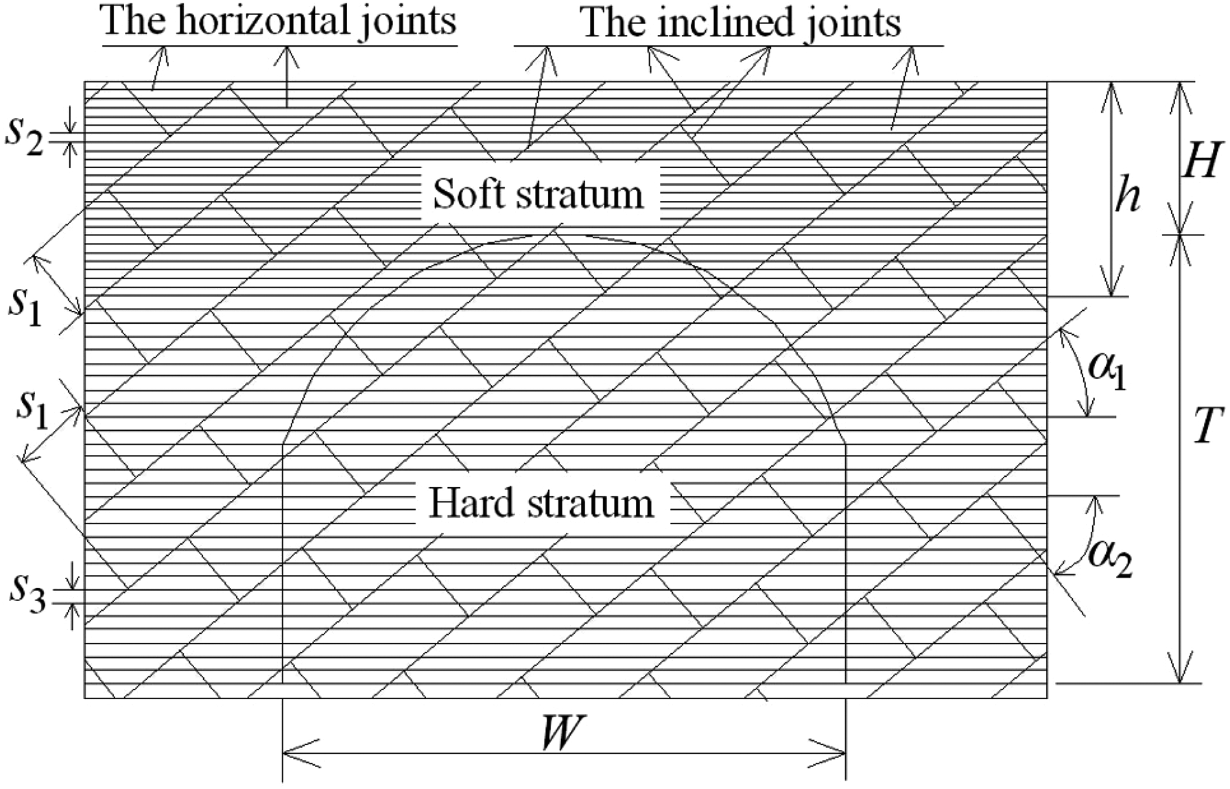
Schematic diagram of joints.

Table 1.

Qualitative subclassification methods for surrounding rock mass grades IV and V.

Surrounding rock mass grade	Hardness degree		Integral degree		Binding degree
	Qualitative index	Qualitative description	Quantitative index		Qualitative index
	Qualitative index	Qualitative description	Group count	Spacing (m)	Qualitative index
IV₁	Relatively soft	Relatively intact	2–3	0.4 –1.0	Good/Average
	Soft and hard interbedded	Relatively intact	2–3	0.4 –1.0	Good/Average
	Mainly soft	Relatively intact	2–3	0.4 –1.0	Good/Average
	Soft	Intact	1–2	≥ 1.0	Good/Average
IV₂	Relatively hard	Relatively broken	>3	0.2 – 0.4	Good
	Relatively soft	Relatively broken	>3	0.2 – 0.4	Average
	Soft and hard interbedded	Relatively broken	>3	0.2 – 0.4	Average
	Mainly soft	Relatively broken	>3	0.2 – 0.4	Average
IV₃	Hard	Broken	>3	< 0.2	Average/Poor
	Relatively hard	Broken	>3	< 0.2	Average/Poor
	Soft	Relatively intact	2–3	0.4 –1.0	Good/Average
V₁	Soft	Relatively broken	2–3	0.4 –1.0	Good
V₁	Soft	Broken	>3	0.2 – 0.4	Poor
V₂	Relatively soft	Broken	>3	< 0.2	Average/Poor
	Relatively soft	Broken	>3	0.2 – 0.4	Poor
	Soft	Broken	>3	< 0.2	Average/Poor
	Soft	Broken	>3	0.2 – 0.4	Poor
	Soft	Relatively broken	>3	0.2 – 0.4	Average
	All kinds	Extremely broken	Mixed/Disorderly	N/A	Very poor

Table 2.

Physical and mechanical parameters of the rock masses and joints.

Stratum	E_e (GPa)	v_e	c_J (kPa)	φ_J (°)
IV₁	4.0–6.0	0.30–0.31	25–40	6–13
IV₂	2.5–4.0	0.31–0.33	10–25	5–11
IV₃	1.3–2.5	0.33–0.35	1–10	4–9
V₁	1.3–2.0	0.35–0.38	0.4–1	2–8
V₂	1.0–1.3	0.38–0.45	0.1–0.4	2–7

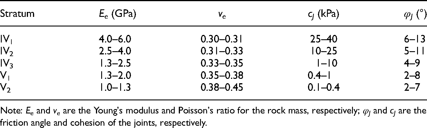
Note: E_e and v_e are the Young's modulus and Poisson's ratio for the rock mass, respectively; φ_J and c_J are the friction angle and cohesion of the joints, respectively.

Table 3.

Physical and mechanical parameters of the rock.

Intact rock material	γ_r (kN/m³)	E_r (GPa)	v_r	φ_r (°)	c_r (MPa)
Regolith	16–23	11–20	0.28–0.40	40.1–48.8	1.0–1.5
Bedrock	23–28	23–30	0.26–0.30	44.0–58.9	1.7–2.0

Note: γ_r, E_r, v_r, φ_r, and c_r, are the density, Young's modulus, Poisson's ratio, friction angle, and cohesion of the intact rock material, respectively.

The ranges of the other factors were determined according to the subclassification system, engineering experiences, field investigations, and observations.^26–32 The span of the tunnel, W, varied from 5–26 m; the height-span ratio of the tunnel, λ, varied from 0.5–2.0; the thickness of the soft overburden, h, ranged from 5–50 m; and the depth of the tunnel, H, varied from 10–100 m. α₁ is the angle of the transfixion inclined joints (10° ≤ α₁ ≤ 80°); α₂ is the angle of the intermittent inclined joints ( − 80° ≤ α₂ ≤ −10°); the lateral pressure coefficient, k, ranged from 0.5–2; s₁ represents the joints spacing of the transfixion inclined joints and the intermittent inclined joints; s₂ denotes the spacing of horizontal joints in the regolith stratum; and s₃ denotes the spacing of horizontal joints in the bedrock stratum. The values of s₁, s₂, and s₃ vary with stratum class, as shown in Table 4.

Table 4.

Range of joint spacing values.

Stratum	s₁ (m)	s₂ (m)	s₃ (m)
IV₁	0.4–1.0	N/A	0.4 – 1.0
IV₂	0.4–1.0	N/A	0.4 – 1.0
IV₃	0.2–0.4	N/A	0.2 – 0.4
V₁	0.2–0.4	0.2–0.4	N/A
V₂	0.2–0.4	0.2–0.4	N/A

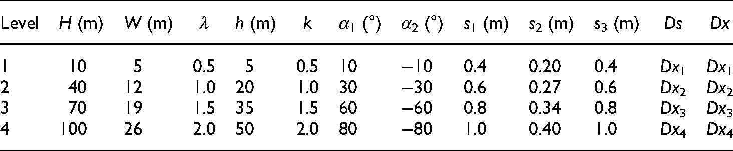
The numerical tests were designed using OATS theory.¹ There were 12 factors: H, W, λ, h, k, α₁, α₂, s_1, s₂, s₃, and the stratum parameters of the upper and lower strata, D_s and D_x, respectively. The range of each factor's value was divided into 4 equal parts, i.e., each factor had 4 levels. It is worth noting that each level of D_s and D_x was treated as a group during the tests, as shown in Tables 5 –7, where Ds₁, Ds₂, Ds₃, and Ds₄ are the 4 levels of the properties of the upper soft stratum; Dx₁, Dx₂, Dx₃, and Dx₄ are the 4 levels of the properties of the lower hard stratum; r₁, φ₁, c₁, E₁, and v₁, denote the density, friction angle, cohesion, elastic modulus, and Poisson's ratio of the upper soft stratum, respectively; r₂, φ₂, c₂, E₂, and v₂ denote the density, friction angle, cohesion, elastic modulus, and Poisson's ratio of the lower hard stratum, respectively; c_J₁ and φ_J₁ represent the joint cohesion and joint friction angle in the upper soft stratum, respectively; and c_J₂ and φ_J₂ represent the joint cohesion and joint friction angle in the hard stratum, respectively. Taking the stratum combination V₁–IV₁ as an example, the range and level of the factors are listed in Table 8. For each stratum combination, 64 test scenarios were determined using the orthogonal array table L₆₄(12¹²);¹ thus, there were 384 test scenarios in total for the 6 stratum combinations.

Table 5.

Physical and mechanical parameters of the rock and joints in the upper soft stratum.

Level	r₁ (kN/m³)		φ₁ (°)		c₁ (MPa)		E₁ (GPa/m)		v ₁		c_J₁ (kPa)		φ_J ₁ (°)
Level	V₁	V₂	V₁	V₂	V₁	V₂	V₁	V₂	V₁	V₂	V₁	V₂	V₁	V₂
Ds ₁	18.5	17.0	22.0	20.0	0.11	0.11	1.30	1.0	0.38	0.45	0.4	0.1	2	2
Ds ₂	19.0	17.5	23.7	20.7	0.14	0.14	1.57	1.1	0.37	0.42	0.6	0.2	4	3
Ds ₃	19.5	18.0	25.4	21.4	0.17	0.17	1.84	1.2	0.36	0.40	0.8	0.3	6	5
Ds ₄	20.0	18.5	27.0	22.0	0.20	0.20	2.10	1.3	0.35	0.38	1	0.4	8	7

Table 6.

Physical and mechanical parameters of the rock in the lower hard stratum.

Level	r₂ (kN/m³)			φ₂ (°)			c₂ (MPa)			E₂ (GPa/m)			v ₂
Level	IV₁	IV₂	IV₃	IV₁	IV₂	IV₃	IV₁	IV₂	IV₃	IV₁	IV₂	IV₃	IV₁	IV₂	IV₃
Dx ₁	22.0	21.0	20.0	34.0	30.0	27	0.50	0.40	0.20	4.00	2.5	1.3	0.3100	0.330	0.350
Dx ₂	22.3	21.3	20.3	35.7	31.3	28	0.57	0.43	0.27	4.83	3.0	1.7	0.3066	0.324	0.344
Dx ₃	22.6	21.6	20.6	37.4	32.6	29	0.64	0.46	0.34	5.66	3.5	2.1	0.3033	0.317	0.337
Dx ₄	23.0	22.0	21.0	39.0	34.0	30	0.70	0.50	0.40	6.50	4.0	2.5	0.3000	0.310	0.330

Table 7.

Physical and mechanical parameters of the joints in the lower hard stratum.

Level	c_J₂ (kPa)			φ_J₂ (°)
Level	IV₁	IV₂	IV₃	IV₁	IV₂	IV₃
Dx ₁	25	10	1	6	5	4
Dx ₂	30	15	4	8	6	5
Dx ₃	35	20	7	10	8	7
Dx ₄	40	25	10	13	11	9

Table 8.

Range and level of the factors for the stratum combination V₁–IV₁.

Level	H (m)	W (m)	λ	h (m)	k	α₁ (°)	α₂ (°)	s₁ (m)	s₂ (m)	s₃ (m)	Ds	Dx
1	10	5	0.5	5	0.5	10	−10	0.4	0.20	0.4	Dx ₁	Dx ₁
2	40	12	1.0	20	1.0	30	−30	0.6	0.27	0.6	Dx ₂	Dx ₂
3	70	19	1.5	35	1.5	60	−60	0.8	0.34	0.8	Dx ₃	Dx ₃
4	100	26	2.0	50	2.0	80	−80	1.0	0.40	1.0	Dx ₄	Dx ₄

Classification of the loosening zone

The collapse area can be obtained after the numerical calculation. Boon et al.³³ examined the collapse patterns of tunnels in complex jointed rock masses consisting of 3 independent sets of joints, and reached the following conclusions: (1) It is possible for all of the joint sets to participate in the collapse mechanism and (2) the collapse mechanisms are numerous. Therefore, it emerges that the prediction of the exact failure location is unlikely to be successful in practice since the collapse location is highly sensitive to the joint patterns and there could be more than one failure mechanism occurring simultaneously. For these reasons, it appears as if the qualitative characterization of collapse failure patterns using specific descriptions is unattainable.

Since the strength and stiffness of rock blocks are large, damage to the surrounding rock is mainly due to the opening and slipping of the joints. Hence, the loosening area can be regarded as the slipping or opening zone. The UDEC can display the slipping and opening zones clearly, as shown in Figure 2. As can be seen in the figure, the slipping zone area is normally larger than the opening zone. Hence, the loosening zone can conservatively be regarded as the slipping zone.

Figure 2.

Loosening zone patterns for tunnels of different depths.

Referring to Figure 2, the loosening zone of the surrounding rock masses can be classified into 3 patterns: the ringent trumpet-shaped loosening zone, the closing-trend trumpet-shaped loosening zone, and the arch-shaped loosening zone. The number of each kind of loosening zone via the 6 stratum combinations is listed in Table 9. This reveals that (1) the number of ringent trumpet-shaped loosening zones decreases with increasing tunnel depth, while contrary to this, the number of arch-shaped loosening zones increases with increasing tunnel depth, and the closing-trend trumpet-shaped loosening zone is the transition state between the other 2 kinds of loosening zone; (2) the number of ringent trumpet-shaped loosening zones is 217 (57 percent of total), and the number of arch-shaped loosening zones is 143 (37 percent of total); (3) the models mostly exhibit ringent trumpet-shaped loosening zones when the depth of the tunnel is less than or equal to 70 m, and models mostly exhibit arch-shaped loosening zones when the tunnel depth is less than or equal to 100 m or greater than 70 m. Therefore, this study focused on the ringent trumpet-shaped and arch-shaped loosening zones.

Table 9.

Number of the 3 types of loosening zones at different depths.

Stratum combination	Ringent trumpet-shaped loosening zone				Closing-trend trumpet-shaped loosening zone				Arch-shaped loosening zone
Stratum combination	10 m	40 m	70 m	100 m	10 m	40 m	70 m	100 m	10 m	40 m	70 m	100 m
V₁–IV₁	14	13	3	0	2	3	3	1	0	0	10	15
V₂–IV₁	16	14	3	0	0	2	2	0	0	0	11	16
V₁–IV₂	16	16	5	0	0	0	4	0	0	0	7	16
V₂–IV₂	16	16	8	0	0	0	1	3	0	0	7	13
V₁–IV₃	15	16	6	0	1	0	2	1	0	0	8	15
V₂–IV₃	16	16	8	0	0	0	1	0	0	0	7	16

Factors influencing the loosening zone

Data envelopment analysis

DEA is a linear programming technique.³ It is a non-parametric method used in the estimation of production functions and has been utilized extensively to estimate measures of technical efficiency in a range of industries.³⁴ Like the stochastic production frontiers, DEA estimates the maximum potential output for a given set of inputs, and has primarily been used in the estimation of efficiency. A key advantage of DEA over previous approaches is that it more easily accommodates both multiple inputs and multiple outputs. Some of the advantages of DEA are: (1) There is no need to explicitly specify a mathematical form for the production function; (2) it has proven to be useful in uncovering relationships that remain hidden from other methodologies; (3) it is capable of handling multiple inputs and outputs; (4) it is capable of being used with any input-output measurement; and (5) the sources of inefficiency can be analysed and quantified for every evaluated unit.

A range of DEA models have been developed that measure efficiency and capacity in different ways. These largely fall into the categories of being either input-oriented or output-oriented models. The CCR model is named after its developers Charnes, Cooper, and Rhodes. This was the first and fundamental DEA model, built on the notion of efficiency as defined by the classical engineering ratio. This model calculates an overall efficiency for the unit in which both its pure technical efficiency and scale efficiency are aggregated into a single value. The obtained efficiency is never absolute as it is always measured relative to the field.

As mentioned in the previous section, based on OAT theory, 384 numerical models were calculated, with 12 influential factors included in each. These influential factors, i.e., the input factors, were controllable; however, the results of the numerical tests—the outputs—such as the area and height of the loosening zone, were uncontrollable. Therefore, in the present study, based on the input-oriented CCR model, the weights of the individual influential factors were analysed.

Quantitative analysis of the weight of each influential factor

For both the ringent trumpet-shaped loosening zone and the arch-shaped boundary, the input factors included H, W, λ, h, k, α₁, α₂, s₁, s₂, s₃, Ds, and Dx. The precise values of each of these factors are listed in Tables 5 –8. As shown in Figure 3, X is defined as the lateral length of the loosening zone on the ground surface; L₁ and L₂ are the widths of the horizontal earth strip above tunnel vault; A₁ and A₂ are the areas of the loosening zone; and V₁ is the height of the loosening zone above the vault of the tunnel. For the ringent trumpet-shaped loosening zone, the outputs were X, L₁, and A₁; for the arch-shaped loosening zone, the outputs were A₂, L_2, V₁, and V₂. The statistical data for X, L₁, A₁, A₂, L_2, V₁, and V₂ are listed in the supplementary material (Tables S1–S3).

Figure 3.

Schematic diagram of model outputs.

The efficiency of each of the influential factors was analysed using MaxDea code; results of this analysis are listed in Tables 10 and 11. These results show that: (1) For the ringent trumpet-shaped loosening zone, the relative degree of influence of the factors was W > H > λ > α₁ > h > Ds > s₁ > k > s₂ > Dx > α₂ > s₃; for the arch-shaped loosening zone, the relative degree of influence was W > λ > H > α₁ > Dx > s₁ > k > s₃ > Ds > s₂ > α₂ > h. This is due to the fact that, with the exception of Dx and Ds, the other 10 factors all share the same value in the 6 stratum combinations; (2) for both types of loosening zone, the span of the tunnel, W, is the most important influential factor. The state of the joints also has significant influence that cannot be neglected in the failure of the loosening zone; (3) for the ringent trumpet-shaped loosening zone, factors such as α₂ and s₃, which are associated with the hard stratum, exert less influence on the failure; correspondingly, for the arch-shaped loosening zone, factors such as α₂ and h, associated with the soft stratum, exert less influence.

Table 10.

Factor weights for the ringent trumpet-shaped loosening zone.

Stratum combination	Weight (%)
Stratum combination	H (m)	W (m)	λ	h (m)	k	α₁ (°)	α₂ (°)	s₁ (m)	s₂ (m)	s₃ (m)	Ds	Dx
V₁–IV₁	13.85	51.74	8.84	3.36	2.81	6.34	1.16	3.09	2.33	1.07	3.32	2.18
V₂–IV₁	12.89	41.01	8.58	9.29	3.63	9.67	0.00	4.89	0.82	0.00	4.89	2.41
V₁–IV₂	13.66	43.72	10.30	7.96	2.87	8.29	0.50	4.19	1.43	0.25	4.31	2.51
V₂–IV₂	9.13	58.98	6.72	3.46	2.93	5.59	1.08	3.22	2.80	0.48	3.24	2.36
V₁–IV₃	10.23	57.35	8.25	5.26	1.28	6.09	0.49	2.70	0.99	0.39	4.30	2.67
V₂–IV₃	13.32	37.18	12.82	6.63	3.70	7.88	1.38	4.14	3.43	0.59	5.87	3.05

Table 11.

Factor weights for the arch-shaped loosening zone.

Stratum combination	Weight (%)
Stratum combination	H (m)	W (m)	λ	h (m)	k	α₁ (°)	α₂ (°)	s₁ (m)	s₂ (m)	s₃ (m)	Ds	Dx
V₁–IV₁	10.53	51.64	11.71	0.00	3.19	7.04	0.34	3.77	2.07	3.06	2.70	3.94
V₂–IV₁	7.46	48.71	9.95	0.53	4.44	6.53	1.06	4.47	2.98	4.03	3.88	5.97
V₁–IV₂	7.94	49.47	10.39	0.00	4.44	6.81	0.10	5.27	2.49	4.01	3.49	5.59
V₂–IV₂	7.79	56.72	9.74	0.00	3.20	5.02	0.48	4.10	2.54	2.88	2.75	4.77
V₁–IV₃	8.12	49.27	9.93	0.14	4.25	7.37	0.58	4.50	2.85	4.00	3.49	5.50
V₂–IV₃	6.78	48.86	16.56	0.00	3.76	5.58	0.43	3.80	2.68	3.19	2.95	5.29

Prediction of loosening zone boundaries

It is well known that the range of the loosening zone has a significant impact on the construction safety and support of tunnels; hence it is of great importance to derive a formula for the loosening zone boundary, from which the loosening zone range can be defined. The previous section analysed the influential factors of the loosening zone, revealing that different stratum combinations have different factor weights. In this study, the factors with weights greater than 2% were considered to be important parameters that could not be ignored. On this basis, the one-dimensional nonlinear and multiple linear regression models were constructed, and the prediction formulae of the boundaries of the ringent trumpet-shaped and arch-shaped loosening zones were deduced. The first step was to identify the functions for the 2 types of loosening zone boundaries.

The functions of the loosening zone boundaries

Curve fitting is one of the most powerful and most widely used analytical tools in Origin code. Origin code provides tools for linear and nonlinear curve fitting, along with validation and goodness-of-fit tests. Let the expression y = f(x) indicate any element belonging to the set of curves which define a possible range of the loosening zone in the Cartesian reference frame x-y.

For the ringent trumpet-shaped loosening zone exhibited by 217 models, the right bottom corner of the tunnel is used as the origin of coordinate system, as shown in Figure 4.

Figure 4.

Schematic diagram of models with ringent trumpet-shaped loosening zones.

The right boundary of the ringent trumpet-shaped loosening zone shown in Figure 4 can be simulated by 2 functions, the power function (y = ax^b) and the parabolic function (y = a + bx + cx²). For each test, the undetermined coefficients, i.e., a and b in the power function and a, b, and c in the parabolic function, can be determined with regression tools by utilizing Origin code. As examples, the boundaries of loosening zones from numerical tests No. 8, No. 20, No. 28, and No. 35 are shown in Figure 5; regression results are listed in Table 12. Due to its higher coefficient and lower number of parameters, the power function was chosen as the boundary function of the ringent trumpet-shaped loosening zone in this study.

Figure 5.

Fitting comparison of the power function and the parabolic equation.

Table 12.

Fitting results for the power function and parabolic equation.

Model number	Fitting results
Model number	y = f (x)	a	b	c	σ_a	σ_b	σ_c	R
8	y = ax^b	0.0003	3.9795	N/A	0.0005	0.5329	N/A	0.9599
8	y = a + bx + cx²	2.4825	−1.4649	0.1748	3.3635	0.8216	0.0418	0.9207
20	y = ax^b	0.0002	6.0959	N/A	0.0005	0.8051	N/A	0.9656
20	y = a + bx + cx²	3.0683	−2.0959	0.1622	6.3278	1.1815	0.0452	0.8819
28	y = ax^b	0.0023	3.6186	N/A	0.0032	0.5226	N/A	0.9588
28	y = a + bx + cx²	2.4423	−2.0595	0.3088	4.4528	1.1694	0.0669	0.9359
35	y = ax^b	0.0001	6.1570	N/A	0.0001	0.7114	N/A	0.9761
35	y = a + bx + cx²	6.8332	−2.2421	0.1012	0.1469	1.1622	0.0271	0.8822

Note: a, b, and c are the values of the coefficients; σ_a, σ_b, and σ_c are the standard errors of the coefficients; R is the correlation coefficient of the equations.

Similarly, for the 143 models with the arch-shaped loosening zone, as shown in Figure 6, the expression of the boundary can be simulated by 3 functions: the inversely proportional function (y = 1/[a + bx]), the power function (y = a + bx^c), and the parabolic function (y = a + bx + cx²). The boundaries of the loosening zones from numerical tests No. 22, No. 21, No. 53, and No. 59 are shown in Figure 7; regression results are listed in Table 13. Due to its higher coefficient and lower number of parameters, the inversely proportional function was chosen as the boundary function of the ringent trumpet-shaped loosening zone in this study.

Figure 6.

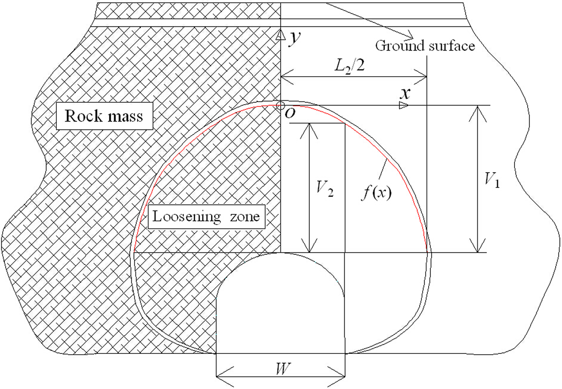
Schematic diagram of models with arch-shaped loosening zones.

Figure 7.

Fitting comparison of the inversely proportional function, the power function, and the parabolic equation.

Table 13.

Fitting results for the inversely proportional function, power function, and parabolic equation.

Model number	Fitting results
Model number	y = f (x)	a	b	c	σ_a	σ_b	σ_c	R
22	y = 1/ (a + bx)	−0.1959	0.0061	N/A	0.0399	0.0014	N/A	0.9973
	y = a + bx^c	−2.2311	0.0006	3.2678	1.1028	0.0008	0.3869	0.9616
	y = a + bx + cx²	−1.2279	0.5255	−0.0643	1.8390	0.3319	0.0113	0.9376
51	y = 1/ (a + bx)	−0.9089	0.1569	N/A	0.1567	0.0319	N/A	0.9926
	y = a + bx^c	−1.2027	0.0147	3.7830	0.2625	0.0127	0.5275	0.9506
	y = a + bx + cx²	−0.2259	0.2185	−0.3241	0.5707	0.5255	0.0992	0.9398
53	y = 1/ (a + bx)	−1.3558	0.1866	N/A	0.4275	0.0716	N/A	0.9968
	y = a + bx^c	−0.5834	−0.0108	3.2472	0.1455	0.0057	0.2698	0.9457
	y = a + bx + cx²	−0.2604	0.2937	−0.1647	0.3710	0.2709	0.0379	0.9318
59	y = 1/ (a + bx)	−0.2712	0.0101	N/A	0.0676	0.0029	N/A	0.9969
	y = a + bx^c	−3.2198	−0.0005	3.4305	1.0838	0.0006	0.3689	0.9648
	y = a + bx + cx²	−0.8716	0.4689	−0.0715	2.3251	0.4074	0.0146	0.9358

Note: a, b, and c are the values of the coefficients; σ_a, σ_b, and σ_c are the standard errors of the coefficients; R is the correlation coefficient of the equations.

Prediction formulae of the loosening zone boundaries

Prediction formulae of typical geometric quantities

For the 217 models with the ringent trumpet-shaped loosening zone, according to Tables 5 –8, one-dimensional nonlinear regression models of X (the lateral length of the loosening zone on the ground surface) and L₁ (the width of the horizontal strip of earth above the tunnel vault) can be established using the least squares method. As an example, for the V₁–IV₁ stratum combination, the one-dimensional nonlinear regression formulae of X are listed in Table 14, where 10 m ≤ H ≤ 40 m; 5 m ≤ W ≤ 26 m; 0.5 ≤ λ ≤ 2; 5 m ≤ h ≤ 50 m; 0.5 ≤ k ≤ 2; and 10° ≤ α₁ ≤ 80°. For the stratum combinations V₁–IV₁, V₁–IV₂, and V₁–IV₃, the range of s₁ is 0.4 m ≤ s₁ ≤ 1.0 m; for the stratum combinations V₂–IV₁, V₂–IV₂, and V₂–IV₃, the range of s₂ is 0.2 m ≤ s₂ ≤ 0.4 m. When the values of the stratum parameters are approximate to Ds₁ (see Table 5), then Ds takes the value 1; analogously, Ds and Dx can take the values 1, 2, 3, or 4, corresponding to different stratum parameters. Statistically speaking, the values of the correlation coefficient, R, are all greater than 0.900, indicating that all of the empirical formulae are correct.

Table 14.

One-dimensional nonlinear regression formulae of X for the stratum combination V₁–IV ₁ .

Factor	Nonlinear regression formula	R
H	X = 58.543 × 1.005 ^H	0.998
W	X = 0.572 W + 61.683	0.993
λ	X = −22.086λ² + 109.281λ − 34.428	0.995
h	X = 0.493 h + 42.199	0.971
k	X = 55.509e^0.222k	0.958
α ₁	X = −6.095tan²α₁ − 31.647tanα₁ + 37.461	0.934
s ₁	X = −15.136 s₁² − 5.980s₁ + 66.011	0.952
s ₂	X = −40.059s₂² − 87.22s₂ + 90.320	0.938
Ds	X = −6.646 Ds + 88.904	0.947
Dx	X = −2.850Dx + 60.68	0.947

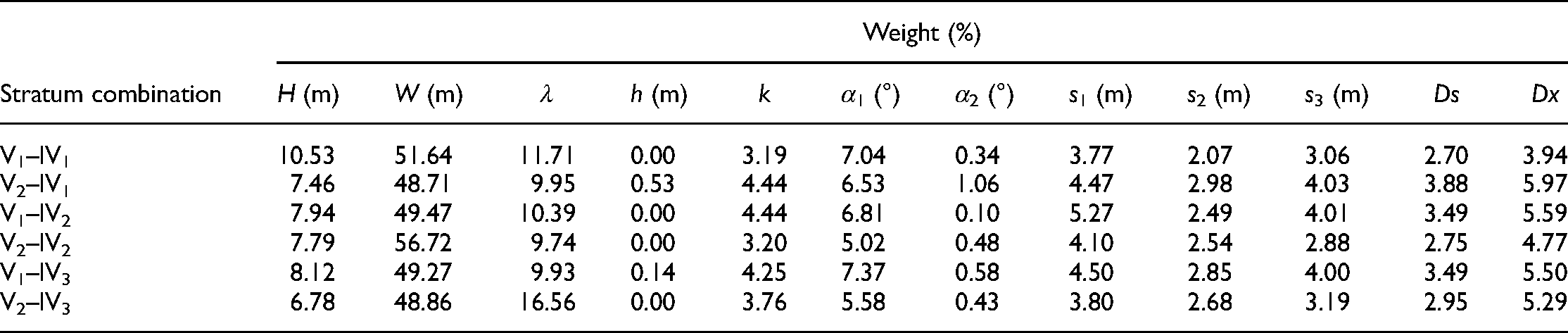
Suppose X and 1.005 ^H , W, λ², λ, h, e^0.222k, tan²α₁, tanα₁, s₁², s₁, s₂², s₂, Ds, and Dx have a linear relationship. Through the construction of multiple linear regression models, the value of each undetermined coefficient can be calculated using the least squares method and the calculation formula of X obtained: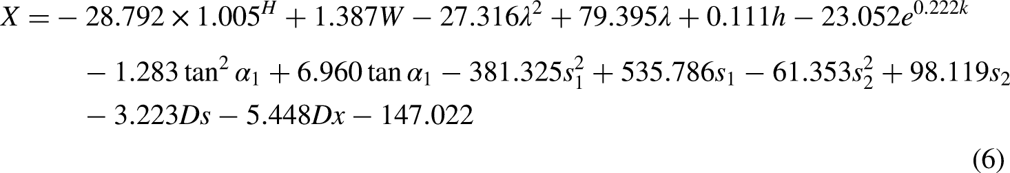

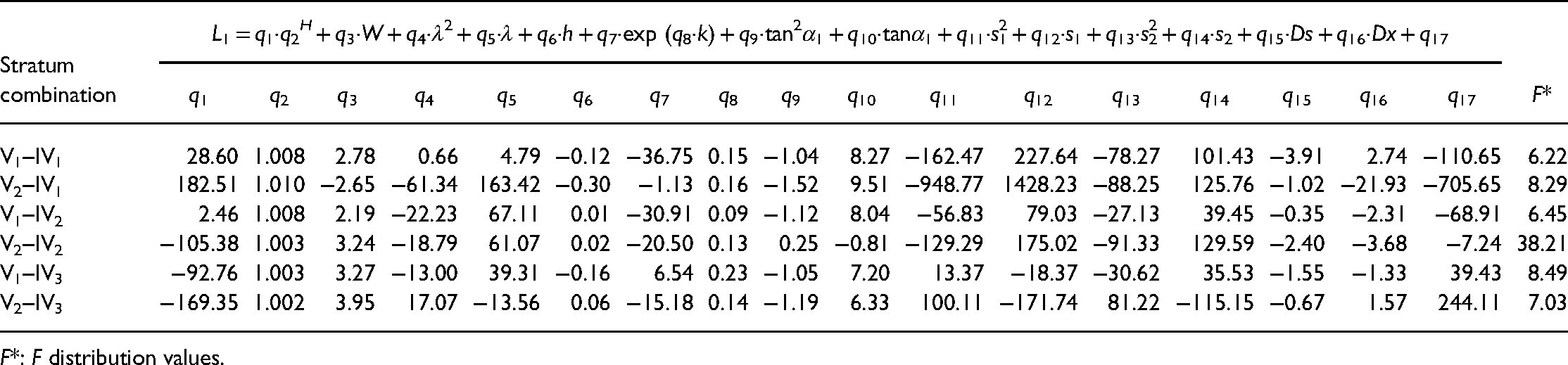
\begin{aligned} X = & - 28.792 \times {1.005}^{H} + 1.387 W - 27.316 λ^{2} + 79.395 λ + 0.111 h - 23.052 e^{0.222 k} \\ - 1.283 \tan^{2} α_{1} + 6.960 \tan α_{1} - 381.325 s_{1}^{2} + 535.786 s_{1} - 61.353 s_{2}^{2} + 98.119 s_{2} \\ - 3.223 D s - 5.448 D x - 147.022 \end{aligned}

(6)

The analysis of variance, popularly known as ANOVA, can be used to verify the rationality of the above equation. The variance analysis is listed in the supplementary material (Table S4). For Eq. (6), the degree of freedom of distribution F(14, 12) = 5.835. For 0.005, 0.01, 0.025, 0.05, and 0.1 significance levels, F* = 5.835 > F_0.005(14, 12) = 4.43 > F_0.01(14, 12) = 3.80 > F_0.025(14, 12) = 3.05 > F_0.05(14, 12) = 2.53 > F_0.1(14, 12) = 2.05. Thus, it can be seen that the regression was reasonable.

For other stratum combinations, the multiple linear regression equations of X and L₁ are listed in Tables 15 and 16. Similarly, the multiple linear regression equations of L₂, V₁, and V₂ can be obtained (Tables 17 –19). The F distribution values of these equations are listed in Tables 15 –19; the rationality of the above equations was also verified using ANOVA.

Table 15.

Multiple linear regression equations of X.

Stratum combination	X = p₁·p₂ ^H + p₃·W + p₄·λ² + p₅·λ + p₆·h + p₇·exp (p₈·k) + p₉·tan²α₁ + p₁₀·tanα₁ + p₁₁·s₁² + p₁₂·s₁ + p₁₃·s₂² + p₁₄·s₂ + p₁₅·Ds + p₁₆·Dx + p₁₇																	F*
Stratum combination	p ₁	p ₂	p ₃	p ₄	p ₅	p ₆	p ₇	p ₈	p ₉	p ₁₀	p ₁₁	p ₁₂	p ₁₃	p ₁₄	p ₁₅	p ₁₆	p ₁₇	F*
V₁–IV₁	−28.79	1.005	1.39	−27.32	79.40	0.11	−23.05	0.22	−1.28	6.96	−381.33	535.79	−61.35	98.12	−3.22	−5.45	−177.02	5.84
V₂–IV₁	−105.47	1.006	−2.34	−55.53	151.04	−0.76	3.77	0.18	−0.84	7.65	−897.79	1329.57	−90.96	127.63	−2.72	−15.54	−579.71	6.52
V₁–IV₂	11.81	1.010	2.15	−14.73	40.77	−0.05	−25.74	0.17	−0.61	5.90	−71.38	106.01	−99.03	142.10	−0.09	−1.89	−98.86	6.39
V₂–IV₂	−40.98	1.002	2.99	−12.15	36.45	0.08	−48.19	0.13	0.71	−3.49	−251.26	357.98	−122.08	169.76	−0.94	−3.70	−91.31	29.73
V₁–IV₃	−42.03	1.001	2.96	−2.89	13.49	−0.12	6.60	0.18	0.08	0.62	−86.41	131.01	1.51	−4.80	−0.12	−2.21	33.31	13.73
V₂–IV₃	−2.05	1.002	4.00	22.64	−36.00	−0.10	−15.48	0.08	−0.90	5.82	63.09	−121.28	98.54	−130.49	−0.72	3.11	81.96	7.25

F*: F distribution values.

Table 16.

Multiple linear regression equations of L ₁ .

Stratum combination	L₁ = q₁·q₂ ^H + q₃·W + q₄·λ² + q₅·λ + q₆·h + q₇·exp (q₈·k) + q₉·tan²α₁ + q₁₀·tanα₁ + q₁₁·s₁² + q₁₂·s₁ + q₁₃·s₂² + q₁₄·s₂ + q₁₅·Ds + q₁₆·Dx + q₁₇																	F*
Stratum combination	q ₁	q ₂	q ₃	q ₄	q ₅	q ₆	q ₇	q ₈	q ₉	q ₁₀	q ₁₁	q ₁₂	q ₁₃	q ₁₄	q ₁₅	q ₁₆	q ₁₇	F*
V₁–IV₁	28.60	1.008	2.78	0.66	4.79	−0.12	−36.75	0.15	−1.04	8.27	−162.47	227.64	−78.27	101.43	−3.91	2.74	−110.65	6.22
V₂–IV₁	182.51	1.010	−2.65	−61.34	163.42	−0.30	−1.13	0.16	−1.52	9.51	−948.77	1428.23	−88.25	125.76	−1.02	−21.93	−705.65	8.29
V₁–IV₂	2.46	1.008	2.19	−22.23	67.11	0.01	−30.91	0.09	−1.12	8.04	−56.83	79.03	−27.13	39.45	−0.35	−2.31	−68.91	6.45
V₂–IV₂	−105.38	1.003	3.24	−18.79	61.07	0.02	−20.50	0.13	0.25	−0.81	−129.29	175.02	−91.33	129.59	−2.40	−3.68	−7.24	38.21
V₁–IV₃	−92.76	1.003	3.27	−13.00	39.31	−0.16	6.54	0.23	−1.05	7.20	13.37	−18.37	−30.62	35.53	−1.55	−1.33	39.43	8.49
V₂–IV₃	−169.35	1.002	3.95	17.07	−13.56	0.06	−15.18	0.14	−1.19	6.33	100.11	−171.74	81.22	−115.15	−0.67	1.57	244.11	7.03

F*: F distribution values.

Table 17.

Multiple linear regression equations of L ₂ .

Stratum combination	L₂ = b₁·b₂ ^H + b₃·W + b₄·λ² + b₅·λ + b₆·exp (b₇·k) + b₈·tan²α₁ + b₉·tanα₁ + b₁₀·s₁² + b₁₁·s₁ + b₁₂·s₂² + b₁₃·s₂ + b₁₄·s₃² + b₁₅·s₃ + b₁₆·Ds + b₁₇·Dx + b₁₈																		F*
Stratum combination	b ₁	b ₂	b ₃	b ₄	b ₅	b ₆	b ₇	b ₈	b ₉	b ₁₀	b ₁₁	b ₁₂	b ₁₃	b ₁₄	b ₁₅	b ₁₆	b ₁₇	b ₁₈	F*
V₁–IV₁	26.03	0.92	1.78	0.63	4.22	−32.71	0.10	−0.94	6.78	−151.10	198.05	−76.70	91.29	−372.099	538.032	−3.40	2.49	−69.34	5.87
V₂–IV₁	158.78	0.81	−1.56	−57.05	138.91	−0.98	0.11	−1.37	7.80	−929.79	1228.28	−84.72	108.15	−83.0557	118.7424	−0.89	−19.96	−393.10	7.21
V₁–IV₂	2.12	0.95	1.91	−21.56	48.99	−26.58	0.05	−1.01	6.59	−53.42	67.18	−25.50	33.14	59.5686	−13.5936	−0.30	−2.10	−48.40	6.31
V₂–IV₂	−72.71	0.96	1.91	−16.16	47.02	−18.04	0.09	0.23	−0.66	−117.65	159.27	−85.85	114.04	314.5779	−453.629	−2.09	−3.35	−6.41	15.42
V₁–IV₃	−91.83	0.88	2.91	−10.92	25.94	5.95	0.13	−0.95	5.90	12.03	−16.90	−29.40	30.91	−24.5245	41.6064	−1.35	−1.21	15.64	8.19
V₂–IV₃	−155.80	0.84	3.12	12.97	−11.53	−14.12	0.13	−1.07	5.19	88.10	−159.72	78.78	−97.88	22.9775	−36.624	−0.58	1.43	123.18	6.38

F*: F distribution values.

Table 18.

Multiple linear regression equations of V ₁ .

Stratum combination	V₁ = j₁·ln (H + j₂) + j₃·W + j₄·λ² + j₅·λ + j₆·k^j₇ + j₈/(j₉·tan²α₁ + j₁₀·tanα₁ + j₁₁) + j₁₂·s₁² + j₁₃·s₂² + j₁₄·s₂ + j₁₅·s₃² + j₁₆·s₃ + j₁₇·Ds + j₁₈·Dx + j₁₉																			F*
Stratum combination	j ₁	j ₂	j ₃	j ₄	j ₅	j ₆	j ₇	j ₈	j ₉	j ₁₀	j ₁₁	j ₁₂	j ₁₃	j ₁₄	j ₁₅	j ₁₆	j ₁₇	j ₁₈	j ₁₉	F*
V₁–IV₁	30.18	−36.62	3.05	−37.56	80.44	5.41	0.30	−0.19	0.003	−0.012	0.029	−50.47	−318.37	439.84	−408.90	560.45	4.71	−19.84	−187.57	10.75
V₂–IV₁	1.74	−51.11	1.75	−8.94	26.23	20.27	0.14	−0.52	0.003	−0.015	0.037	−22.15	−74.22	93.42	−91.27	123.69	3.05	−6.12	−93.45	13.39
V₁–IV₂	−1.13	−67.37	4.03	−4.18	2.18	−2.18	0.14	−2.73	0.002	−0.006	0.022	−0.46	−4.78	−41.35	65.46	−14.16	−4.68	0.50	−34.49	20.80
V₂–IV₂	2.45	−64.87	3.16	23.73	−52.74	−6.68	0.36	−0.07	0.003	−0.013	0.025	75.48	410.65	−571.40	345.69	−472.53	−1.99	16.95	−301.78	8.23
V₁–IV₃	3.28	−62.61	2.43	−1.63	0.00	−3.54	0.18	−0.26	0.003	−0.014	0.031	6.76	−3.76	11.66	−26.95	43.34	−1.01	−0.90	39.07	10.56
V₂–IV₃	−0.50	−55.35	1.16	1.23	0.00	−9.20	0.37	−0.27	0.003	−0.009	0.021	−14.81	24.54	−18.99	25.25	−38.15	0.06	−0.72	77.20	7.72

F*: F distribution values.

Table 19.

Multiple linear regression equations of V ₂ .

Stratum combination	V₂ = l₁·ln (H + l₂) + l₃·W + l₄·λ² + l₅·λ + l₆·k^l₇ + l₈/(l₉·tan²α₁ + l₁₀·tanα₁ + l₁₁) + l₁₂·s₁² + l₁₃·s₂² + l₁₄·s₂ + l₁₅·s₃² + l₁₆·s₃ + l₁₇·Ds + l₁₈·Dx + l₁₉																			F*
Stratum combination	l ₁	l ₂	l ₃	l ₄	l ₅	l ₆	l ₇	l ₈	l ₉	l ₁₀	l ₁₁	l ₁₂	l ₁₃	l ₁₄	l ₁₅	l ₁₆	l ₁₇	l ₁₈	l ₁₉	F*
V₁–IV₁	2.47	−64.30	2.21	38.78	−92.35	−3.01	0.30	−0.34	0.003	−0.016	0.033	27.79	64.25	−65.48	123.14	−206.53	−0.55	6.96	92.41	7.26
V₂–IV₁	93.51	−62.51	0.79	1.37	−17.36	45.50	0.08	−0.41	0.005	−0.024	0.049	−36.74	−102.20	129.45	−95.58	132.76	3.50	−8.40	−123.51	10.00
V₁–IV₂	0.31	−66.55	2.17	27.07	−69.89	−5.46	0.13	−1.00	0.001	−0.006	0.025	6.92	−30.78	63.94	36.23	−87.57	−0.82	0.42	79.63	13.33
V₂–IV₂	2.48	−66.17	1.89	20.33	−47.38	2.10	0.26	−0.24	0.003	−0.013	0.029	45.21	224.36	−293.55	194.56	−276.27	−1.55	12.02	121.39	6.77
V₁–IV₃	−0.50	−66.22	1.16	1.23	0.00	−9.20	0.16	−0.27	0.003	−0.012	0.032	−14.81	24.54	−18.99	25.25	−38.15	0.06	−0.72	17.20	7.72
V₂–IV₃	−6.61	−64.86	1.26	−26.77	41.38	−68.79	0.27	−0.14	0.002	−0.029	0.213	−103.88	114.46	−159.34	51.21	−56.96	2.56	−22.22	251.18	11.21

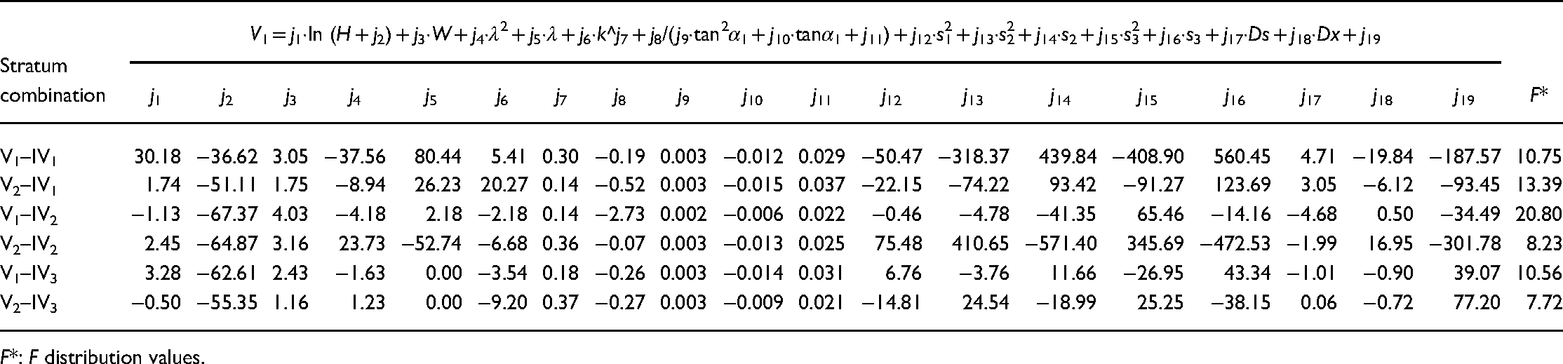
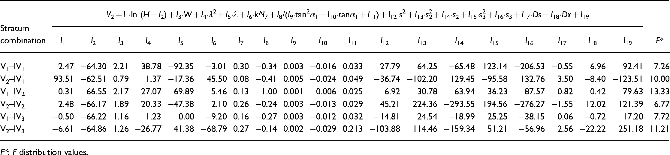
F*: F distribution values.

Prediction formulae

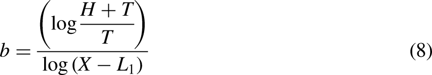
In the case of the ringent trumpet-shaped loosening zone shown in Figure 4, the boundary function of the loosening zone was considered to be y = ax^b. Once the prediction formulae of X and L₁ had been derived, the coefficients, a and b, could be calculated:

a = T {(\frac{L_{1} - W}{2})}^{- b}

(7)

b = \frac{(\log \frac{H + T}{T})}{\log (X - L_{1})}

(8)

By virtue of Eqs. (7) and (8), the expression of the boundary could be obtained. Following a similar procedure, the parameters involved in the boundary function of arch-shaped loosening zone, expressed as y = 1/(a + bx), could be calculated:

a = \frac{V_{1} W - V_{1} L_{2} - V_{2} W}{(V_{1} - V_{2}) (W - L_{2}) V_{1}}

(9)

b = \frac{2 V_{2}}{(V_{1} - V_{2}) (W - L_{2}) V_{1}}

(10)

Calculation formulae for loosening pressures

Once the boundary of the loosening zone was obtained, the force field could be determined using the principle of stress transformation. Let r₁ represent the density of the soft stratum, c_J₁ denote the joint cohesion of the soft stratum, φ_J₁ represent the joint internal friction angle of the soft stratum, r₂ represent the density of the hard stratum, c_J₂ denote the joint cohesion of the hard stratum, φ_J₂ represent the joint internal friction angle of the hard stratum, h denote the depth of the soft stratum, H denote the depth of the tunnel, and W represent the span of the tunnel. The analytical formulae of the loosening pressures were deduced for the following 2 conditions: (1) embedded depth deeper than the soft layer (H > h); (2) embedded depth shallower than the soft layer (H ≤ h).

Condition 1: The embedded depth is deeper than the soft layer (H > h)

Loosening pressures of models with ringent trumpet-shaped loosening zones

As shown in Figures 8 and 9, the straight line, M₁N₁, denotes the interface between the soft and hard strata, which divides the loosening zone above the tunnel vault into 2 parts: the geometric regions E₁M₁N₁B₁ and M₁R₁K₁N₁.

Figure 8.

Calculation model (No. 1).

Figure 9.

Calculation model (No. 2).

The geometric region D₁U₁V₁C₁ denotes the differential stratum strip. Force field analyses were carried out; details of the derivation of the support pressures are illustrated in Appendix 1. The computational formulae of the vertical pressure of the tunnel, q, could then be obtained:

\begin{aligned} q = & λ_{2} \cdot 2^{(k_{2} \tan φ_{J 2} - 1)} \cdot (2 h + 2 (H - h) + X \tan ε)^{(1 - k_{2} \tan φ_{J 2})} \\ + \frac{h γ_{2} (2 - k_{2} \tan φ_{J 2}) + X γ_{2} \tan ε (1 + k_{2} \tan φ_{J 2})}{2 k_{2} \tan φ_{J 2}^{(k_{2} \tan φ_{J 2} - 1)}} \\ - \frac{c_{J 2}}{k_{2} \tan φ_{J 2} - 1} - \frac{(H - h) γ_{2}}{k_{2} \tan φ_{J 2}} \end{aligned}

(11)

\begin{aligned} λ_{2} & = \frac{q_{0}}{2^{(k_{2} \tan φ_{J 2} - 1)}} + \frac{2 c_{J 2} k_{2} \tan φ_{J 2} {(2 h + X \tan ε)}^{(k_{2} \tan φ_{J 2} - 1)}}{2^{(k_{2} \tan φ_{J 2} - 1)} k_{2} \tan φ_{J 2} (k_{2} \tan φ_{J 2} - 1)} \\ - \frac{h γ_{2} (2 - k_{2} \tan φ_{J 2}) {(2 h + X \tan ε)}^{(k_{2} \tan φ_{J 2} - 1)}}{2^{(k_{2} \tan φ_{J 2} - 1)} k_{2} \tan φ_{J 2} (k_{2} \tan φ_{J 2} - 1)} \\ + \frac{X γ_{2} \tan ε (1 + k_{2} \tan φ_{J 2}) {(2 h + X \tan ε)}^{(k_{2} \tan φ_{J 2} - 1)}}{2^{(k_{2} \tan φ_{J 2} - 1)} k_{2} \tan φ_{J 2} (k_{2} \tan φ_{J 2} - 1)} \end{aligned}

(12)

For the calculation of the lateral pressure, according to traditional approaches such as Terzaghi theory,³⁵ the calculation formulae are given on the basis of Rankine's ratio.

However, it is well known that Rankine's ratio (the active earth pressure coefficient) is applied to earth pressure with the conditions: (1) The smooth surface which is the interface between the wall and soil is frictionless; (2) the supported soil is homogeneous and isotropic. In addition, when the critical slip planes are oriented at 45° ± φ/2, the active Rankine's ratio is k_a = tan²(45°-φ/2). Krynine,³⁶ Ladanyi and Hoyaux,³⁷ and Handy³⁸ found that since k_a was derived from the assumption that the horizontal and vertical stresses are the principal stresses, using k_a is only valid when there is no friction (shear stress) between the till material and the sides of the ditch. However, Terzaghi theory posits that friction exists at the sides of the ditch. Therefore, the active Rankine's ratio, k_a, cannot be used. Wang and Zhu³⁹ also verified this perspective.

In order to avoid the unrealistic assumption of Rankine's active earth pressure, the slip angle is corrected using the following formula (referring to Figure 8):

\tan β = \frac{L_{1} - W}{2 T}

(13)

On this basis, the lateral pressure can be written as

e_{1} = q \tan^{2} β = q {(\frac{L_{1} - W}{2 T})}^{2}

(14)

e_{2} = e_{1} + γ_{2} T \tan^{2} β = e_{1} + γ_{2} T {(\frac{L_{1} - W}{2 T})}^{2}

(15)

Loosening pressures of models with arch-shaped loosening zones

As is shown in Figures 10 and 11, the straight line, M₂N₂, denotes the interface of the soft and hard strata, while the geometric region, D₃U₃V₃C₃, denotes the differential stratum strip. Force field analyses were carried out; details of the derivation of the support pressures are illustrated in Appendix 2.

Figure 10.

Calculation model (No. 3).

Figure 11.

Calculation model (No. 4).

The vertical force, q*, can be written as

q^{*} = λ_{4} (V_{1} - H)^{(k_{2} \tan φ_{J 2} + 1)} - \frac{2 c_{J 2} (k_{2} \tan φ_{J 2} - 1) + a γ_{2} (k_{2} \tan φ_{J 2} + 1) {(V_{1} - H)}^{2}}{2 [{(k_{2} \tan φ_{J 2})}^{2} - 1]}

(16)

\begin{aligned} λ_{4} = & \frac{2 q_{0}^{*} [{(k_{2} \tan φ_{J 2})}^{2} - 1] + 2 c_{J 2} (k_{2} \tan φ_{J 2} - 1) + a γ_{2} {(H - h - V_{1})}^{2}}{2 [{(k_{2} \tan φ_{J 2})}^{2} - 1] {(H - h - V_{1})}^{(k_{2} \tan φ_{J 2} + 1)}} \\ + \frac{a γ_{2} (k_{2} \tan φ_{J 2} + 1) {(H - h - V_{1})}^{2}}{2 [{(k_{2} \tan φ_{J 2})}^{2} - 1] {(H - h - V_{1})}^{(k_{2} \tan φ_{J 2} + 1)}} \end{aligned}

(17)

The lateral pressure can be written as

e_{1}^{*} = q^{*} \tan^{2} β = q^{*} {(\frac{L_{2} - W}{2 T})}^{2}

(18)

e_{2}^{*} = e_{1}^{*} + T γ_{2} \tan^{2} β = e_{1}^{*} + T γ_{2} {(\frac{L_{2} - W}{2 T})}^{2}

(19)

Condition 2: The embedded depth is shallower than the soft layer (H < h)

Loosening pressures of models with ringent trumpet-shaped loosening zones

As shown in Figure 12, when h ≥ H, the tunnels are in homogeneous rock masses. The derivation procedure for q is the same as that used for q₀, which was described in section 4.1.1. The calculation formulae of the loosening pressure can be directly written as:

\begin{aligned} q = & λ_{5} \cdot 2^{(1 - k_{1} \tan φ_{J 1})} \cdot (2 H - X \tan ε)^{(k_{1} \tan φ_{J 1} - 1)} \\ + \frac{2 X \tan ε (X γ_{1} \tan ε - 4 c_{J 1} - X k_{1} γ_{1} \tan ε \tan ε)}{(2 H - X \tan ε) (4 k_{1}^{2} ta n^{2} φ_{J 1} - 24 k_{1} \tan φ_{J 1} + 16)} \\ + \frac{8 h^{2} (2 c_{J 1} - c_{J 1} k_{1} \tan φ_{J 1} - γ_{1} X \tan ε + 2 X c_{J 1} k_{1} \tan φ_{J 1} \tan ε)}{(2 H - X \tan ε) (4 k_{1}^{2} ta n^{2} φ_{J 1} - 24 k_{1} \tan φ_{J 1} + 16)} \\ + \frac{8 H^{2} γ_{1} (1 - k_{1} \tan φ_{J 1})}{(2 H - X \tan ε) (4 k_{1}^{2} ta n^{2} φ_{J 1} - 24 k_{1} \tan φ_{J 1} + 16)} \end{aligned}

(20)

λ_{5} = \frac{2^{(1 - k_{1} \tan φ_{J 1})} (X \tan ε) (X γ_{1} \tan ε - 4 c_{J 1} - X k_{1} γ_{1} \tan ε \tan ε)}{(4 k_{1}^{2} ta n^{2} φ_{J 1} - 24 k_{1} \tan φ_{J 1} + 16) {(- X \tan ε)}^{(k_{1} \tan φ_{J 1} - 1)}}

(21)

e_{1} = q \tan^{2} β = q {(\frac{L_{1} - W}{2 T})}^{2}

(22)

e_{2} = e_{1} + [(h - H) γ_{1} + (T + H - h) γ_{2}] {(\frac{L_{1} - W}{2 T})}^{2}

(23)

Figure 12.

Calculation model (No. 5).

Loosening pressures of models with arch-shaped loosening zones

As shown in Figure 13, when h ≥ H, the tunnels are in homogeneous rock masses. The derivation procedure for q^* is the same as that used for q₀*, which was described in section 4.1.2. The calculation formulae of the loosening pressures can be directly written as:

q^{*} = λ_{6} (V_{1} - H)^{(k_{1} \tan φ_{J 1} + 1)} - \frac{2 c_{J 1} (k_{1} \tan φ_{J 1} - 1) + a γ_{1} {(V_{1} - H)}^{2} (1 + k_{1} \tan φ_{J 1})}{2 [{(k_{1} \tan φ_{J 1})}^{2} - 1]}

(24)

λ_{6} = a^{(k_{1} \tan φ_{J 1} + 1)} [μ γ_{1} (H - V_{1}) + c_{J 1} k_{1} \tan φ_{J 1} - c_{J 1}] + \frac{γ_{1} (k_{1} \tan φ_{J 1} + 1) + a^{k_{1} \tan φ_{J 1}}}{2}

(25)

e_{1}^{*} = γ_{1} V_{1} \tan^{2} β = γ_{1} V_{1} {(\frac{L_{2} - W}{2 T})}^{2}

(26)

e_{2}^{*} = e_{1}^{*} + [(h - H) γ_{1} + (T + H - h) γ_{2}] {(\frac{L_{2} - W}{2 T})}^{2}

(27)

Figure 13.

Calculation model (No. 6).

Examples and discussion

Case studies

In many regions of China, rock strata are frequently present at excavation sites, since the soil layer is relatively shallow and the construction of high-rise buildings or underground facilities requires larger and deeper excavations. In this section, 2 actual tunnel projects were utilized as case studies. In addition to the proposed method, for models with ringent trumpet-shaped loosening zones, Bierbäumer's theory⁴⁰ and Terzaghi's theory¹ were used; for models with arch-shaped loosening zone, Balla's theory⁴¹ and Fraldi and Guarracino's theory¹ were utilized.

Case 1

The No. 2 Dalian metro line of Dalian, China is 42.56 km long and has 29 underground stations. Xinggong Street is one of these underground metro stations. This station is embedded in heavily jointed rock strata. The lithology of the area consists primarily of a succession of strongly weathered calcareous slate (soft stratum) and moderately weathered calcareous slate (hard stratum). The mechanical parameters of the rock mass, joints, and rock are listed in Table 20.

Table 20.

Physical and mechanical parameters of the rock mass and joints.

Stratum	E_e (GPa)	γ_e (kN/m³)	v_e	φ_e (°)	c_e (MPa)	E_r (GPa)	φ_r (°)	γ_r (kN/m³)	v_r	c_r (MPa)	c_J (MPa)	φ_J (°)
SCS*	1.0	20	0.35	24	0.15	23.6	45	23	0.30	1.4	0.001	7
MCS*	2.5	23	0.30	35	0.40	27.5	53	27	0.26	2.0	0.030	11

SCS*: strongly weathered calcareous slate; MCS*: moderately weathered calcareous slate; γ_e, E_e, v_e, φ_e, and c_e are the density, Young's modulus, Poisson's ratio, friction angle, and cohesion of the rock mass, respectively; φ_J and c_J are the friction angle and cohesion of the joints, respectively; γ_r, E_r, v_r, φ_r, c_r, and p_r are the density, Young's modulus, Poisson's ratio, friction angle, cohesion, and uniaxial compressive strength of the intact rock material, respectively.

As shown in Figure 14, this tunnel is 16.865 m in height (T) and 21.6 m in width (W), with a cross section greater than 280 m². From a field survey, the joint spacing (s₁) and angle (α₁) of the transfixion inclined joints were determined to be 0.8 m and 55°, respectively. The joint spacing of the horizontal joints (s₂) in the upper soft stratum was 0.35 m. The lateral pressure coefficients of the soft stratum (k₁) and the hard stratum (k₂) were 0.65 and 0.70, respectively. The thickness of the strongly weathered calcareous slate (h) was 21 m.

Figure 14.

Tunnel geometry of the Xinggong street metro station in Dilian, China.

It is worth pointing out that since the strata layers extending from the ground surface to the bottom of the tunnel are soft in the upper regions and hard in the lower regions, the calculation should take into account the characteristics of the layered strata. Thus, the values of the rock density, cohesion, and internal friction were weighted according to the thickness of each layer when using Bierbäumer's theory and Terzaghi's theory.

Letting H take different values ranging from 24–40 m, the vertical pressure (q) calculated using the two theories can be obtained (Figure 15).

Figure 15.

Results comparison No. 1 (calculated using Bierbäumer's theory, Terzaghi's theory, and the proposed method for shallow tunnels in heterogeneous rock masses).

As mentioned in the previous section (see Table 9), when H ≤ 40 m, 96 percent of the models had a ringent trumpet-shaped loosening zone; therefore, the loosening zone in this case study was considered to be ringent trumpet-shaped. Utilizing Eqs. (11) and (12), the values of q calculated using the proposed method could also be obtained (see Figure 15)

From Figure 15, it can be concluded that the pressure values calculated using the proposed method were much smaller than those calculated using Bierbäumer's theory and Terzaghi's theory. In addition, when H = 25 m, the field monitoring data indicated that q = 180 kPa, which was in reasonable agreement with the values calculated using the proposed method (in Figure 15, when H = 24 m, q = 177.34 kPa; when H = 26 m, q = 182.54 kPa).

For tunnels in homogeneous rock masses, the Xinggong Street metro station could still be used as an example, with the condition that H = h, while all other parameters remained unchanged. Similar conclusions could also be obtained (see Figure 16) by virtue of Eqs. (20) and (21). Therefore, it can be concluded that, compared to the empirical method, the method proposed in this study is a valid and efficient approach for the determination of loosening pressures.

Figure 16.

Results comparison No. 2 (calculated using Bierbäumer's theory, Terzaghi's theory, and the proposed method for shallow tunnels in homogeneous rock masses).

Case 2

Zhenlong tunnel is a railway tunnel located in Zunyi City, China. The overall length of this tunnel is 1573 m, and its depth varies from 75–95 m. The lithology of the strata primarily consists of a succession of strongly weathered limestone (soft stratum) and moderately weathered mudstone (hard stratum), in which the thickness of the soft stratum is 20 m. The mechanical parameters of the rock mass, joints, and rock are listed in Table 21. The meanings of the symbols are identical to those described in Table 19.

Table 21.

Physical and mechanical parameters of the rock mass and joints.

Stratum	E_e (GPa)	γ_e (kN/m³)	v_e	φ_e (°)	c_e (MPa)	E_r (GPa)	φ_r (°)	γ_r (kN/m³)	v_r	c_r (MPa)	c_J (MPa)	φ_J (°)
Limestone	1.0	19	0.37	22	0.18	14	42	21	0.36	1.3	0.001	8
Mudstone	1.6	23	0.32	36	0.47	24	56	26	0.26	1.9	0.030	12

As shown in Figure 17, this tunnel is 8.13 m in height (T) and 5.7 m in width (W). From a field survey, the joint spacing (s₁) and angle (α₁) of the transfixion inclined joints were determined to be 0.5 m and 61°, respectively. The joint spacing of the horizontal joints (s₂) in the upper soft stratum was 0.31 m. The lateral pressure coefficients of the soft stratum (k₁) and the hard stratum (k₂) were 0.70 and 1.0, respectively. The thickness of the strongly weathered calcareous slate (h) was 18 m.

Figure 17.

Zhenlong tunnel geometry.

Letting H take different values ranging from 75–95 m, the vertical pressure (q) can be calculated using Balla's theory. It is worth pointing out that since the strata layers extending from the ground surface to the bottom of the tunnel are soft in the upper regions and hard in the lower regions, the calculation should take into account the characteristics of the layered strata. Thus, the values of f_H, f_w, f_c, and γ were weighted according to the thickness of each layer when using Balla's theory. For Fraldi and Guarracino's method, the calculation should also take into account the characteristics of the layered strata. As mentioned in the previous section (see Table 9), when H ≥ 70 m, 83 percent of the models had an arch-shaped loosening zone; therefore, the loosening zone in this case study was considered to be arch-shaped. Utilizing Eqs. (16) and (17), the values of q calculated using the proposed method could also be obtained (see Figure 18).

Figure 18.

Results comparison No. 2 (calculated using Balla's theory, Fraldi and Guarracino's method, and the proposed method for tunnels in heterogeneous rock masses).

A comparative analysis indicated that: (1) The pressure values calculated using the proposed method were smaller than those calculated using either Balla's theory or Fraldi and Guarracino's method. In addition, the differences among the values calculated using the 3 methods increased with tunnel depth; (2) the values calculated using the proposed method were greater than the field monitoring data, and all of the relative differences were less than 5% (Table 22 and Figure 14).

Table 22.

Relative differences between the results calculated using the proposed method and the field monitoring data.

H (m)	75	77	79	81	83	85	87	89	91	93	95
R* (%)	3.37	3.82	3.72	4.00	3.71	2.75	2.36	3.60	4.11	3.34	3.97

R*: Relative difference.

For tunnels in homogeneous rock masses, the Zhenlong tunnel could still be used as an example, with the condition that H = h, while all other parameters remained unchanged. Similar conclusions could then also be obtained (see Figure 19). Therefore, it can be concluded that the method proposed in this study is a valid and efficient approach for the determination of loosening pressures.

Figure 19.

Results comparison No. 4 (calculated using Balla's theory, Fraldi and Guarracino's method, and the proposed method for tunnels in homogeneous rock masses).

Discussion

It is necessary to discuss the mechanism and result differences between the proposed method and the traditional methods.

First, the existing traditional methods for assessing earth/rock pressure are primarily based on previous experience with sand or clay soils. Coefficients used in these methods may include the conditions (such as tunnel depth) and the properties (such as friction angle) of the geomaterial, but for layered jointed rock strata, the loosening pressures of a tunnel are obviously affected by other factors such as the configuration of the rock joints. Given the different characteristics of rock joints and the variability of strata, applying these methods would introduce errors into the results.

Second, there are some inherent uncertainties in these traditional methods. In particular, some of the assumptions they employ may not be realistic under certain circumstances. For example, in Terzaghi's theory, the sliding surfaces are assumed to be vertical and the cross section of the loosening zone of the surrounding rock is depicted as a rectangle. Thus, the shape and boundary of the loosening zone are only affected by tunnel depth, tunnel height, and internal friction angle of the stratum. In Bella's theory, many assumptions based on the researcher's experience were made. The defect in this theory is that both the loosening patterns and pressures of the lateral rock mass adjacent to the tunnel are neglected since the sliding surfaces begin from a corner point. Therefore, it is critical for researchers to modify the limitations of the assumptions.

Third, the benefits of using traditional methods include speed and ease of use, provided that engineers select a method that was derived from ground conditions and construction techniques similar to those of their proposed project. If not, errors will occur.⁴¹ Rock masses are discontinuous media, and the properties of the jointed rock masses are very different from those of soils. Given that most of the traditional methods have only been applied to soil, these methods should be applied in conjunction with other analytical approaches, as well as field monitoring, in order to confirm their results.

Conclusions

Loosening patterns and pressures are of great concern in tunnel construction. In order to recognize the loosening pattern and estimate the loosening pressure, a comprehensive numerical analysis was performed utilizing 2D UDEC code. In the numerical testing, tunnel excavations in layered rock strata were simulated, in which a lower hard-jointed rock layer was overlaid with an upper soft rock layer. A total of 12 factors, including the depth of the tunnel (H), the thickness of the soft stratum (h), the span and the height-span ratio of the tunnel (W and λ, respectively), the lateral pressure coefficient (k), the spacing of 2 sets horizontal joints in the upper soft stratum and lower hard stratum (s₂ and s₃, respectively), the angle of the transfixion inclined joints (α₁), the angle of the intermittent inclined joints (α₂), the spacing of the 2 sets inclined joints (s₁), and the stratum parameters of the upper and lower strata (D_s and D_x, respectively) were considered in the numerical tests. A total of 384 numerical models were conducted. The results indicate that:

Three loosening patterns were obtained: a ringent trumpet-shaped loosening zone, a closing-trend trumpet-shaped loosening zone, and an arch-shaped loosening zone. The predominance of a particular loosening pattern was discovered to be a function of both the embedded tunnel depth and the dip angle of the joints. Most tunnels (96%) with embedded depths less than 40 m exhibited ringent trumpet-shaped loosening zones, while most tunnels (83%) with embedded depths ranging from 70–100 m exhibited arch-shaped loosening zones.

Among the 12 factors considered, W, H, and λ were the most important. Specifically, for ringent trumpet-shaped loosening zones the relative degrees of influence of the factors were W > H > λ > α₁ > h > Ds > s₁ > k > s₂ > D x > α₂ > s₃, while for arch-shaped loosening zones the relative degrees of influence were W > λ > H > α₁ > Dx > s₁ > k > s₃ > Ds > s₂ > α₂ > h.

Regression analysis conducted on the boundary shapes of the loosening zones resulted in 2 empirical expressions: one for ringent trumpet-shaped loosening zones and another for arch-shaped loosening zones. These empirical expressions can be used to predict the shapes of loosening zones for tunnels constructed in layered rock strata.

Given the shape of a loosening zone, its loosening pressure can be analytically solved. Four series of formulae were deduced according to the loosening pattern, i.e., ringent trumpet-shaped or arch shaped, and an excavation condition in which the embedded depth was either deeper or shallower than the soft layer.

The newly proposed method was applied to two practical tunnel projects. The loosening pressures predicted by the newly proposed method were slightly greater than the field monitoring data, but were much closer to the monitored data than the predictions from other methods. Therefore, the newly proposed method is both applicable to real-world projects and more accurate than existing methods.

Supplemental Material

sj-docx-1-sci-10.1177_00368504221098886 - Supplemental material for Classification of the loosening zones and estimation of the loosening pressures of tunnels in layered jointed rock strata

Supplemental material, sj-docx-1-sci-10.1177_00368504221098886 for Classification of the loosening zones and estimation of the loosening pressures of tunnels in layered jointed rock strata by Zhiwei Wang and Weibin Ma in Science Progress

Footnotes

Acknowledgements

The authors want to express sincere gratitude towards the anonymous reviewers for their through and deep remarks, which have greatly helped improve the paper technically as well as editorially.

Declaration of conflicting interests

The author(s) declared no potential conflicts of interest with respect to the research, authorship, and/or publication of this article.

Funding

The author(s) disclosed receipt of the following financial support for the research, authorship, and/or publication of this article: This study was financially supported by the Technology Research and Development Program of the China Railway Corporation (K2021T004), and the Science and technology development plan project of China Academy of Railway Sciences Group Co., Ltd (2020YJ170).

ORCID iD

Zhiwei Wang

Supplemental material

Supplemental material for this article is available online.

Author biographies

Zhiwei Wang, master supervisor, associate researcher of China Academy of Railway Sciences. It is mainly engaged in the research on the key technologies of railway tunnel prefabrication and assembly, disaster prevention, evacuation and rescue, intelligent construction and so on. Presided over and completed more than 10 scientific research projects, published more than 50 papers, more than 80 national patents and 6 national, industrial and enterprise standards.

Weibin Ma, doctoral supervisor, researcher of China Academy of Railway Sciences. Mainly engaged in the research on the key technologies of prefabrication and assembly of railway engineering, aerodynamic effect of high-speed railway tunnel, tunnel waterproof and drainage, disaster prevention and evacuation rescue, structural defect treatment technology and so on. He has presided over and completed more than 40 scientific research projects, CO authored 6 books, published more than 50 papers, more than 80 national patents.

Appendices

References

Wang

Qiao

Song

, et al. Upper bound limit analysis of support pressures of shallow tunnels in layered jointed rock strata. Tunneling Underground Space Technol 2014; 43: 171–183.

Itasca. UDEC-universal distinct element code, ver. 4. Minneapolis, USA: Itasca Consulting Group Inc, 2004.

Charnes

Cooper

Rhodes

. Measuring the efficiency of decision-making units. Eur J Oper Res 1978; 2: 429–444.

Liu

Song

. Study on the distribution law of the broken rock zone around rectangular-shape coal roadway. J China Coal Soc 2002; 27: 31–35. in Chinese.

Wang

. Study on deformation characters of surrounding rock and effect factors of Dongmenguan tunnel. Technol Highway Transp 2004; 4: 88–90. 96. (in Chinese).

Wang

Zhu

. Study on the influencing factors of tunnel cave-in by the discrete element method. Chin J Underground Space Eng 2007; 3: 1490–1495. in Chinese.

Wang

Zhu

. Tunnel collapse mechanism and numerical analysis of its influencing factors. Chin J Geotech Eng 2008; 30: 450–456. in Chinese.

Negro

de Queiroz

PIB

. Prediction and performance: a review of numerical analyses for tunnels. In: Proceedings of the geotechnical aspects of underground construction in soft ground, Tokyo, Japan, 2000, pp. 409–418.

Belytschko

. Element-free Galerkin methods. Int J Numer Methods Eng 1994; 37: 229–256.

10.

Belytschko

Black

. Elastic crack growth in finite elements with minimal remeshing. Int J Numer Methods Eng 1999; 45: 601–620.

11.

Cundall

. A computer model for simulating progressive large scale movements in blocky rock systems. In: Proceedings of the symposium of the international society of rock mechanics. Nancy, France, 1971; Paper No. II-8.

12.

Cundall

Hart

. Itasca report on: development of generalized 2-D and 3-D distinct element programs for modeling jointed rock. US Army Engineering Waterways Experiment Station, 1985; Paper SL-85-1, USACE.

13.

Barton

Chryssanthakis

, et al. Predicted and measured performance of the 62-m span Norwegian-Olympic-Ice-Hockey-Cavern at Gjovik. Int J Rock Mech Mining Sci Geomech Abstrate 1994; 31: 617–641.

14.

Vardakos

Gutierrez

Barton

. Back-analysis of Shimizu Tunnel No. 3 by distinct element modeling. Tunneling Underground Space Technol 2007; 22: 401–413.

15.

Hudson

Feng

. Technical auditing of rock mechanics modelling and rock engineering design. Int J Rock Mech Min Sci 2010; 47: 877–886.

16.

Barton

Bandis

Bakhtar

. Strength, deformation and conductivity coupling of rock joints. Int J Rock Mech Min Sci Geomech Abstr 1985; 22: 121–140.

17.

Goodman

. Introduction to rockmechanics. 2nd edn New York: Wiley, 1989.

18.

Yeung

Leong

. Effects of joint attributes on tunnel stability. Int J Rock Mech Min Sci 1997; 34: 348.e1–348.e18.

19.

19. Solak

Schubert

. Influence of block size and shape on the deformation behavior and stress development around tunnels. Paper presented at the EUROCK 2004 and 53rd geomechanics colloquium, Salzburg; 2004.

20.

Delisio

Zhao

Einstein

. Analysis and prediction of TBM performance in blocky rock conditions at the lötschberg base tunnel. Tunneling Underground Space Technol 2013; 33: 131–142.

21.

Railway First Survey and Design Institute. Railway engineering geology manual. Beijing: China Railway Publishing House, 2002, in Chinese.

22.

The Professional Standards Compilation Group of People’s Republic of China. JTG D70–2004 code for design of road tunnel. Beijing: China Communications Press, 2004a, in Chinese.

23.

The Professional Standards Compilation Group of People’s Republic of China. DL/T5195–2004 specification for design of hydraulic tunnel. Beijing: China Electric Power Press, 2004b, in Chinese.

24.

The Professional Standards Compilation Group of People’s Republic of China. TB10003–2005 Code for design of tunnel of railway. Beijing: China Railway Publishing House, 2005, in Chinese.

25.

Wang

Wei

, et al. Research on mechanical parameters of sub-classification rock mass of highway tunnel. Chin J Rock Mech Eng 2008; 27: 2252–2259. in Chinese.

26.

Mathews

Tillman

Worotnicki

. A modified cablebolt system for support of underground openings. In: Proc. Aust. Inst. Min. Metall. Annual Conf. Broken Hill, 1983, pp. 243–255.

27.

Sjöberg

Leander

Saiang

. Three-dimensional analysis of tunnel intersections for a train tunnel under Stockholm. Paper presented at the Proceedings of the North American tunneling 2006 conference 2006; pp. 39–48.

28.

Aksoy

Kantarci

Ozacar

. An example of estimating rock mass deformation around an underground opening using numerical modeling. Int J Rock Mech Min Sci 2010; 47: 272–278.

29.

Mao

Wang

Zhang

. Influence of cover-span ratios and height-span ratios of metro tunnels on ground surface settlement. Tunnel Construction 2010; 6: 242–245. in Chinese.

30.

Metropolitan Transport Authority. Blasting concludes under grand central terminal 2013. http://new.mta.info/news/2013/04/12/blasting-concludes-under-grand-central-terminal. (accessed 19 December 2012).

31.

Zhang

. Numerical investigation of arching mechanism to underground excavation in jointed rock mass. Tunneling Underground Space Technol 2015; 50: 54–67.

32.

Wang

Fan

., etc. Analytical scrutiny of loosening pressure on deep twin-tunnels in rock formations. Tunneling Underground Space Technol 2019; 83: 373–380.

33.

Boon

Houlsby

Utili

. Designing tunnel support in jointed rock masses via the DEM[J]. Rock Mech Rock Eng 2015; 48: 603–632.

34.

Cooper

Seiford

Tone

. Data envelopment analysis: a comprehensive text with models, applications, references and DEA-Solver software. Boston: Kluwer Academic Publishers, 2000.

35.

Xie

Peng

, et al. Study on rock mechanics in deep mining engineering. Chin J Rock Mech Eng 2005; 24: 2803–2813. in Chinese.

36.

Krynine

. Discussion of stability and stiffness of cellular cofferdams By Karl Terzaghi, Transactions. ASCE 1945; 110: 1175–1178.

37.

Ladanyi

Hoaux

. A study of the trap-door problem in a granular mass. Can Geotech J 1969; 6: 1–15.

38.

Handy

. The arch in soil arching. J Geotech Eng, ASCE 1985; 111: 302–318.

39.

Wang

Zhu

. Experimental study of influence mechanism of buried depth on surrounding rock failure of tunnel constructed on soft rock. Chin J Rock Mech Eng 2010; 29: 2442–2448. in Chinese.

40.

Bierbäumer

. Die dimensionerung des Tunnelmauerwerks. Leipzig: Engelmann, 1913.

41.

Balla

. Rock pressure determined from shearing resistance. Proc. Int. Conf. Soil Mechanics, Budapest, 1963, pp. 461.

Supplementary Material

Please find the following supplemental material available below.

For Open Access articles published under a Creative Commons License, all supplemental material carries the same license as the article it is associated with.

For non-Open Access articles published, all supplemental material carries a non-exclusive license, and permission requests for re-use of supplemental material or any part of supplemental material shall be sent directly to the copyright owner as specified in the copyright notice associated with the article.

0.00 MB

0.04 MB