
Abstract
Fixed beam structures are widely used in engineering, and a common problem is determining the load conditions of these structures resulting from impact loads. In this study, a method for accurately identifying the location and magnitude of the load causing plastic deformation of a fixed beam using a backpropagation artificial neural network (BP-ANN). First, a load of known location and magnitude is applied to the finite element model of a fixed beam to create plastic deformation, and a polynomial expression is used to fit the resulting deformed shape. A basic data set was established through this method for a series of calculations, and it consists of the location and magnitude of the applied load and polynomial coefficients. Then, a BP-ANN model for expanding the sample data is established and the sample set is expanded to solve the common problem of insufficient samples. Finally, using the extended sample set as training data, the coefficients of the polynomial function describing the plastic deformation of the fixed beam are used as input data, the position and magnitude of the load are used as output data, a BP-ANN prediction model is established. The prediction results are compared with the results of finite element analysis to verify the effectiveness of the method.
Introduction
Fixed beams are widely used in various engineering applications, such as longitudinal beams in automobiles,1,2 track beams in gantry cranes,3,4 and wing beams in airplanes.5,6 Researchers have also performed many studies on these types of beams.7–9 In practical engineering applications, the fixed beam is often subjected to unknown external forces such as impact loads that can result in plastic deformations that often make it difficult to restore the beam to its original state. Because of the high cost of repair and reconstruction to mitigate this type of damage, the safety of human life can even be compromised. Therefore, structural reliability analysis is performed to ensure that these structures are properly designed to resist impact loads. 10 To do so, it is first necessary to accurately predict the impact load required to cause plastic deformation.
Many researchers have studied the large deformation of fixed beams and derived a considerable number of mathematical equations to describe their behavior accordingly.11,12 Wu et al. 13 studied the large rigid-elastic deformation problem of a three-dimensional beam element structure in aerospace applications and proposed a precise beam theory and finite element calculation equation for displacement. This equation was used for the modeling and analysis of highly flexible beam components in multibody systems undergoing very large static/dynamic rigid-elastic deformations. Dowell and McHugh 14 derived the Euler–Lagrange equations for a beam with a large deflection and provided the corresponding boundary conditions. Rezaiee-Pajand et al. 15 studied the three-dimensional deformation of curved circular beams under thermal-mechanical loading using the green function method to obtain their exact deformation. Tiar et al. 16 used the total Lagrangian approach to analyze the geometric nonlinear behavior of a two-dimensional fiber-reinforced elastic solid beam based on a four-node quadrilateral membrane composite element, then proposed a corresponding large-displacement finite element analysis method. Note that these studies primarily focused on the problem of beam deformation, established relevant models, and involved a large quantity of equation derivations.
The prediction of the deformation of objects is also a concern of many researchers.17–19 The primary deformation prediction methods used in such research include mathematical models and neural networks.20,21 Jang et al. 22 proposed a disc-spring model for the analysis of the elasto-plastic process of triangle heating and analyzed the deformation of a steel plate with the inherent strain method. To study the deformation behavior and microstructural evolution of heavy forgings, Necpal et al. 23 used the DEFORM 2D finite element modeling software and axisymmetric Lagrange method to predict the deformation of a precision seamless steel tube during cold drawing. Farokhi and Ghayesh 24 established a geometrically accurate continuous model of the center line rotation of a cantilever beam to predict its maximum vibration amplitude. Comparison of the results with those from a nonlinear finite element model verified that the accuracy of the established model for large cantilever beam deformations. Pham et al.25,26 studied the effects of plastic hinges and boundary conditions on the performance of reinforced concrete beams under slow-impact-velocity by numerical simulation. Furthermore, a method is proposed to predict the position of the stationary points, and compared with the experimental and numerical results, which proves the effectiveness of the method. In the field of actual engineering, intelligent algorithms are used by researchers in the field of damage prediction of engineering components.27,28 Chun et al. 29 proposed a method to quantify damage severity by use of multipoint acceleration measurement and artificial neural networks, which is accurate in damage identification and mechanical behavior prediction. Al Hussein et al. 30 used the historical records of London Bridge as training and test data, and artificial neural network is used to estimate the deterioration age for RC bridges based on deterioration data. Chun et al. 31 took I beam as the research object and proposed a three-step Random Forest method to evaluate various types of damage. Then, the accuracy of the proposed method is verified based on the results of a cross-validation and a vibration test of an actual damaged specimen. Ren et al. 32 developed a new machine (deep) learning calculation framework to determine and identify the damage loading parameters (conditions) of structures and materials according to the permanent or residual plastic deformation distribution or damage state of the structure. Quan et al. 33 used a backpropagation artificial neural network (BP-ANN) model with a temperature model to predict the compression deformation data of the Nimonic 80A superalloy.
Reverse engineering is a type of product design reproduction technology that extracts feature information from existing products to generate products with similar functions but that are not exactly the same. 34 As such, it offers a potential method for determining fixed-beam load and deformation state based on a set of model behavior parameters. At present, reverse engineering technology mainly obtains feature information from an original object and reconstructs a geometric model based on parameter feature information.35,36 In this manner, Wang et al. 37 used a 3D scanner to obtain characteristic information describing a model, adjusted a door panel surface processing according to the 3D scanning data, and proposed a new method of compensating for the spring back of the shaped piece. Chen et al. 38 proposed a machine learning method that predicted the position, velocity, and load duration of a rigid body impact on a hemispherical shell subject to permanent plastic deformation. Based on the permanent plastic deformation of the collision between a hemispherical elasto-plastic metal shell and an elastic material, the characteristic information is extracted as the input of deep learning, and the collision location, velocity and duration are obtained.
The referenced literature demonstrates that in order to describe the curve function of a beam element after deformation, a lot of mathematical calculation is usually needed. However, few researchers have investigated the prediction of the load magnitude and location based on fixed-beam deformation. As a result, it remains difficult to accurately reverse calculate the load and its position on the fixed beam from the observed deformation based on typical forward derivations used to calculate deformation based on the load characteristics. Therefore, based on the principle of reverse engineering, 39 this study establishes the relationship between load magnitude and location and beam deformation information using a neural network model, then carries out the reverse solution to determine the applied load from the curvature. Using these results, a prediction algorithm is proposed in this study to determine the load magnitude and location on a fixed beam exhibiting plastic deformation in a single dimension, and its accuracy is confirmed against the results of finite element simulations.
Finite element model of a fixed beam
Model parameters
In this study, a finite element analysis model was evaluated in which the two ends of a one-dimensional beam are completely fixed as shown in Figure 1. A series of loads were applied to these model produce plastic deformations in the beam. The one-dimensional fixed-beam model is shown in Figure 1, in which the length of the beam is
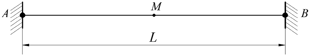
One-dimensional fixed-beam model.
Material properties of fixed-beam model.

Model loading
For the one-dimensional fixed-beam model, different points were selected at which a concentrated load was applied to produce plastic deformation. As can be observed in Figure 1, the principle of symmetry means that points on only one side of the midpoint of the beam

State of a one-dimensional fixed beam before deformation.

State of one-dimensional fixed beam after deformation due to load
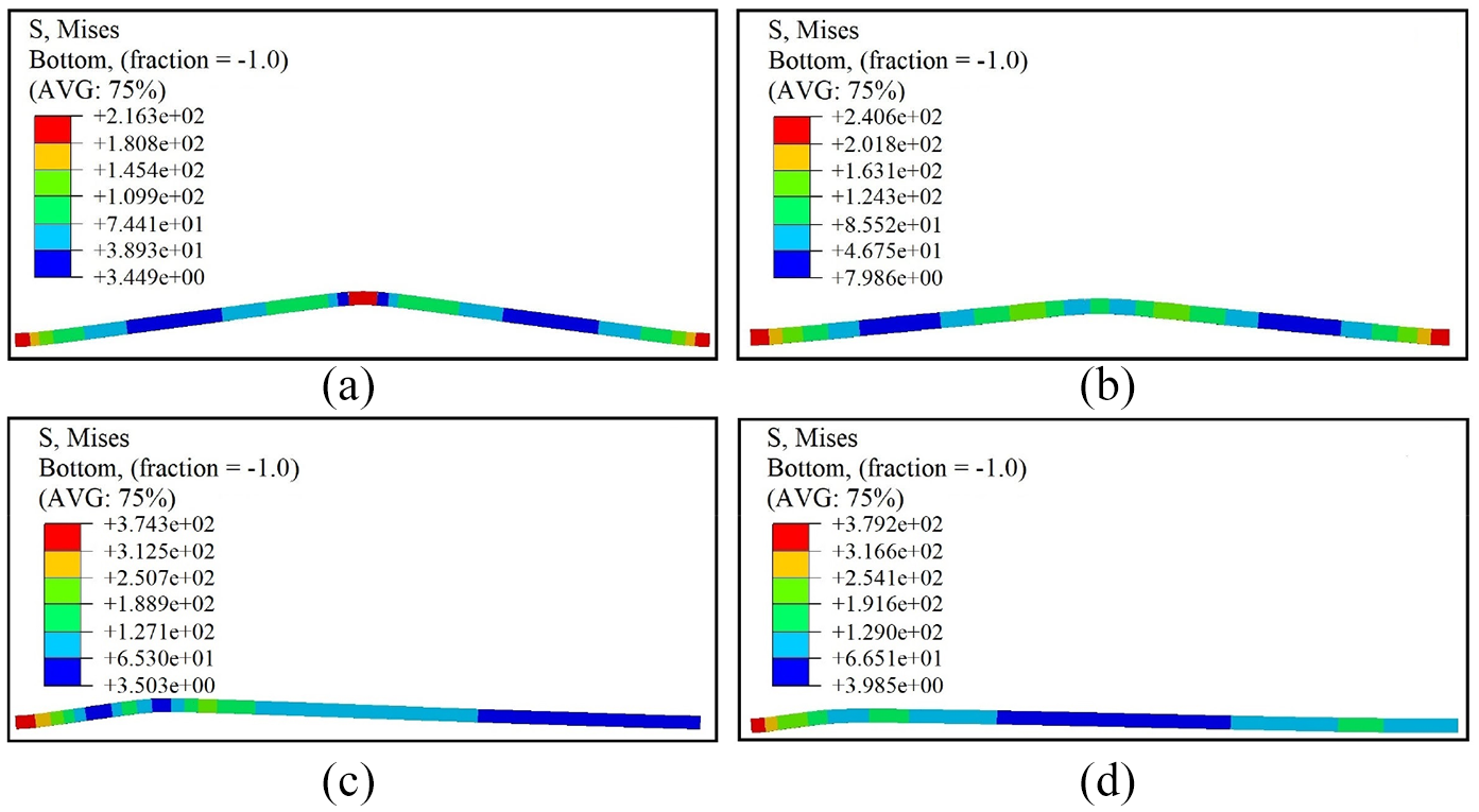
Example deflection diagrams of finite-element analysis models. (a) The first example of model analysis. (b) The second example of model analysis. (c) The third model analysis example. (d) The fourth model analysis example.
A total of 50 points were equally spaced along the

Amplitude of concentrated load application over time.
Function fitting of fixed-beam deformation curves
A polynomial is a simple continuous function that fits curves quite well as its geometric characteristics are smooth. Accordingly, in this study, we chose to use a polynomial to fit the one-dimensional fixed-beam deformation curve. The polynomial expression for the fitted curve is as follows:

where
Commonly used indicators to evaluate the fit of a function to a curve include:
(1) Root mean squared error (RMSE): This statistical parameter is the standard deviation of the regression system. 41 The closer the RMSE is to zero, the more accurate the data is fitted. The RMSE is calculated by:

where
The RMSE method based on the error between the predicted and original values. The indicators that represent the quality of fit of the curves can also be evaluated in such a way that all errors are relative to the average of the original data as follows:
(2) R-squared (R2): This statistical parameter is defined as the ratio between the sum of the squares of the regression (RSS) and total sum of squares (TSS)42,43 as follows:

where


and
The R2 value represents the overall quality of fit of the data. It can be observed in equations (3)–(5) that R2 has a normal value range of [0,1], in which a value closer to one represents a stronger ability of the equation to reflect the value of
This model is also good for data fitting. Generally, the requirement for good correlation is that R2 is greater than 0.9. In order to generate a polynomial fitting function that can not only fit the deformation curve well, but also ensure that the calculation is not too complicated, a suitable highest power n must be identified. In this study, all the models used to fit the data were developed to provide R2 values greater than 0.995. When all model fittings satisfied this requirement, the minimum value of n was eight. Therefore, this study selected an eighth-power polynomial function to fit the deformation curves. Four examples of the resulting polynomial fitted curves compared to the data are shown in Figure 6.
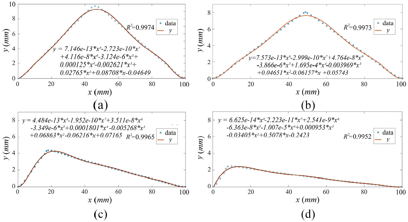
Eighth-power polynomial function fitting examples. (a) The first example of function fitting. (b) The second example of function fitting. (c) The third function fitting example. (d) The fourth example of function fitting.
To evaluate the fitted curves according common indicators RMSE and R2 above, 40 samples were randomly selected, and the RMSE and R2 values were calculated. The results, shown in Figure 7, indicate an average RMSE value of 0.11149 and average R2 value of 0.9968. Therefore, the use of the polynomial function satisfies the accuracy requirements, and the polynomial expression of the fitted curve can be defined as:


Fitting function evaluation results.
Prediction algorithm design, implementation, and verification
In this study, an algorithm flow for predicting the load magnitude and location resulting in a given plastic deformation of a one-dimensional fixed beam was designed as shown in Figure 8. Of these samples, 400 were randomly selected as training samples, and 40 of the remaining 76 cases were randomly selected as testing samples for the neural network.

Flow chart of the prediction algorithm for the large deformation of a fixed beam.
Neural network design
An artificial neural network (ANN) is a computational network with a structure that simulates biological neurons to learn the relationship between input data and output data, and is a very effective tool for predicting output data when a large set of training data are given. A typical ANN consists of types of three layers: the input layer, hidden layers, and output layer. The input layer receives external data, the hidden layers provide a complex network structure to simulate the nonlinear relationship between the input data and output data, and the output layer generates the output data. 45 A BP-ANN is a multilayer feedforward network trained by error back propagation, and is frequently used to address complex nonlinear relationships between multiple variables.46–48 Its basic principle is the gradient descent method, which uses gradient search technology to minimize the target error of the actual output value of the network against the expected output value.
In this study, the relationship between the magnitude and position of the applied load and the coefficient of the polynomial function of the curve was determined using the BP-ANN. Because the model object is a one-dimensional beam element, there is one load magnitude parameter
Training sample neural network
An initial neural network was trained using the 400 models generated and selected as detailed in Section 2.2. At this time, there were two input nodes (

Training sample neural network.
The training steps for the initial neural network were as follows:
Develop input: Collect 400 training samples to construct the relationship model between the load magnitude and location as the input layer and the polynomial coefficients as the output layer.
Construct the BP-ANN and set network parameters: Set the number of neural network layers to four: one input layer, two hidden layers, and one output layer. The input layer of the neural network consists of two nodes: the load magnitude parameter and the load location parameter. The output layer consists of the polynomial function coefficients, making nine nodes. The number of hidden layer nodes is set to 20.
Set training parameters and train the network: Set the training accuracy requirement to
Run the BP-ANN and evaluate the data processing accuracy of the established initial neural network model.
The training results are shown in Figure 10, in which it can be observed that after 16 epochs, the relative standard deviation of the training set is 0.99769 and the training accuracy reaches

Training results of the iteration calculation of the initial neural network.
As the above results demonstrate, the initial neural network training indicated a good fitting effect. Sample expansion was then performed based on Latin hypercube Sampling (LHS) to increase the number of samples input into the neural network from 400 to 2000. 49 Then, the data from the initial neural network was used to evaluate and capture the relationships within the expanded data set as detailed in Section 4.3.
Neural network for load magnitude and location prediction
A neural network for load magnitude and location prediction was trained using the 2000 samples. To then predict the load magnitude and location resulting in the observed plastic deformation of a one-dimensional fixed beam, the input layer of the neural network contained nine nodes (

Neural network for predicting load magnitude (
The training and validation steps of the predictive neural network were as follows:
Develop input: Obtain 2000 training samples by expanding the initial 400 samples based on LHS in order to construct a more accurate relationship model between the polynomial coefficients of the input layer and load magnitude and location of the output layer.
Construct the BP-ANN and set network parameters: The number of neural network layers was set to four: one input layer, two hidden layers, and one output layer. The input layer consists of the nine polynomial function coefficients as nodes. The output layer consists of two nodes, the load magnitude parameter and load location parameter. Again, there are 20 nodes in each of the two hidden layers.
Set training parameters and train the network: Set the maximum number of training steps to
Run the BP-ANN and evaluate the established predictive neural network model based on the expanded sample set.
The results are shown in Figure 12, in which it can be seen that after 93 epochs, the relative standard deviation of the training set is 0.99761 and the training accuracy is 0.0014527, indicating that the predictive neural network is well-fit to the results. The prediction and verification of the stress point of the fixed beam under large deformation can accordingly be carried out with confidence.
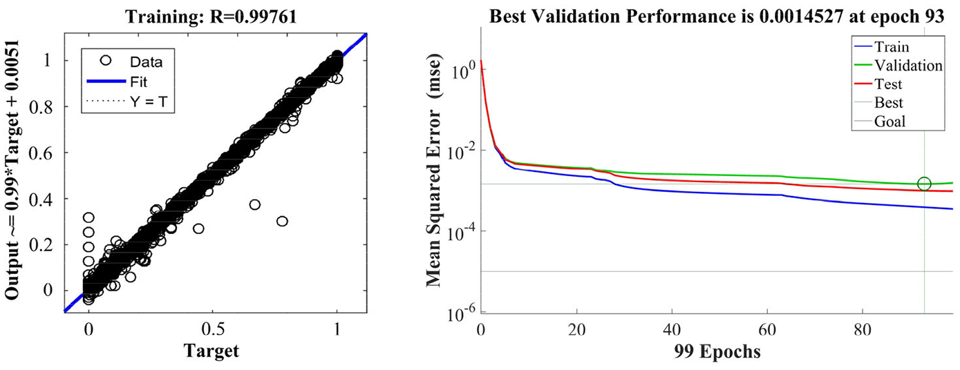
Prediction results of the iterative calculation of the neural network.
In this study, 40 sets not used in the training sets to evaluate the predictions of the trained neural network. The load magnitude and location relative errors

Comparison of the algorithm-predicted and finite-element determined actual load magnitudes and locations for the plastic deformation of a one-dimensional fixed beam.
To more closely analyze the prediction results in Figure 13, the relative and average errors of the predicted load magnitude and location were calculated by, respectively:


where
The errors calculated by equations (8) and (9) are shown in Figure 14. The maximum relative and average error of the predicted load location is
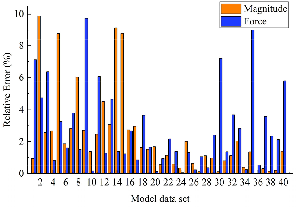
Relative errors of predicted load magnitude and location.
Conclusions
This study addresses the difficulty of determining the location and magnitude of a load on a fixed beam necessary to cause plastic deformation. A load magnitude and location BP-ANN prediction algorithm based on the series of finite element models of highly deformed one-dimensional fixed beams was accordingly constructed based on the principles of reverse engineering. The BP-ANN was initially trained using a set of 400 applied load magnitudes and locations to capture their relationships to their associated deformations as described by the coefficients of a polynomial fitting curve function. The training sample set was then expanded to 2000 items based on LHS to train the BP-ANN to predict load magnitude and location based on these coefficients. The accuracy of the load magnitudes and locations predicted by the proposed algorithm was then confirmed by comparison to the results from the finite element models. The results of this study can be summarized as follows:
Based on the analysis of the plastic deformations of a one-dimensional fixed-beam finite element model, a polynomial function fitting expression was derived to describe deformation geometry. This provided a quantitative description of plastic deformation that could be used as input to the BP-ANN.
Using the principle of reverse engineering, a BP-ANN was forward trained on a set of finite element modeling data samples to predict the polynomial coefficients describing deformation based on load magnitude and location. Then, more loads and positions are extracted as the input of the forward BP-ANN based on the LHS, the data set of the reverse training sample is expanded, and the reverse training is performed. This approach effectively addresses the problem of insufficient neural network samples under normal circumstances.
To predict the load magnitude and location required to produce plastic deformation in a one-dimensional fixed beam, an algorithm flow with high reliability was proposed. The load magnitudes and locations predicted by the algorithm and provided by the finite element analyses were compared, confirming the accuracy of the algorithm. The prediction algorithm proposed in this study thus provides a promising new approach for determining the load magnitude and location required to produce plastic deformation in a rigid body.
For further studies, we will develop models using different beam supports and large beam cross-sectional areas, and extend the model to 2D and 3D scenarios for research. The method proposed in this paper is used to analyze the cause of plastic deformation of the beam and determine the initial collision conditions. In engineering practice, the permanent plastic deformation of the general beam is known, but the load is unknown. According to actual data, the method can be used to obtain the precise size and position of the collision load, which has important practical significance. For example, the deformation of the longitudinal beam in the car, the accurate collision load and position, can help the traffic police determine the responsibility for the accident. The deformation of the beams of the bridge and the accurate collision load and location can help designers and construction personnel repair the bridge. The deformation conditions in the rail beam of the gantry crane and the wing spar of the aircraft can obtain accurate collision load and position, which can help designers improve the level of product design.
Footnotes
Declaration of conflicting interests
The author(s) declared no potential conflicts of interest with respect to the research, authorship, and/or publication of this article.
Funding
The author(s) disclosed receipt of the following financial support for the research, authorship, and/or publication of this article: Authors gratefully appreciate the support of Xi’an key laboratory of modern intelligent textile equipment (2019220614SYS021CG043), Natural Science Foundation of Shaanxi Province (2019JM-377), Postgraduate Tutor guidance ability improvement plan at Northwestern Polytechnical University (2019), China National Textile and Apparel Council (2019061) and Science & Technology Research Program in Xi’an City (2020KJRC0017).