Sage Journals: Discover world-class research

Abstract

Due to imperfect design norms and guidelines for China’s truck escape ramp, previous studies have not been able to reflect the effect of wheel subsidence process on the deceleration of runaway vehicles. A discrete element method was used to establish an aggregate discrete element and a wheel discrete element. The three-dimensional discrete element model for an aggregate-wheel combination was established based on a particle flow code in three dimensions on a software platform using the “FISH” language. The microscopic parameters of the aggregate discrete element particles and wheel discrete element particles were calibrated using a simulated static triaxial compression test and real vehicle test data, respectively. Four sets of numerical simulation tests were designed for analyzing the influence of the aggregate diameter, grade of the arrester bed, truckload, and entry speed on the wheel subsidence depth and stopping distance of runaway vehicles. The results indicate that the smaller the aggregate diameter and entry speed and the greater the truckload and grade of the arrester bed, the more easily the wheel falls into the gravel aggregate, the better the deceleration effect, and the smaller the stopping distance. As the wheel subsidence depth increases, the speed at the unit stopping distance decreases more quickly. The maximum subsidence depth mainly depends on the truckload. The research results can provide a theoretical basis for the design of the arrester bed length and the thickness of the aggregate pavement in a truck escape ramp.

Keywords

Truck escape ramp highway safety discrete element method numerical simulation

Graphical abstract

Introduction

A truck escape ramp enables trucks with brake failures to be separated from a main lane in a continuous long downhill section, allowing them to safely stop to ensure the safety of the driver’s life.^1,2 The most fundamental cause of an accident for a runaway vehicle on a truck escape ramp is that the arrester bed length setting and aggregate paving are unreasonable.^3,4 Therefore, accurately estimating the stopping distance of a runaway vehicle on an arrester bed and the wheel subsidence depth are the keys to rationally designing a truck escape ramp.

Currently, there are some methods for designing an arrester bed length: real vehicle tests, engineering experience methods, and numerical simulations. After the world’s first truck escape ramp was built in California in 1956, the United States used a large number of real vehicle tests to guide the construction of ramps.^5–7 However, this approach is unrealistic, as its engineering cost is too high. The most commonly used engineering experience method is the empirical formula for the length of an arrester bed of a truck escape ramp recommended by the Federal Highway Administration, but the results in the estimated length of the arrester bed being too small, which is unsafe for engineering applications.⁸ Al-Qadi and Rivera-Ortiz^9,10 used a triaxial test to calibrate the parameters of an arrester bed aggregate and discussed the influence of the aggregate characteristics on the stopping distance. On this basis, a semi-empirical model of a runaway vehicle running on an arrester bed was established. With the rapid development of computer science, domestic scholars have tried to estimate the length of an arrester bed using a discrete element method and have achieved some results. Zhang et al.¹¹ established a two-dimensional discrete element model for an aggregate-wheel to determine a design method for arrester bed length. Chen¹² and Qin et al.^13,14 used a two-dimensional particle flow code (PFC^2D) and TruckSim to jointly establish an aggregate-wheel two-dimensional discrete element model and to analyze the effects of aggregate type, aggregate diameter, arrester bed grade, and entry velocity on the stopping distance. Liu et al.¹⁵ established a two-dimensional aggregate-wheel discrete element model based on the discrete element method to study the thickness, length, and particle material selection of an arrester bed aggregate, and to provide corresponding recommended values.

Presently, the problem of the thickness of aggregate paving mainly refers to related foreign literature and recommended values from real vehicle tests. The Design specification for highway alignment¹⁶ indicates that the aggregate thickness at the entrance of a truck escape ramp should be 0.075 m, the maximum thickness should not be less than 1 m, and the thickness of the paving should be gradual (in the range of 30 m–60 m) along the length of the arrester bed. Hu¹⁷ gave suggestions for the thickness of aggregates through a real vehicle test method. At present, however, there are relatively few studies on the subsidence depth of the wheel in the aggregate that use numerical simulations to guide the aggregate paving of the arrester bed.

In summary, the introduction of the discrete element method for studying the deceleration of a runaway vehicle on a truck escape ramp arrester bed has proven to be feasible. However, owing to the limitations of the two-dimensional discrete element model, only the three-dimensional discrete element model can be used to study the wheel subsidence depth. To this end, a segmentation modeling method is used in a particle flow code in 3 dimensions (PFC^3D) to establish an aggregate-wheel three-dimensional discrete element model. The deceleration process of a runaway vehicle on a truck escape ramp arrester bed is numerically simulated. The resulting stopping distance and wheel subsidence depth are used to guide the design of the truck escape ramp.

Methodology

The discrete element method is a non-continuous numerical simulation method proposed by American scholar Cundall P.A. in 1971 and is based on the principle of molecular dynamics. This method mainly analyzes complex problems such as macroscopic damage and deformations of non-continuous bodies from a microscopic point of view;^18,19 thus, it can be applied to the numerical simulation of aggregate particles (non-continuous bodies) of an arrester bed. PFC^3D is a commercial software developed by the American company “ITASCA.” It uses the discrete element method and spherical discrete element particles and is widely used in civil engineering and material engineering.^20,21

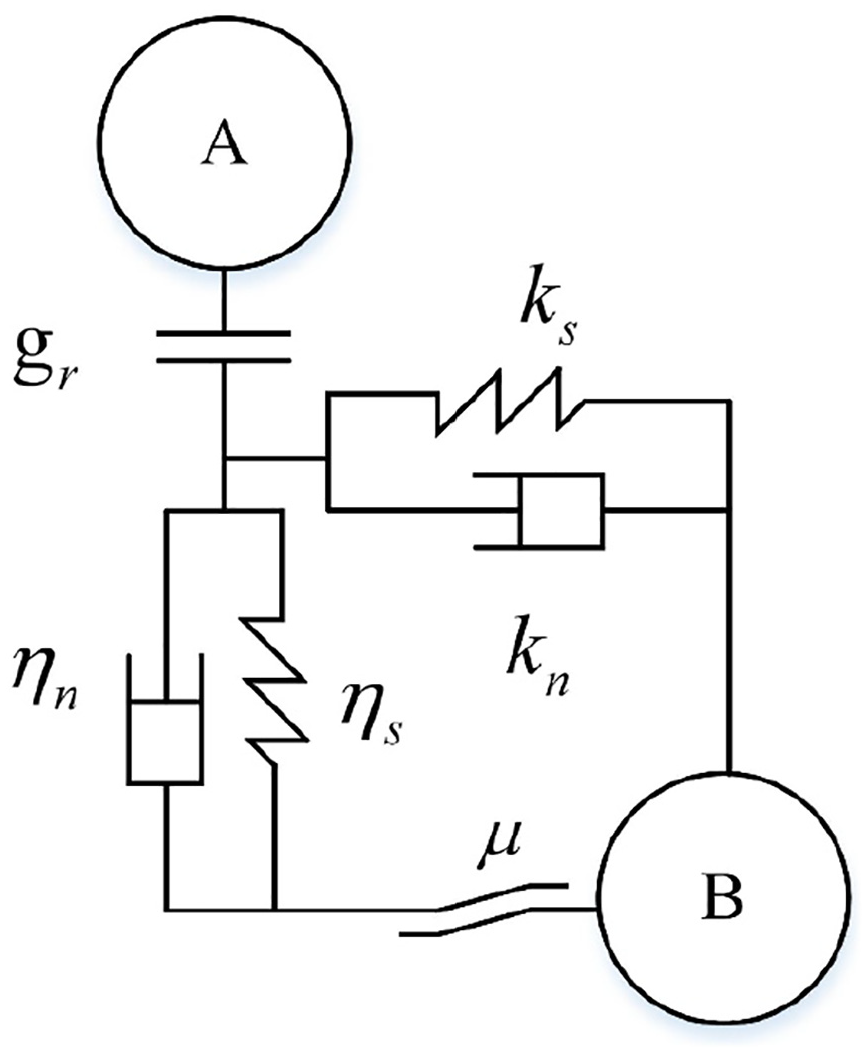
The PFC^3D assumes that the aggregate discrete element particles are rigid spheres, and that the contacts are soft contacts. It allows for a small amount of overlap, that is, the amount of overlap is small relative to the sizes of the particles themselves. PFC^3D provides a variety of contact models, such as a linear model, bonded model, and flat joint model. It is assumed that the aggregate is well-maintained on the arrester bed of the truck escape ramp, and there is no case of aggregate hardening caused by long-time use or bad weather, such as rain or snow, and so on. Therefore, the linear contact model can be adopted for simulating the mutual contact between aggregate particles in the simulation. The contact model is shown in Figure 1.

Figure 1.

Schematic diagram of linear contact model.

In Figure 1, g_r is the contact judgment parameter, and the contact model will only work when the distance between particles is less than g_r. The normal force between particles is as follows

F_{n} = \frac{k_{n, A} k_{n, B}}{k_{n, A} + k_{n, B}} x_{n} + η_{n} {\overset{\cdot}{x}}_{n}

(1)

Here, k_n,A and k_n,B are the normal stiffnesses of particles A and B, respectively; η_n is the normal damping between the particles; and x_n is the normal relative displacement between the particles.

The tangential force between particles is as follows

F_{s} = {\begin{matrix} \frac{k_{s, A} k_{s, B}}{k_{s, A} + k_{s, B}} x_{s} + η_{s} {\overset{\cdot}{x}}_{s} | F_{s} | < μ | F_{n} | \\ sign (x_{s}) . μ | F_{n} | | F_{s} | \geq μ | F_{n} | \end{matrix}

(2)

In the above, k_s,A and k_s,B are the tangential stiffnesses of particles A and B, respectively; η_s is the tangential damping between particles; x_s is the tangential relative displacement between particles; and μ is the interparticle friction coefficient. When |F_s| < μ|F_n|, the tangential force between particles is determined by the stiffness and damping; when |F_s| ≥μ|F_n|, the tangential force between particles is determined by the friction coefficient.

Considering the integrity and continuity of the wheel discrete element, the traditional contact mechanics model needs to be modified. In particular, the particles have no relative angular velocity,²² and the interparticle constitutive relationship is shown in Figure 2.

Figure 2.

Constitutive relationship between wheel model particles.

In PFC^3D, the coordinates of each particle are updated at every other time step Δt, and the velocities and accelerations of the particles are considered constant within the time step Δt. The law of particle motion follows Newton’s second law and the force-displacement law. Taking the time step Δt as the period, an explicit time center difference method cyclic calculation can solve for the motion process of the aggregate discrete element particles.

Considering the integrity of the wheel discrete element model, there are some restrictions on the range of motion for the discrete element particles. Put another way, a critical distance is required between the particles to maintain a relatively balanced position. The centroid distance between the particles is l₀. When the distance between the particles is l < l₀, a repulsive force is generated between the particles; when the distance between the particles is l > l₀, suction is generated between the particles. This assumption is made to ensure the integrity of the wheel discrete element model. A schematic motion diagram of the wheel discrete element particles is shown in Figure 3.

Figure 3.

Motion schematic diagram of wheel model particles.

Aggregate-wheel three-dimensional discrete element model

Principle of deceleration of runaway vehicles

According to a force analysis of a runaway vehicle on an arrester bed, kinetic energy can be consumed in the following ways: kinetic energy conversions between the wheel and the aggregate particles, compaction resistance, bulldozing resistance, side-shearing resistance, grade resistance, air resistance, and rolling resistance.⁹ When the wheel rolls, there will be rolling resistance and air resistance. The truck escape ramp has a certain grade; hence, the component of the wheel gravity along the grade of the arrester bed is the grade resistance. Considering the amount of wheel sinking Z, the bottom of the wheel will compact the loose aggregate to produce compaction resistance. Part of the loose aggregate accumulated in front of the wheel movement will cause the wheel’s speed to consume the wheel’s kinetic energy, and some will be pushed aside by the wheel; hence, the wheel will be subjected to bulldozing resistance. When the wheel pushes loose aggregates, it must overcome the side-shearing resistance of the aggregate to do work, further consuming kinetic energy. The principle of deceleration is shown in Figure 4.

Figure 4.

Diagram of deceleration principle.

Steps of modeling

Steps for establishing the wheel discrete elements

The wheel discrete element modeling is carried out with the 1100R20 radial truck wheel considered as the research object, and the wheel model is designed a particle cluster model based on the discrete element method to simulate the contact between the radial wheel and the aggregate. Many spherical particles of a certain particle size are superimposed into a particle cluster of a wheel model. The position of each spherical particle is calculated using MATLAB software according to the relevant formulas. The particle cluster model discretizes the contact portion between the wheel and the arrester bed aggregate and discretizes the contact force distribution between the tire particles and the aggregate particles, thereby making the contact force distribution more uniform. The steps to build the wheel model are as follows.

The parameters of the wheel discrete element are as follows: the radius is 0.55 m, the width is 0.3 m, the moment of inertia is 23.6 kg.m², the load index is 140/137, the speed symbol is K, the wheel pressure is 900 kPa, and the center coordinate of the model is taken as (0,0,0).

Many spherical particles, each with a radius of 0.05 m, are superimposed into a particle cluster of the wheel discrete elements. The position of each spherical particle in the first layer of the particle cluster can be calculated using equations (3)–(5)²³

x_{n} = (R - r) \cos θ, R_{min} \leq r \leq R_{max}

(3)

z_{n} = (R - r) \sin θ, R_{min} \leq r \leq R_{max}

(4)

R = R_{min} + 0.05 n, n = 0, 1, 2, 3, 4, 5

(5)

In the above, x_n and z_n are the coordinates of the particles in the nth layer in the xoz plane of the wheel. R is the outer edge radius of the current particle cluster, R_max is the distance from the center of the outermost circle of the particle cluster to the center of the model (here, R_max = 0.5 m), R_min is the distance from the center of the innermost particle of the particle cluster to the center of the model (here, R_min = 0.3 m), and θ is the center angle of the particle. The difference between the central angles of adjacent particles is set as π/45.

Using a loop statement, step (2) is repeated to generate six layers of particles in the xoz plane. Then, five layers of particles were generated in the Y-axis direction, by using FISH language programming in PFC^3D. The center distance between each adjacent particle layer is 0.05 m. The overlap of wheel particles is shown in Figure 5, and the wheel discrete element model is shown in Figure 6.

The particle cluster density, shear stiffness, normal stiffness, and friction coefficient are determined.

Figure 5.

Overlap of wheel particles: (a) two-dimensional diagram; (b) three-dimensional diagram.

Figure 6.

Schematic diagram of wheel element model.

Steps for establishing the aggregate discrete elements

When using the PFC^3D for simulation, the maximum number of particles recommended by ITASCA is 1 million. If a full-size arrester bed model is built, the number of particles produced will far exceed that number. To improve the calculation speed, the aggregate discrete element adopts segmentation modeling. That is, a piece of the aggregate discrete element in the PFC^3D is randomly generated using the programming language. A loop statement is used to automatically generate a next piece of the same size for the aggregate discrete element when the wheel discrete element runs halfway through a certain segment of the aggregate element, and to delete the previous piece, until the simulation motion stops. A schematic diagram of the simulation process is shown in Figure 7.

Figure 7.

Simulation motion process.

The aggregate used in this study is river pea gravel, and assumes that the aggregate discrete element particles are rigid spheres. The steps of establishing the aggregate discrete element are as follows.

Generating walls. Five walls are generated: front, back, left, right, and bottom. The dimensions of each wall are 2000 × 1200 × 600 mm. Then, the five walls are given a normal stiffness, shear stiffness, and friction coefficient.

Recording wall information. The vertex positions, size, shear stiffnesses, normal stiffnesses, and friction coefficients of the five walls are recorded.

Generating balanced aggregate. An aggregate with an average diameter of 20 mm is randomly generated for the established wall. The gravitational acceleration in the z direction is set to g_z = −9.81 m/s², and the gravitational accelerations in the x and y directions are both 0. When the ratio of the average sum of the contact force and the volume force of all the particles to the sum of the contact force and the volume force applied to the particles is less than 0.01%, the aggregate is considered to have reached equilibrium.

Recording particle information. The density, radius, position, normal stiffness, shear stiffness, and friction coefficient of each particle in the aggregate are recorded.

Generating and deleting the aggregate cyclically. When the wheel is running forward, the running distance of the wheel is determined. When the distance reaches (2n+ 1, n = 1, 2, 3…), the data obtained in step (2) and step (4) are used to quickly generate the next section of the aggregate and the wall. The newly generated walls and particles move in the x and z directions, but the relative positional relationships between the particles themselves and the particles and the walls remained unchanged; thus, the newly generated aggregate is in equilibrium. When the running distance of the wheel discrete element reaches 4 m or more, after the next pieces of aggregate and walls are generated, the aggregated particles and wall that have been passed through are simultaneously deleted. During the simulation, the length of the arrest bed is kept at 4 m until the wheel stops moving.

Simulation model

After the wheel discrete element and the aggregate discrete element are, respectively, established in the above two sections, the aggregate-wheel three-dimensional discrete element model can be established, as shown in Figure 8.

Figure 8.

Model of three-dimensional discrete element.

Model calibration

The calibration of the 3D discrete element model is divided into two stages. The first stage uses a simulated static triaxial compression experiment to calibrate the micro-parameters of the aggregate discrete element particles. The second stage uses real vehicle test data to calibrate the micro-parameters of the wheel discrete element. The real triaxial compression test data and real vehicle test data used in the calibration process are derived from the test data of Al-Qadi and Rivera-Ortiz.^9,10

Calibration of micro-parameters of the aggregate discrete element particles

The microscopic parameters of the aggregate discrete element particles include the particle density, shear stiffness, normal stiffness, and friction coefficient. To calibrate the microscopic parameters of the particles, a virtual triaxial compression model was generated at the same size as the laboratory triaxial compression test, as shown in Figure 9. Three sets of numerical simulation triaxial compression tests were conducted in the PFC^3D software. The test conditions were as follows: (a) the relative densities for the three sets of tests were 13%, 45%, and 80%, respectively; and (b) the confining pressures were 69, 137, and 206 kPa, respectively. In the simulation of triaxial compression, the upper and lower walls compressed the test piece at a certain speed, and the cylindrical wall continuously maintained a certain lateral confining pressure via the servo principle. The triaxial compression test was carried out under the different relative densities and different confining pressures mentioned above. After adjusting the micro-parameters of the particles several times, the peak stress and peak strain of the simulated gravel and real gravel were as close as possible, and the triaxial compression was completed. The results of the triaxial compression test are shown in Table 1. The calibration results for the micro-parameters of the aggregate discrete element particles are shown in Table 2.

Figure 9.

Simulation triaxial compression model.

Table 1.

Triaxial compression test results.

Relative densities (%)	Confining pressures (kPa)	Peak stress (kPa)		Peak strain		Volumetric strain
		Real data	Simulation data	Real data	Simulation data	Real data	Simulation data
13	69	294	271	0.044	0.039	−0.00225	−0.0068
	137	480	481	0.055	0.040	−0.00290	−0.013
	206	571.1	720	0.063	0.053	−0.00860	−0.0094
45	69	324	280	0.039	0.036	+0.00105	−0.0031
	137	659	608	0.055	0.039	+0.00130	−0.0090
	206	701	800	0.058	0.049	+0.00190	−0.011
80	69	367	348	0.033	0.035	+0.00615	0.00128
	137	772	686	0.041	0.037	+0.00650	−0.0029
	206	986	1011	0.053	0.046	+0.02170	−0.016

Table 2.

Micro-parameters of aggregate discrete element particles.

Average diameter (mm)	Density(kg/m³)	Normal stiffness(N/m)	Shear stiffness(N/m)	Frictioncoefficient
20	2500	2.0e6	2.5e6	0.75

It can be seen from Table 1 that the three-dimensional simulation triaxial compression calibration results are basically consistent with the real triaxial compression experimental data. Moreover, the micro-parameters of the aggregate discrete element particles meet the simulation requirements.

Calibration of microscopic parameters of the wheel discrete element particles

According to the dynamic equation of the linear contact model, the microscopic parameters of the wheel discrete element particles mainly include the normal stiffness, tangential stiffness, and friction coefficient. The real vehicle test conducted by Al-Qadi was conducted under the condition that the arrester bed grade was 0, and at a certain truckload and entry speed. By using the calibrated aggregate discrete element particles to simulate the wheel discrete element particles, the micro-parameters of the wheel discrete element particles were adjusted according to the stopping distance, average acceleration, maximum sinking, and average sinking of the real vehicle test; hence, each indicator was close to the real vehicle data. The results are shown in Figure 10.

Figure 10.

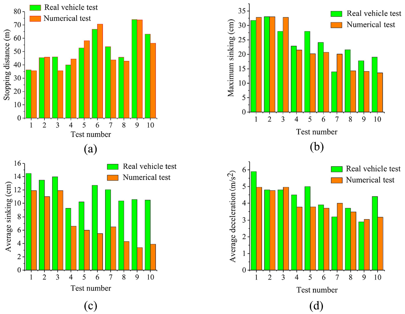
Real vehicle test and numerical simulation: (a) stopping distance; (b) maximum sinking; (c) average sinking; (d) average deceleration.

The correlation coefficient (ρ_r) between the four above indicators and the corresponding real vehicle data are shown in Table 3. Among the four indicators, the correlation coefficients between the stopping distance, maximum sinking, and average deceleration and the corresponding real vehicle data are all greater than 0.8, that is, highly correlated. The correlation coefficient between the simulated average sinking and the actual vehicle data is 0.69, that is, moderately correlated. The main reason is that in the real vehicle test, each rut is run over by two or more wheels; thus, the average rut depth measured after the end of the test is much larger than that for a numerical simulation test of a single wheel.

Table 3.

Correlation coefficient between simulated data and real vehicle data.

	Stopping distance	Maximum sinking	Average deceleration	Average sinking
ρ_r	0.91	0.81	0.85	0.69

The relative error of the data of Figure 10 is compared with the relative error of the corresponding data of the two-dimensional discrete element model established in Zhang et al.¹¹ The results are shown in Table 4.

Table 4.

Comparison of relative errors between 2D model and 3D model.

Indicators	3D model	2D model	Comparison of results
Stopping distance	0.0887	0.0895	−0.0008
Average deceleration	0.1296	0.2098	−0.0802
Maximum sinking	0.1741	0.6514	−0.4773
Average sinking	0.4132	0.5972	−0.184

It can be seen from Table 4 that in terms of stopping distance, the simulation results of the two-dimensional and three-dimensional discrete element models are not very different, and that both can achieve good results. However, in terms of average deceleration, maximum sinking, and average sinking, the three-dimensional discrete element model is superior to the two-dimensional model. The three-dimensional discrete element model can represent the subsidence deformation of the wheel, whereas the two-dimensional model cannot. For the force deceleration process of a runaway vehicle on the arrester bed of a truck escape ramp, the wheel subsidence deformation will affect the stopping distance; thus, the three-dimensional discrete element model can estimate the stopping distance more accurately than the two-dimensional model.

Figure 11 shows the change process of the wheel subsidence depth in test No. 1.

Figure 11.

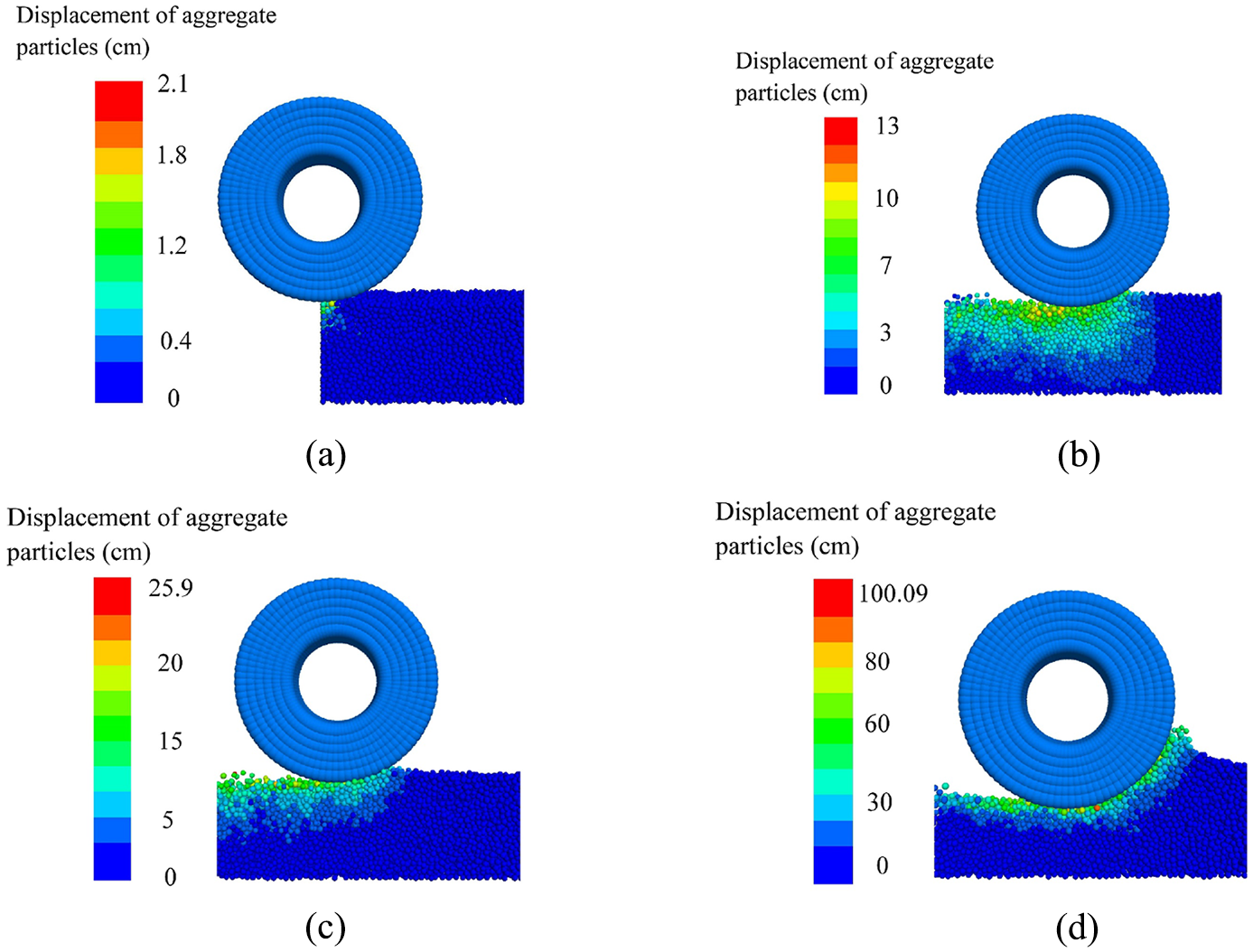
The change process of wheel subsidence depth in test No. 1: (a) driving distance is 0 m; (b) driving distance is 2.5 m; (c) driving distance is 20 m; (d) driving distance is 35.6 m.

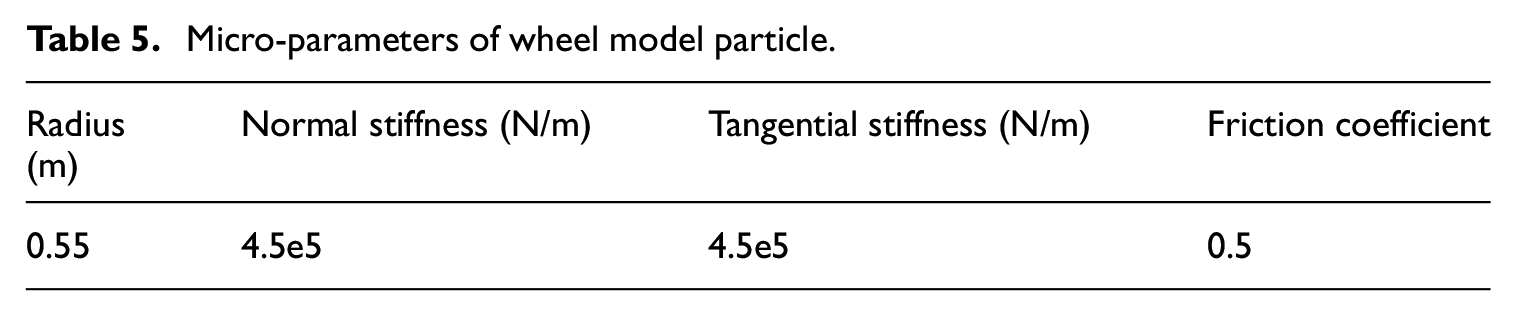
From the above simulation analysis, it can be observed that the microscopic parameters of the wheel discrete element particles can provide numerical simulation results closer to the real vehicle full-scale test data to better realize the numerical simulation of the deceleration process of a runaway vehicle on the arrester bed of a truck escape ramp. The calibrated aggregate-wheel three-dimensional model can be used in the next step of numerical simulation. The micro-parameter calibration results for the wheel discrete element particles are shown in Table 5.

Table 5.

Micro-parameters of wheel model particle.

Radius(m)	Normal stiffness (N/m)	Tangential stiffness (N/m)	Friction coefficient
0.55	4.5e5	4.5e5	0.5

Numerical simulation and analysis

Numerical simulation scheme

Using the calibrated three-dimensional discrete element model, four sets of numerical simulations were conducted, to analyze the influences of the gravel diameter, truckload, entry speed, and arrester bed grade on the wheel subsidence depth and stopping distance. The design of the numerical simulation scheme is shown in Table 6. In Table 6, the gravel diameter is within the range of grade 57 (2.36–37.5 mm) recommended by the American Association of State Highway and Transportation Officials, USA.⁸ The Design specification for highway alignment¹⁶ recommends that the entry speed for the design of the length of a truck escape ramp should be 100 or 110 km/h, and the maximum grade of the arrester bed should not exceed 15%; hence, the maximum entry speed is 108 km/h (30 m/s) and the grade selection is 0%, 5%, and 10%. In this study, it is assumed that the centroid speed of the wheel is the entry speed, that the force of the total truckload on the wheel is applied to the wheel center and is constant, and that the influence of the suspension system is ignored. Accordingly, the truckload is the total truckload divided by the number of wheels. The truckload of a single wheel is, respectively, set as 2500 kg, 3750 kg (50% overload), and 5000 kg (100% overload).

Table 6.

Design of numerical simulation scheme.

Test	Grade (%)	Truckload (kg)	Entry speed (m/s)	Gravel diameter (mm)
1	5	2500	25	14–22
	5	2500	25	22–30
	5	2500	25	30–38
2	5	2500	25	30–38
	5	3750	25	30–38
	5	5000	25	30–38
3	5	2500	20	30–38
	5	2500	25	30–38
	5	2500	30	30–38
4	0	2500	25	30–38
	5	2500	25	30–38
	10	2500	25	30–38

Simulation results and analysis

The simulation results obtained from the test scheme of Table 6 are shown in Figures 12 –15.

Figure 12.

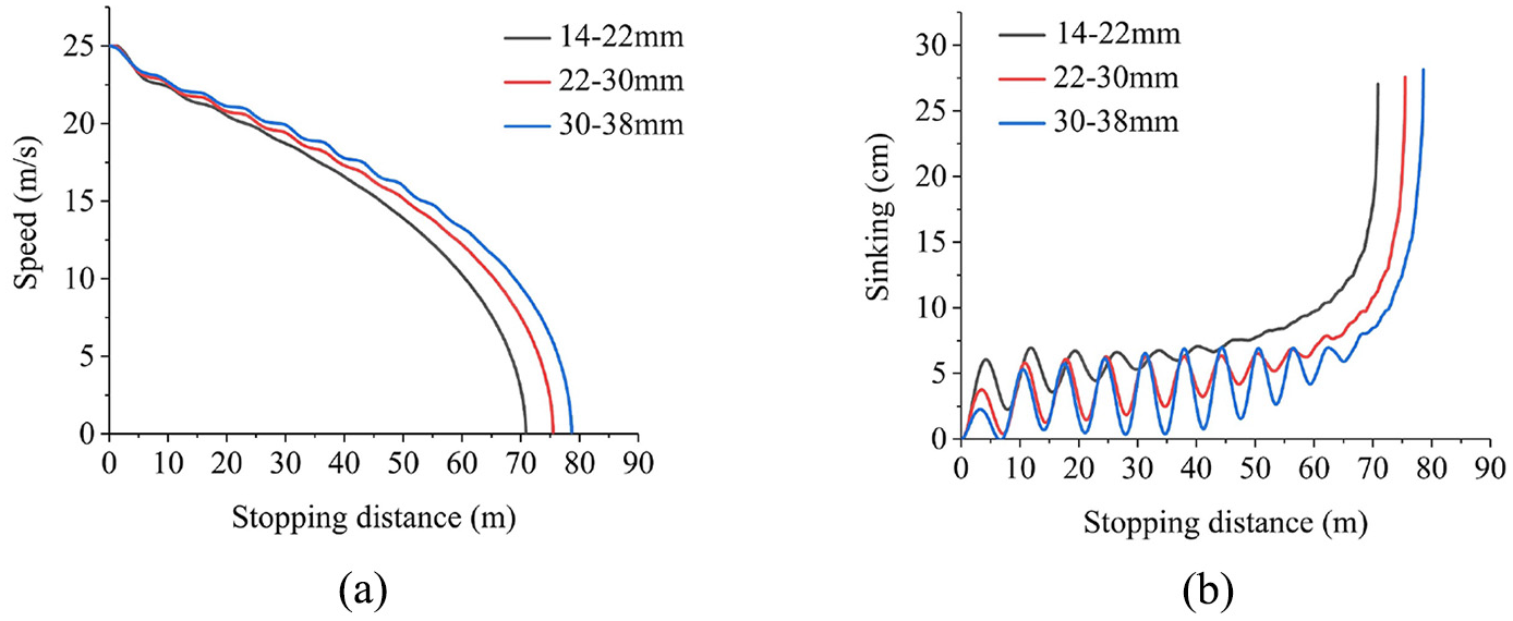
Test 1 simulation curve: (a) speed curve; (b) sinking curve.

Figure 13.

Test 2 simulation curve: (a) speed curve; (b) sinking curve.

Figure 14.

Test 3 simulation curve: (a) speed curve; (b) sinking curve.

Figure 15.

Test 4 simulation curve: (a) speed curve; (b) sinking curve.

It can be seen from Figure 12 that for a given entry speed, truckload, and grade, the smaller the gravel diameter, the smaller the stopping distance of the uncontrolled vehicle on the arrester bed. Moreover, the smaller the gravel diameter, the greater the deformation of the wheel during the deceleration and stopping, indicating that the wheel will more easily fall into the gravel aggregate. In addition, during the deceleration of the wheel, as the aggregate continues to accumulate in the front part of the wheel, the wheel subsidence deformation changes into a “wavy shape.” At the maximum value of the subsidence, the wheel speed decreases rapidly, whereas at the minimum value, the speed drops slowly. Accordingly, when the gravel diameter is small, the wheel can more easily fall into the gravel aggregate during the deceleration process. The increase in the wheel subsidence deformation causes the contact area of the wheel and the gravel particles to increase, and the resistance of the wheel increases. The kinetic energy consumption of the wheel becomes faster, and the stopping distance is reduced. However, the aggregate diameter has little influence on the maximum subsidence of the wheel. In this group of simulation tests, the maximum subsidence depth of the wheel was approximately 29 cm.

It can be seen from Figure 13 that for a given entry speed, gravel diameter, and grade, the stopping distance decreases with an increase in the truckload. In addition, the wheel sinking curve of a heavily loaded vehicle is larger than that of a vehicle with a small load. This indicates that when the vehicle enters the escape ramp under certain working conditions, the larger the load, the easier the wheel will fall into the aggregate. The contact area between the wheel and the aggregate will increase; hence, the resistance will be increased, and the stopping distance will decrease accordingly. The maximum subsidence also increases with an increase in the truckload. When the load of a single wheel is 2500 kg, the maximum subsidence depths are 30 cm, 40 cm for 3750 kg, and 50 cm for 5000 kg, respectively. This proves that the truckload has a great influence on the maximum sinking. Thus, the aggregate pavement is safe for truckloads under 20 t, according to the Design specification for highway alignment.¹⁶

It can be seen from Figure 14 that for a given gravel diameter, truckload, and grade, the stopping distance increases with an increase in the entry speed. In addition, the sinking curve for a large entry speed is smaller than that for a small entry speed, but the maximum subsidence is similar. This indicates that as the uncontrolled vehicle enters the escape ramp, the greater the entry speed of the vehicle, the greater the initial kinetic energy of the vehicle, and the greater the stopping distance required to completely consume the kinetic energy. In addition, the greater the entry speed of the vehicle, the less likely the wheel will fall into the aggregate during the deceleration process of entering the ramp. The smaller the contact area between the aggregate and the wheel, the smaller the resistance, and the larger the corresponding stopping distance. However, the maximum subsidence of the wheel is approximately 30–35 cm in this group of simulation tests; hence, the impact of the entry speed on the maximum subsidence is relatively small.

It can be seen from Figure 15 that for a given gravel diameter, truckload, and entry speed, the stopping distance decreases with an increase in the grade. The greater the grade of the arrester bed, the more evident the “wavy shape” of the wheel, and the greater the subsidence during deceleration and stopping. This indicates that the larger the grade of the arrester bed, the greater the kinetic energy consumed by gravity and hence, shorter the stopping distance. A larger wheel subsidence further increases the resistance of the arrester bed, and also reduces the stopping distance. In addition, the influence of the gradient of the arrester bed on the maximum wheel subsidence is small, that is, approximately 30–35 cm in this group of simulation tests.

Conclusion

In this study, a discrete element method is used to establish an aggregate-wheel three-dimensional discrete element model based on PFC^3D software, and the deceleration process of a runaway vehicle on the arrester bed of a truck escape ramp is numerically simulated. The variation laws of stopping distance and wheel subsidence depth are obtained, providing a theoretical basis for the design of the arrester bed length in the ramp and the aggregate paving thickness of the arrester bed. The final research results are as follows.

The calibration method is simple and feasible; it merely comprises establishing the aggregate-wheel three-dimensional discrete element model, using the simulated triaxial compression tests to calibrate the microscopic parameters of the aggregate discrete element particles, and using the actual vehicle test data to calibrate the microscopic parameters of the discrete elements of the wheel.

Based on the model after calibration, the numerical simulation is conducted by means of segmentation modeling, and the variation laws of stopping distance and wheel subsidence depth are obtained. Owing to consideration of the influence of wheel subsidence deformation, the estimation accuracy of the three-dimensional discrete element model stopping distance is higher than that of the two-dimensional model.

Based on considering the influence of the wheel subsidence process on the stopping distance, the numerical simulation results show that when the runaway vehicle enters the arrester bed of the truck escape ramp under certain working conditions, a greater wheel subsidence deformation is obtained with a smaller aggregate diameter, smaller entry speed, greater truckload, or greater arrester bed grade. This indicates that the more easily the wheel falls into the gravel aggregate, the better the deceleration effect, and the smaller the stopping distance. As the wheel subsidence deformation increases, the speed of the wheel at the unit stopping distance decreases more quickly. Among the four factors, only the truckload has a significant impact on the maximum sinking.

The three-dimensional discrete element model overcomes the limitations of the two-dimensional discrete element model and can reflect the sinking deformation of the wheel during deceleration, making the process of numerical simulation closer to reality.

Footnotes

Declaration of conflicting interests

The author(s) declared no potential conflicts of interest with respect to the research, authorship and/or publication of this article.

Funding

The author(s) disclosed receipt of the following financial support for the research, authorship, and/or publication of this article: This research article is supported by the Special Project on Innovation Driven Development in Guangxi (grant number: Guike AA18242033 and Guike AA18242033-6), Guangxi Natural Science Foundation (grant number: 2019JJA160121) and Guangxi Key Laboratory of Manufacturing System & Advanced Manufacturing Technology (grant number: 19-050-44S003), which are gratefully appreciated.

ORCID iD

Pinpin Qin

Author biographies

Pinpin Qin received the PhD degrees in traffic engineering from Southwest Jiaotong University in August 2007. She is an associate professor of mechanical engineering at Guangxi University. Her research interests include vehicle dynamics and system safety.

Fengmin Wu received the Bachelor's degree in Hubei University of Technology in July 2017. He is a master degree candidate of mechanical engineering at Guangxi University. His research interests include vehicle dynamics and system safety.

Da Wu received the Bachelor's degree in Chongqing University of Technology in July 2018. He is a master degree candidate of mechanical engineering at Guangxi University. His research interests include vehicle dynamics and system safety.

Shunfeng Zhang received the Bachelor's degree in Chongqing University of Technology in July 2019. He is a master degree candidate of mechanical engineering at Guangxi University. His research interests include vehicle dynamics and system safety.

Daming Huang received the MS degrees in repair and manufacture of agricultural machinery from Guangxi Agricultural University in July 1982. He is a professor of mechanical engineering at Guangxi University and Nanning University. His research interests include transport safety.

References

Yan

Prediction model for brake-drum temperature of large trucks on consecutive mountain downgrade routes based on energy conservation law. Math Probl Eng 2018; 2018: 4587673.

Hou

Zhong

, et al. Summary of and lessons from domestic and oversea setting of truck escape ramp. Appl Mech Mater 2014; 607: 839–846.

Capuano

Heymsfield

Alternative arresting system design for truck escape ramp. Int J Crashworthines 2018; 23(6): 618–626.

Zhang

Analysis of incidents in emergency escape ramps and legal risk aversion. In: Proceedings of the fourth international conference on transportation engineering 2013 (ICTE 2013), Chengdu, China, 19–20 October 2013, pp. 706–715. Chengdu, China: American Society for Civil Engineers.

Eck

RW.

State practice and experience in the use and location of truck escape ramp facilities. Transport Res Rec 1979; 736: 34–43.

Carrier

Pachuta

JA.

Runaway trucks in Pennsylvania. SAE Trans 1981; 90: 3924–3933.

Wambold

JC.

Field study to establish truck escape ramp design methodology. Transport Res Rec 1989; 1233: 94–103.

Federal Highway Administration (FHWA). Interim guidelines for design of emergency escape ramps: T 5040.10. Washington, DC: FHWA, 1979.

Al-Qadi

Rivera-Ortiz

LA.

Use of gravel properties to develop arrester bed stopping model. J Transp Eng 1991; 117(5): 566–584.

10.

Al-Qadi

Rivera-Ortiz

LA.

Laboratory testing of river gravel used in arrester beds. J Test Mater 1991; 19(4): 280–291.

11.

Zhang

Sun

Cheng

, et al. Determining method of length of arrested bed of truck escape ramp based on particle flow simulation. Highw Transp Technol 2011; 28(10): 118–123.

12.

Chen

Study on the influence of the arrangement of shelter lane on the dynamic characteristics of vehicle systems. Nanning, China: Guangxi University, 2017.

13.

Qin

Chen

Pei

, et al. A PFC2D model of the interactions between the tire and the aggregate filled arrester bed on escape ramp. In: Proceedings of the 2017 2nd international conference on civil engineering and materials science, Seoul, Korea, 26–28 May 2017, pp. 243–249. Seoul, Korea: ICCEMS.

14.

Qin

Chen

Guo

, et al. Analyzing the influence of aggregate properties on stopping distance on truck escape ramps. J Shanghai Jiao Tong Univ 2019; 24(2): 1–5.

15.

Liu

Wang

, et al. Determination of truck escape ramp parameters in tire-particle simulation using the discrete element method. China J Highw Transp 2019; 32(2): 165–173.

16.

CCCC First Highway Consultants Co. Ltd. Design specification for highway alignment: JTG D20-2017. Beijing, China: China Communications Press, 2017.

17.

Research on setting techniques of truck escape ramp for general national and provincial highway. Chongqing, China: Chongqing Jiao Tong University, 2017.

18.

Cundall

PA.

A computer model for simulating progressive largescale movements in blocky system. In: Muller

(ed.) Proceedings of symposium of the international society of rock mechanics, Vol. 1. Rotterdam: A.A. Balkema, 1971, pp. 8–12.

19.

Cundall

PA.

The measurement and analysis of acceleration in rock slopes. PhD Dissertation, Imperial College of Science and Technology, University of London, London, 1971.

20.

Peng

Zhu

, et al. Discrete element method simulations of load behavior with mono-sized iron ore particles in a ball mill. Adv Mech Eng 2017; 9(5): 1–10.

21.

Zeng

Song

Wang

, et al. Ballast bed resistance characteristics based on discrete-element modeling. Adv Mech Eng 2018; 10(6): 1–9.

22.

Wang

The analysis of the interaction between wheel and soft ground based on DEM. Changchun, China: Jilin University, 2012.

23.

Zhang

Modeling and simulation of the interaction between wheel and sand using discrete element method. Changsha, China: National University of Defense Technology, 2015.

Three-dimensional discrete element simulation of the runaway vehicle deceleration process on the arrester bed of truck escape ramps

Abstract

Keywords

Introduction

Methodology

Aggregate-wheel three-dimensional discrete element model

Principle of deceleration of runaway vehicles

Steps of modeling

Steps for establishing the wheel discrete elements

Steps for establishing the aggregate discrete elements

Simulation model

Model calibration

Calibration of micro-parameters of the aggregate discrete element particles

Calibration of microscopic parameters of the wheel discrete element particles

Numerical simulation and analysis

Numerical simulation scheme

Simulation results and analysis

Conclusion

Footnotes

Declaration of conflicting interests

Funding

ORCID iD

Author biographies

References