Numerical calculation for coupling vibration system by Piecewise-Laplace method

Abstract

To improve the reliability and accuracy of dynamic machine in design process, high precision and efficiency of numerical computation is essential means to identify dynamic characteristics of mechanical system. In this paper, a new computation approach is introduced to improve accuracy and efficiency of computation for coupling vibrating system. The proposed method is a combination of piecewise constant method and Laplace transformation, which is simply called as Piecewise-Laplace method. In the solving process of the proposed method, the dynamic system is first sliced by a series of continuous segments to reserve physical attribute of the original system; Laplace transformation is employed to separate coupling variables in segment system, and solutions of system in complex domain can be determined; then, considering reverse Laplace transformation and residues theorem, solution in time domain can be obtained; finally, semi-analytical solution of system is given based on continuity condition. Through comparison of numerical computation, it can be found that precision and efficiency of numerical results with the Piecewise-Laplace method is better than Runge-Kutta method within same time step. If a high-accuracy solution is required, the Piecewise-Laplace method is more suitable than Runge-Kutta method.

Introduction

Any complex vibration systems can be described with differential dynamic equations. For exploring the dynamic characteristics of the vibrating system, obtaining accurate solution of the dynamic equations is crucial in engineering design. Of course, Euler’s method, Taylor-series method and Runge-Kutta method, and so on, are relatively mature methods existed in numerical analysis for vibration systems.^1,2 We can choose these computing methods to solve the problems occurred in our practical engineering. ³ Such as Euler’s method, which is the most traditional method to solve differential equations, however, numerical accuracy should be decreased as integral curve is replaced with approximated polyline in the calculation process. To perfect numerical accuracy in computing principle, trapezoidal method employ trapezoid to match integral curve in calculation process, and so the solution precision of this method is much higher than Euler’s method, but the computational efficiency is restricted on account of its own algorithm complexity and large calculating quantity. In order to improve the computation efficiency, Carl Runge and Martin Kutta proposed Runge-Kutta method, and the theoretical basis of this method is derived from the Taylor’s expansion and slope approximation;^2–4 in the solving process, the weighted average of the slope of multiple points in an integrating interval is calculated; the accuracy of the Runge-Kutta method is depended on the number of points in the integrating interval, the more points, the more accurate the calculation, and the more time needed to be taken in calculation. Since almost all terms are linearized and discontinuous when solving equations with Runge-Kutta method, calculative deviation is inevitable, ⁴ which has attracted much more attention of numerous researchers. Shampine and Watts proposed a way of local error estimators, which seems to be of broad applicability; ⁴ according to this way, an efficient computational code (ode45) is compiled, and comparing the results of traditional Runge-Kutta to ode45, solution accuracy of Runge-Kutta is defective as the obtained results are not continuous. The inherent characteristics of the system are lost in the second step of the calculation by using the Runge-Kutta method. ⁵

Considering discontinuity and inefficiency of the Runge-Kutta method, Dai and Singh proposed piecewise constant arguments to maintain solution continuity in computation process of linear system, and better reliability and accuracy of the method was demonstrated by comparing with the traditional Runge-Kutta method; ⁶ uniting the piecewise constant arguments with Taylor expansion (P–T), solution continuity and accuracy of the nonlinear system is also ensured as the piecewise constant arguments can remain the characteristics of the system in calculation process. Therefore, the P–T method is a new approach for finding approximated solution of linear and nonlinear vibration systems. ⁷ However, the study object of the P–T method is useful for multiple degree of freedom (MDOF) system with without coupled terms, but MDOF dynamic systems are commonly coupled with multiple variables in engineering practices. ⁸ Such as vibration isolation system, Chen and Zhang explored the characteristics of vibration isolation with a nonlinear energy sink moving vertically.^9–11 Fang proposed a vibrating system coupled with inertial terms to obtain ideal dynamic characteristics, but the accuracy of displacement response of the system is decreased as the original model is excessively simplified.^12,13 For a robot system with flexible components, vibration errors can be easily occurred in traditional computation methods, and the responses of the system is mainly obtained with experimental results, which should spend high design cost owing to low accuracy of analytical solution. ¹⁴ Therefore, it is necessary to develop a high-precision algorithm to solve the problem of coupled systems.

Piecewise-Laplace principle

Piecewise constant argument

Definition 1

A function $h(x_1,x_2,\dots ,x_n)$ is said to satisfy a Lipschitz condition in the neighborhood of $(x_1^0,x_2^0,\dots ,x_n^0)$ if there exists a constant L such that ⁷

$$|h(x_1,x_2,\dots ,x_n)-h(x_1^0,x_2^0,\dots ,x_n^0)|⩽L|x_i-x_i^0|$$

(1)

For any point $h(x_1,x_2,\dots ,x_n)$ in the neighborhood of $(x_1^0,x_2^0,\dots ,x_n^0)$ , where $i=1,2,3,\dots ,n$ .

Lemma 1

If h is a continuous function and satisfies a Lipschitz condition for all variables except t in the neighborhood of $t_0,y_0,y{\prime }_0,y_0^{(n-1)}$ , then, there is a unique function $y(t)$ such that ⁷

$$y(n)=h(t,y,y\prime ,\dots ,y^{(n-1)})$$

(2)

$$y(t_0)=y_0,y\prime (t_0)=y{\prime }_0,\dots ,y^{(n-1)}(t_0)=y_0^{(n-1)}$$

(3)

Theorem 1

Suppose argument [Nt] is the integer-valued function of product of time t and parameter N, where N as a positive integer. ⁷ When N is approached to infinity, the value of the argument [Nt]/N tends to t, that is

$$\underset{N\to \infty }{lim}\frac{\left[\mathrm{Nt}\right]}{N}=t$$

(4)

Proof

For any given $\epsilon$ , there exists a $N_0$ such that $1/N_0<\epsilon$ . Since $[\mathrm{Nt}]/N-t=([\mathrm{Nt}]-\mathrm{Nt})/N$ and $-1⩽[\mathrm{Nt}]-\mathrm{Nt}⩽0$ , hence, $|[\mathrm{Nt}]/N-t|⩽1/N$ . Accordingly for any $\epsilon >0$ , take $N_0⩾1/\epsilon$ , when $N⩾N_0$ . It follows that

$$|\frac{[\mathrm{Nt}]}{N}-t|⩽\frac{1}{N}⩽\frac{1}{N_0}⩽\epsilon$$

(5)

By the arbitrariness of $\epsilon$ , a result of limiting case can be given as follows

$$\underset{N\to \infty }{lim}\frac{\left[\mathrm{Nt}\right]}{N}=t$$

(6)

Remark

Theorem 1 is extremely essential for studying the relationship between piecewise constant systems and corresponding continuous systems, and most of the later derivations in this paper will depend on them.

Theorem 2

Considering a vibrating system

$$f(x″,x\prime ,x)=g(t)$$

(7)

with initial conditions

$$x(0)=d_0,x\prime (0)=v_0$$

(8)

Then, in time interval $i/N⩽t<(i+1)/N$ , equations (7) and (8) are converted to

$$f({x″}_i,{x\prime }_i,x_i)=g\left(\frac{i}{N}\right)$$

(9)

and

$$x_i\left(\frac{i}{N}\right)=d_i,x{\prime }_i\left(\frac{i}{N}\right)=v_i$$

(10)

where i = 0, 1, 2, . . ., [Nt].

Proof

According to Definition 1 and Lemma 1, the function $f({x″}_i,x{\prime }_i,x_i)$ satisfies a Lipchitz condition for $x{\prime }_i$ and $x_i$ . Therefore, there must exist a unique solution for equation (9). In addition, because of the existence and uniqueness of the continuous differential equations, equation (10) can be derived.

Remark

Theorem 2 plays an important role in determining the local initial conditions of a piecewise constant system.

Laplace transformation and residues principle

The coupling system can be decoupled with the Laplace transformation. ¹⁵ And some significant theorems should be stressed.

Theorem 3

Supposing functions ${x″}_i(t)$ , $x{\prime }_i(t)$ and $x_i(t)$ can be rewritten as Laplace style,^16,17 that is

$$L[x_i(t)]=X_i(s)$$

(11)

$$L[{x\prime }_i(t)]=s{X}_i(s)-x_i\left(\frac{i}{N}\right)$$

(12)

$$L[{x″}_i(t)]=s^2{X}_i(s)-s{x}_i\left(\frac{i}{N}\right)-x{\prime }_i\left(\frac{i}{N}\right)$$

(13)

where ${x″}_i(t)=\frac{d^2{x}_i}{d{t}^2},x{\prime }_i(t)=\frac{d{x}_i}{\mathrm{dt}}.$

Proof

According to the definition of Laplace transformation,

$$\begin{array}{c}(1)L[x_i(t)]=\underset{i/N}{\overset{\infty }{\int }}{e}^{-\mathrm{st}}{x}_i(t)\mathrm{dt}=X_i(s)\hfill \\ (2)L[{x\prime }_i(t)]=\underset{i/N}{\overset{\infty }{\int }}{e}^{-\mathrm{st}}{x\prime }_i(t)\mathrm{dt}=\underset{i/N}{\overset{\infty }{\int }}{e}^{-\mathrm{st}}d{x}_i(t)\hfill \\ ={[e^{-\mathrm{st}}{x}_i(t)]}_{i/N}^{\infty }-\underset{i/N}{\overset{\infty }{\int }}{x}_i(t)(-s{e}^{-\mathrm{st}})\mathrm{dt}\hfill \\ =[0-x_i\left(\frac{i}{N}\right)]+s\underset{i/N}{\overset{\infty }{\int }}{e}^{-\mathrm{st}}{x}_i(t)\mathrm{dt}\hfill \\ =s{X}_i(s)-x_i\left(\frac{i}{N}\right)\hfill \\ (3)L[{x″}_i(t)]=\underset{i/N}{\overset{\infty }{\int }}{e}^{-\mathrm{st}}{x″}_i(t)\mathrm{dt}=\underset{i/N}{\overset{\infty }{\int }}{e}^{-\mathrm{st}}d{x\prime }_i(t)\hfill \\ ={[e^{-\mathrm{st}}{x\prime }_i(t)]}_{i/N}^{\infty }-\underset{i/N}{\overset{\infty }{\int }}{x\prime }_i(t)(-s{e}^{-\mathrm{st}})\mathrm{dt}\hfill \\ =[0-{x\prime }_i\left(\frac{i}{N}\right)]+s\underset{i/N}{\overset{\infty }{\int }}{e}^{-\mathrm{st}}d{x}_i(t)\hfill \\ =-{x\prime }_i\left(\frac{i}{N}\right)+s{[e^{-\mathrm{st}}{x}_i(t)]}_{i/N}^{\infty }-s\underset{i/N}{\overset{\infty }{\int }}{x}_i(t)(-s{e}^{-\mathrm{st}})\mathrm{dt}\hfill \\ =-{x\prime }_i\left(\frac{i}{N}\right)+s[0-x_i\left(\frac{i}{N}\right)]+s^2\underset{i/N}{\overset{\infty }{\int }}{e}^{-\mathrm{st}}{x}_i(t)\mathrm{dt}\hfill \\ =-{x\prime }_i\left(\frac{i}{N}\right)-s{x}_i\left(\frac{i}{N}\right)+s^2{X}_i(s)\hfill \end{array}$$

Remark

The main object of Theorem 3 is the continuous coupling system. With Theorem 3, the coupling system is decoupled to facilitate the next calculation.

Theorem 4

F(s) is assumed to the Laplace style in complex field. F(s) corresponding to time domain solution can be determined with reverse Laplace transformation, that is

$$f(t)=L^{-1}[F(s)]=\frac{1}{2\pi j}\underset{\sigma -j\infty }{\overset{\sigma +j\infty }{\int }}F(s)e^{\mathrm{st}}\mathrm{ds}$$

(14)

Proof

Define the real variable function $f(t)$ on interval $[0,+\infty )$ , and assume $g(t)=f(t)e^{-\sigma t}$ . The following formula is obtained by the Fourier transform

$$G(a)=\underset{-\infty }{\overset{+\infty }{\int }}g(t)e^{-\mathrm{jat}}\mathrm{dt}$$

(15)

Then, according to the inverse Fourier transform, the following formula is obtained

$$g(t)=\frac{1}{2\pi }\underset{-\infty }{\overset{+\infty }{\int }}G(a)e^{\mathrm{jat}}\mathrm{da}$$

(16)

Substitute equation (15) into equation (16) to obtain

$$g(t)=\frac{1}{2\pi }\underset{-\infty }{\overset{+\infty }{\int }}{e}^{\mathrm{jat}}\underset{-\infty }{\overset{+\infty }{\int }}f(t)e^{-(\sigma +\mathrm{ja})t}\mathrm{dtda}$$

(17)

Assume $s=\sigma +\mathrm{ja},$ then $\mathrm{ds}=\mathrm{jda}\Rightarrow \mathrm{da}=\frac{\mathrm{ds}}{j},$ and equation (17) can be written as follows

$$g(t)=\frac{1}{2\pi j}\underset{\sigma -j\infty }{\overset{\sigma +j\infty }{\int }}{e}^{\mathrm{jat}}\underset{-\infty }{\overset{+\infty }{\int }}f(t)e^{-\mathrm{st}}\mathrm{dtds}$$

(18)

that is

$$f(t)e^{-\sigma t}=g(t)=\frac{1}{2\pi j}\underset{\sigma -j\infty }{\overset{\sigma +j\infty }{\int }}{e}^{\mathrm{jat}}\underset{-\infty }{\overset{+\infty }{\int }}f(t)e^{-\mathrm{st}}\mathrm{dtds}$$

(19)

Multiply both sides of equation (19) by $e^{\sigma t}$ to get

$$f(t)=\frac{1}{2\pi j}\underset{\sigma -j\infty }{\overset{\sigma +j\infty }{\int }}{e}^{\mathrm{st}}\underset{-\infty }{\overset{+\infty }{\int }}f(t)e^{-\mathrm{st}}\mathrm{dtds}$$

(20)

In which, $\underset{-\infty }{\overset{+\infty }{\int }}f(t)e^{-\mathrm{st}}\mathrm{dt}=\underset{0}{\overset{+\infty }{\int }}f(t)e^{-\mathrm{st}}\mathrm{dt}=F(s)$

Therefore

$$f(t)=L^{-1}[F(s)]=\frac{1}{2\pi j}\underset{\sigma -j\infty }{\overset{\sigma +j\infty }{\int }}F(s)e^{\mathrm{st}}\mathrm{ds}$$

(21)

Remark

With Theorem 4, the solution of the system in the complex domain is converted to the time domain solution, and the response of the system is obtained.

When encountering some complicated style of F(s), equation (14) will be failure for obtaining the time domain solution. However, residues method should be introduced to perfect the application of reverse Laplace transformation.

Theorem 5

Through the definition of residues, the integral in equation (21) can be expressed by the summing of all the residuals in the definition domain, that is

$$\frac{1}{2\pi j}\underset{\sigma -j\infty }{\overset{\sigma +j\infty }{\int }}F(s)e^{\mathrm{st}}\mathrm{ds}=\sum _{k=1}^n\mathrm{Res}[F(s)e^{\mathrm{st}},s_k]$$

(22)

where, $s_k$ represents value of the k-th pole point of F(s). Here, considering F(s) to be a rational function, the fraction style of F(s) can be given by $F(s)=\frac{A(s)}{B(s)},$ where, A(s) and B(s) are mutually irreducible, ¹⁸ and the order of A(s) is lower than B(s). According to the exponent number of zero point in B(s), $\mathrm{Res}[F(s)e^{\mathrm{st}},s_k]$ can be calculated with following rules, that is,

• If $s_k$ is the first-order zero point of B(s), then, $\mathrm{Res}[\frac{A(s)}{B(s)}{e}^{\mathrm{st}},s_k]={\frac{A(s)}{B\prime (s)}{e}^{\mathrm{st}}|}_{s=s_k}$ ;

• If $s_k$ is the n-order zero point of B(s), then, $\mathrm{Res}[\frac{A(s)}{B(s)}{e}^{\mathrm{st}},s_k]=\frac{1}{(n-1)!}\underset{s\to s_k}{lim}\frac{d^{n-1}}{d{s}^{n-1}}(s-s_k{)}^n\frac{A(s)}{B(s)}{e}^{\mathrm{st}}$ .

Remark

Theorem 5 is applicable to solving time-domain solutions of complex structures. With Theorem 5, solving for the inverse Laplace transform is transformed into solving for the sum of the residues. This greatly reduces the difficulty of calculation.

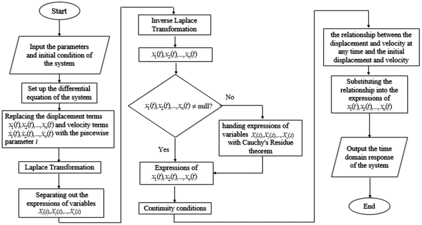
According to the theoretical descriptions above, pseudocode and flowchart of the Piecewise-Laplace method are shown in Figures 1 and 2.

Figure 1.

Pseudocode of the Piecewise-Laplace method.

Figure 2.

Flowchart of the Piecewise-Laplace method.

To demonstrate accuracy and reliability of the Piecewise-Laplace method for solving coupling oscillation system, three kinds of two-degree freedom systems are considered.

Solution of SCS

To explore the Piecewise-Laplace (PL) method for solving the coupling dynamics system, only a simple stiffness coupling system (SCS) is first shown in Figure 3, where $m_n(n=1,2)$ is the mass of the vibrator, $k_n(n=1,2)$ represents the stiffness coefficient of the spring and $x_n(n=1,2)$ denotes the displacement response of the vibrator. By applying an initial velocity and initial displacement to the vibrator, the response of the vibrator changes with time.

Figure 3.

The physical model of SCS.

According to the physical model, the following differential equation can be established

$$\begin{array}{c}{m}_1{x″}_1+k_1(x_1-x_2)=0\hfill \\ m_2{x″}_2+k_1(x_2-x_1)+k_2{x}_2=0\hfill \end{array}$$

(23)

The simplified form of equation (23) can be expressed as

$$\begin{array}{c}{x″}_1+{\omega }_{1,1}^2(x_1-x_2)=0\hfill \\ {x″}_2+{\omega }_{1,2}^2(x_2-x_1)+{\omega }_{2,2}^2{x}_2=0\hfill \end{array}$$

(24)

where ${\omega }_{1,1}=\sqrt{k_1/m_1},{\omega }_{1,2}=\sqrt{k_1/m_2},{\omega }_{2,2}=\sqrt{k_2/m_2}$ . The initial value of the system can be assumed by

$$\begin{array}{c}{x}_1(0)=d_{1,0},{x\prime }_1(0)=v_{1,0}\hfill \\ x_2(0)=d_{2,0},{x\prime }_2(0)=v_{2,0}\hfill \end{array}$$

(25)

Subsequently, the piecewise constant method should be employed to rearrange the continuous equation (24) as piecewise constant system. Replace terms $x_1(t)$ and $x_2(t)$ with piecewise constant functions $x_{1,i}(\frac{i}{N})$ and $x_{2,i}(\frac{i}{N})$ at arbitrary intervals of $i/N⩽t<(i+1)/N$ (i = [Nt]), and so equation (24) can expressed as

$$\begin{array}{c}{x″}_{1,i}+{\omega }_{1,1}^2{x}_{1,i}\left(\frac{i}{N}\right)-{\omega }_{1,1}^2{x}_{2,i}\left(\frac{i}{N}\right)=0\hfill \\ {x″}_{2,i}+{\omega }_{1,2}^2{x}_{2,i}\left(\frac{i}{N}\right)-{\omega }_{1,2}^2{x}_{1,i}\left(\frac{i}{N}\right)+{\omega }_{2,2}^2{x}_{2,i}\left(\frac{i}{N}\right)=0\hfill \end{array}$$

(26)

In this case, the local initial conditions in equation (25) can be transformed into the following form

$$\begin{array}{c}{x}_{1,i}\left(\frac{i}{N}\right)=d_{1,i},{x\prime }_{1,i}\left(\frac{i}{N}\right)=v_{1,i}\hfill \\ x_{2,i}\left(\frac{i}{N}\right)=d_{2,i},{x\prime }_{2,i}\left(\frac{i}{N}\right)=v_{2,i}\hfill \end{array}$$

(27)

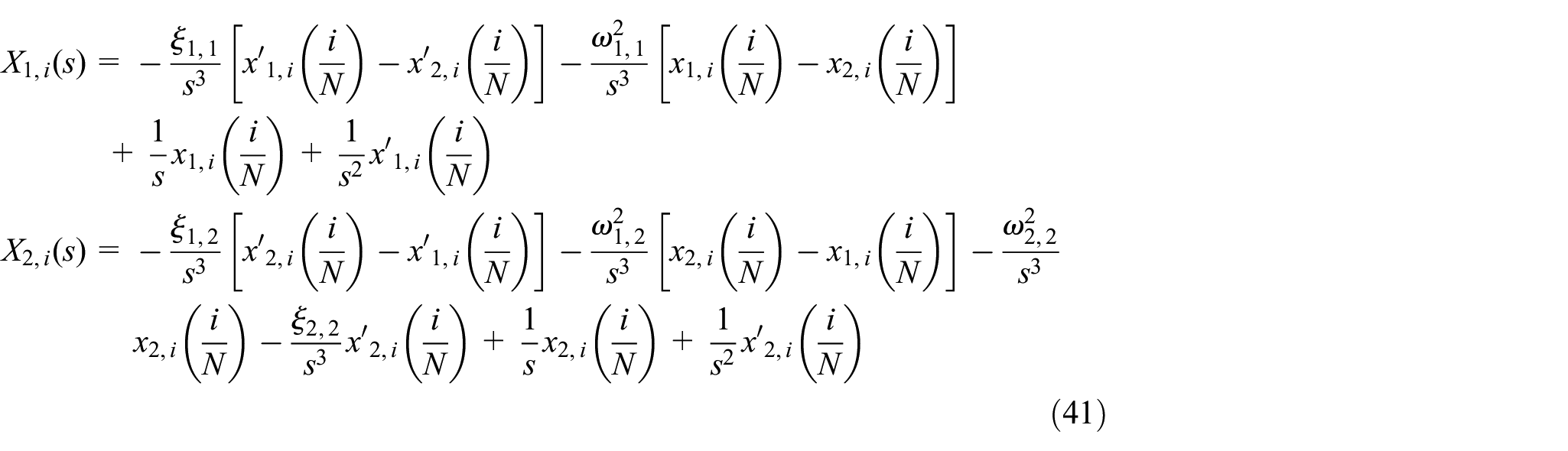
It can be found from equation (26), the piecewise style is coupled with respect to $x_{1,i}$ and $x_{2,i}$ . Therefore, the Laplace transformation can be used to separate the coupling variables, and the plural form of equation (26) in the interval $i/N⩽t<(i+1)/N$ is calculated as

$$\begin{array}{c}{s}^2{X}_{1,i}(s)-s{x}_{1,i}\left(\frac{i}{N}\right)-{x\prime }_{1,i}\left(\frac{i}{N}\right)+\frac{{\omega }_{1,1}^2}{s}{x}_{1,i}\left(\frac{i}{N}\right)-\frac{{\omega }_{1,1}^2}{s}{x}_{2,i}\left(\frac{i}{N}\right)=0\hfill \\ s^2{X}_{2,i}(s)-s{x}_{2,i}\left(\frac{i}{N}\right)-{x\prime }_{2,i}\left(\frac{i}{N}\right)+\frac{{\omega }_{1,2}^2}{s}{x}_{2,i}\left(\frac{i}{N}\right)-\frac{{\omega }_{1,2}^2}{s}{x}_{1,i}\left(\frac{i}{N}\right)+\frac{{\omega }_{2,2}^2}{s}{x}_{2,i}\left(\frac{i}{N}\right)=0\hfill \end{array}$$

(28)

Then, $X_{1,i}(s)$ and $X_{2,i}(s)$ can be expressed as

$$\begin{array}{c}{X}_{1,i}(s)=\frac{1}{s}{x}_{1,i}\left(\frac{i}{N}\right)+\frac{1}{s^2}{x\prime }_{1,i}\left(\frac{i}{N}\right)-\frac{{\omega }_{1,1}^2}{s^3}{x}_{1,i}\left(\frac{i}{N}\right)+\frac{{\omega }_{1,1}^2}{s^3}{x}_{2,i}\left(\frac{i}{N}\right)\hfill \\ X_{2,i}(s)=\frac{1}{s}{x}_{2,i}\left(\frac{i}{N}\right)+\frac{1}{s^2}{x\prime }_{2,i}\left(\frac{i}{N}\right)-\frac{{\omega }_{1,2}^2}{s^3}{x}_{2,i}\left(\frac{i}{N}\right)+\frac{{\omega }_{1,2}^2}{s^3}{x}_{1,i}\left(\frac{i}{N}\right)-\frac{{\omega }_{2,2}^2}{s^3}{x}_{2,i}\left(\frac{i}{N}\right)\hfill \end{array}$$

(29)

In this situation, $X_{1,i}(s)$ and $X_{2,i}(s)$ are the plural form of $x_{1,i}(t)$ and $x_{2,i}(t)$ in interval $i/N⩽t<(i+1)/N$ , respectively. Through using the reverse Laplace transformation, the expressions of $x_{1,i}(t)$ and $x_{2,i}(t)$ can be obtained by the replacement of i with [Nt]

$$\begin{array}{c}{x}_{1,i}(t)={\mathbf{A}}_1{\mathbf{v}}_i\hfill \\ x_{2,i}(t)={\mathbf{A}}_2{\mathbf{v}}_i\hfill \end{array}$$

(30)

where

$$\begin{array}{c}{\mathbf{A}}_1=\left[1-\frac{1}{2}{\omega }_{1,1}^2{\left(t-\frac{[Nt]}{N}\right)}^2,t-\frac{[Nt]}{N},\frac{1}{2}{\omega }_{1,1}^2{\left(t-\frac{[Nt]}{N}\right)}^2,0\right],{\mathbf{A}}_2=\left[\frac{1}{2}{\omega }_{1,2}^2{\left(t-\frac{[Nt]}{N}\right)}^2,0,1-\frac{1}{2}{\omega }_{1,2}^2{\left(t-\frac{[Nt]}{N}\right)}^2-\frac{1}{2}{\omega }_{2,2}^2{\left(t-\frac{[Nt]}{N}\right)}^2,t-\frac{[Nt]}{N}\right]\\ {\mathbf{v}}_i={[d_{1,i},v_{1,i},d_{2,i},v_{2,i}]}^T\end{array}$$

Therefore, the velocities $x{\prime }_{1,i}(t)$ and $x{\prime }_{2,i}(t)$ should be rewritten as follows

$$\begin{array}{c}{x\prime }_{1,i}(t)=\frac{\partial {\mathbf{A}}_1}{\partial t}{\mathbf{v}}_i\hfill \\ {x\prime }_{2,i}(t)=\frac{\partial {\mathbf{A}}_2}{\partial t}{\mathbf{v}}_i\hfill \end{array}$$

(31)

As mentioned previously, the displacements $(x_{1,i}(t),x_{2,i}(t))$ and the velocities $(x{\prime }_{1,i}(t),x{\prime }_{2,i}(t))$ are continuous in $t\in [0,+\infty )$ , which is physically implied that there is no jump (break) or discontinuity in the displacement and velocity over $t\in [0,+\infty )$ . Thus, the displacement and velocity in two adjacent points must satisfy the following continuity conditions

$$\begin{array}{c}{x}_{1,i}\left(\frac{i}{N}\right)=x_{1,i-1}\left(\frac{i}{N}\right),{x\prime }_{1,i}\left(\frac{i}{N}\right)={x\prime }_{1,i-1}\left(\frac{i}{N}\right)\hfill \\ x_{2,i}\left(\frac{i}{N}\right)=x_{2,i-1}\left(\frac{i}{N}\right),{x\prime }_{2,i}\left(\frac{i}{N}\right)={x\prime }_{2,i-1}\left(\frac{i}{N}\right)\hfill \end{array}$$

(32)

According to the continuity conditions in equation (32), the relation of displacement and velocity between the two adjacent truncation points can be represented as

$${\mathbf{v}}_i=\mathbf{p}{\mathbf{v}}_{i-1}$$

(33)

where ${\mathbf{v}}_i=[d_{1,i},v_{1,i},d_{2,i},v_{2,i}{]}^T,{\mathbf{v}}_{i-1}=[d_{1,i-1},v_{1,i-1},d_{2,i-1},v_{2,i-1}{]}^T,\mathbf{p}=[p_{\mathrm{ij}}{]}_{4\times 4}(i=1,\cdots ,4,j=1,\cdots ,4),$ the elements of the matrix $\mathbf{p}$ are shown as follows

$$\begin{array}{c}{p}_{11}=1-\frac{{\omega }_{1,1}^2}{2N^2},p_{12}=\frac{1}{N},p_{13}=\frac{{\omega }_{1,1}^2}{2N^2},p_{14}=0,p_{21}=-\frac{{\omega }_{1,1}^2}{N},p_{22}=1,p_{23}=\frac{{\omega }_{1,1}^2}{N},p_{24}=0\hfill \\ p_{31}=\frac{{\omega }_{1,2}^2}{2N^2},p_{32}=0,p_{33}=1-\frac{{\omega }_{1,2}^2}{2N^2}-\frac{{\omega }_{2,2}^2}{2N^2},p_{34}=\frac{1}{N},p_{41}=\frac{{\omega }_{1,2}^2}{N},p_{42}=0,p_{43}=-\frac{{\omega }_{1,2}^2}{N}-\frac{{\omega }_{2,2}^2}{N},p_{44}=1\hfill \end{array}$$

(34)

In light of equation (33), ${\mathbf{v}}_i$ can be expressed via initial condition ${\mathbf{v}}_0$ with iterative computations of i times, that is

$${\mathbf{v}}_i={\mathbf{p}}^i{\mathbf{v}}_0$$

(35)

where ${\mathbf{v}}_0=[d_{1,0},v_{1,0},d_{2,0},v_{2,0}{]}^T$ .

When the initial condition ${\mathbf{v}}_0$ is determined, the displacement and velocity of the system at any time can be calculated by utilizing equation (35). The semi-analytical solution of the system in i-th interval can be rewritten as the style of piecewise constant, that is

$$\begin{array}{c}{x}_{1,i}(t)={\mathbf{A}}_1{\mathbf{p}}^{[\mathrm{Nt}]}{\mathbf{v}}_0\hfill \\ x_{2,i}(t)={\mathbf{A}}_2{\mathbf{p}}^{[\mathrm{Nt}]}{\mathbf{v}}_0\hfill \end{array}$$

(36)

Solution of SDCS

In actual engineering, damping is usually existed in coupling dynamics system. Therefore, a dynamic system coupled with the terms of stiffness and damping (SDCS) is considered, as shown in Figure 4, where $m_n(n=1,2)$ is the mass of the vibrator, $k_n(n=1,2)$ represents the stiffness coefficient of the spring, $c_n(n=1,2)$ is the damping coefficient of the damper and $x_n(n=1,2)$ denotes the displacement response of the vibrator. Likewise, give the vibrator an initial velocity and initial displacement, and the analytical expression of the response of the vibrator can be obtained by the PL method.

Through this model, the following equation can be obtained

$$\begin{array}{c}{m}_1{x″}_1+c_1({x\prime }_1-{x\prime }_2)+k_1(x_1-x_2)=0\hfill \\ m_2{x″}_2+c_1({x\prime }_2-{x\prime }_1)+k_1(x_2-x_1)+k_2{x}_2+c_2{x\prime }_2=0\hfill \end{array}$$

(37)

Figure 4.

The physical model of SDCS.

The simplified form of equation (37) can be expressed as

$$\begin{array}{c}{x″}_1+{\xi }_{1,1}({x\prime }_1-{x\prime }_2)+{\omega }_{1,1}^2(x_1-x_2)=0\hfill \\ {x″}_2+{\xi }_{1,2}({x\prime }_2-{x\prime }_1)+{\omega }_{1,2}^2(x_2-x_1)+{\omega }_{2,2}^2{x}_2+{\xi }_{2,2}{x\prime }_2=0\hfill \end{array}$$

(38)

where ${\omega }_{1,1}=\sqrt{k_1/m_1},{\omega }_{1,2}=\sqrt{k_1/m_2},{\omega }_{2,2}=\sqrt{k_2/m_2},{\xi }_{1,1}=c_1/m_1,{\xi }_{1,2}=c_1/m_2,{\xi }_{2,2}=c_2/m_2.$

In arbitrary interval $i/N⩽t<(i+1)/N$ , equation (38) can be rearranged as a style of piecewise constant. Replace terms $x_1(t)$ , $x{\prime }_1(t)$ , $x_2(t)$ and $x{\prime }_2(t)$ with piecewise constant functions $x_{1,i}(\frac{i}{N})$ , $x{\prime }_{1,i}(\frac{i}{N})$ , $x_{2,i}(\frac{i}{N})$ and $x{\prime }_{2,i}(\frac{i}{N})$ , and so equation (38) can expressed as

$$\begin{array}{c}{x″}_1+{\xi }_{1,1}[{x\prime }_{1,i}\left(\frac{i}{N}\right)-{x\prime }_{2,i}\left(\frac{i}{N}\right)]+{\omega }_{1,1}^2[x_{1,i}\left(\frac{i}{N}\right)-x_{2,i}\left(\frac{i}{N}\right)]=0\hfill \\ {x″}_2+{\xi }_{1,2}[{x\prime }_{2,i}\left(\frac{i}{N}\right)-{x\prime }_{1,i}\left(\frac{i}{N}\right)]+{\omega }_{1,2}^2[x_{2,i}\left(\frac{i}{N}\right)-x_{1,i}\left(\frac{i}{N}\right)]\hfill \\ \multicolumn{1}{c}{+{\omega }_{2,2}^2{x}_{2,i}\left(\frac{i}{N}\right)+{\xi }_{2,2}{x\prime }_{2,i}\left(\frac{i}{N}\right)=0}\end{array}$$

(39)

The Laplace transformation can be used to separate the coupling variables, and the transformed plural form of equation (39) in the interval $i/N⩽t<(i+1)/N$ is calculated as

$$\begin{array}{c}{s}^2{X}_{1,i}(s)-s{x}_{1,i}\left(\frac{i}{N}\right)-{x\prime }_{1,i}\left(\frac{i}{N}\right)=-\frac{{\xi }_{1,1}}{s}[{x\prime }_{1,i}\left(\frac{i}{N}\right)-{x\prime }_{2,i}\left(\frac{i}{N}\right)]\hfill \\ \multicolumn{1}{c}{-\frac{{\omega }_{1,1}^2}{s}[x_{1,i}\left(\frac{i}{N}\right)-x_{2,i}\left(\frac{i}{N}\right)]}\\ s^2{X}_{2,i}(s)-s{x}_{2,i}\left(\frac{i}{N}\right)-{x\prime }_{2,i}\left(\frac{i}{N}\right)=-\frac{{\xi }_{1,2}}{s}[{x\prime }_{2,i}\left(\frac{i}{N}\right)-{x\prime }_{1,i}\left(\frac{i}{N}\right)]\hfill \\ \multicolumn{1}{c}{-\frac{{\omega }_{1,2}^2}{s}[x_{2,i}\left(\frac{i}{N}\right)-x_{1,i}\left(\frac{i}{N}\right)]-\frac{{\omega }_{2,2}^2}{s}{x}_{2,i}\left(\frac{i}{N}\right)-\frac{{\xi }_{2,2}}{s}{x\prime }_{2,i}\left(\frac{i}{N}\right)}\end{array}$$

(40)

Then, $X_{1,i}(s)$ and $X_{2,i}(s)$ can be expressed as

$$\begin{array}{c}{X}_{1,i}(s)=-\frac{{\xi }_{1,1}}{s^3}[{x\prime }_{1,i}\left(\frac{i}{N}\right)-{x\prime }_{2,i}\left(\frac{i}{N}\right)]-\frac{{\omega }_{1,1}^2}{s^3}[x_{1,i}\left(\frac{i}{N}\right)-x_{2,i}\left(\frac{i}{N}\right)]\hfill \\ \multicolumn{1}{c}{+\frac{1}{s}{x}_{1,i}\left(\frac{i}{N}\right)+\frac{1}{s^2}{x\prime }_{1,i}\left(\frac{i}{N}\right)}\\ X_{2,i}(s)=-\frac{{\xi }_{1,2}}{s^3}[{x\prime }_{2,i}\left(\frac{i}{N}\right)-{x\prime }_{1,i}\left(\frac{i}{N}\right)]-\frac{{\omega }_{1,2}^2}{s^3}[x_{2,i}\left(\frac{i}{N}\right)-x_{1,i}\left(\frac{i}{N}\right)]-\frac{{\omega }_{2,2}^2}{s^3}\hfill \\ \multicolumn{1}{c}{x_{2,i}\left(\frac{i}{N}\right)-\frac{{\xi }_{2,2}}{s^3}{x\prime }_{2,i}\left(\frac{i}{N}\right)+\frac{1}{s}{x}_{2,i}\left(\frac{i}{N}\right)+\frac{1}{s^2}{x\prime }_{2,i}\left(\frac{i}{N}\right)}\end{array}$$

(41)

Through using the reverse Laplace transformation, the expressions of $x_{1,i}(t)$ and $x_{2,i}(t)$ can be obtained by the replacement of i with [Nt]

$$\begin{array}{c}{x}_{1,i}(t)={\mathbf{B}}_1{\mathbf{v}}_i\hfill \\ x_{2,i}(t)={\mathbf{B}}_2{\mathbf{v}}_i\hfill \end{array}$$

(42)

where

$$\begin{array}{c}{\mathbf{v}}_i={[d_{1,i},v_{1,i},d_{2,i},v_{2,i}]}^T,\hfill \\ \multicolumn{1}{c}{{\mathbf{B}}_1=[1-\frac{1}{2}{\omega }_{1,1}^2{(t-\frac{[\mathrm{Nt}]}{N})}^2,t-\frac{[\mathrm{Nt}]}{N}-\frac{1}{2}{\xi }_{1,1}{(t-\frac{[\mathrm{Nt}]}{N})}^2,\frac{1}{2}{\omega }_{1,1}^2{(t-\frac{[\mathrm{Nt}]}{N})}^2,\frac{1}{2}{\xi }_{1,1}{(t-\frac{[\mathrm{Nt}]}{N})}^2]}\\ {\mathbf{B}}_2=[\frac{1}{2}{\omega }_{1,2}^2{(t-\frac{[\mathrm{Nt}]}{N})}^2,\frac{1}{2}{\xi }_{1,2}{(t-\frac{[\mathrm{Nt}]}{N})}^2,1-\frac{1}{2}{\omega }_{1,2}^2{(t-\frac{[\mathrm{Nt}]}{N})}^2-\frac{1}{2}{\omega }_{2,2}^2{(t-\frac{[\mathrm{Nt}]}{N})}^2,(t-\frac{[\mathrm{Nt}]}{N})-\frac{1}{2}{\xi }_{1,2}{(t-\frac{[\mathrm{Nt}]}{N})}^2-\frac{1}{2}{\xi }_{2,2}{(t-\frac{[\mathrm{Nt}]}{N})}^2]\hfill \end{array}$$

Therefore, the velocities $x{\prime }_{1,i}(t)$ and $x{\prime }_{2,i}(t)$ should be rewritten as follows

$$\begin{array}{c}{x\prime }_{1,i}=\frac{\partial {\mathbf{B}}_1}{\partial t}{\mathbf{v}}_i\hfill \\ {x\prime }_{2,i}=\frac{\partial {\mathbf{B}}_2}{\partial t}{\mathbf{v}}_i\hfill \end{array}$$

(43)

In the light of the continuity conditions in equation (32), the relation of displacement and velocity between the two adjacent truncation points can be represented as

$${\mathbf{v}}_i=\mathbf{q}{\mathbf{v}}_{i-1}$$

(44)

where ${\mathbf{v}}_{i-1}=[d_{1,i-1},v_{1,i-1},d_{2,i-1},v_{2,i-1}{]}^T,\mathbf{q}=[q_{\mathrm{ij}}{]}_{4\times 4}(i=1,\cdots ,4,j=1,\cdots ,4),$ the elements in matrix $\mathbf{q}$ are given by

$$\begin{array}{c}{q}_{11}=1-\frac{{\omega }_{1,1}^2}{2N^2},q_{12}=\frac{1}{N}-\frac{{\xi }_{1,1}}{2N^2},q_{13}=\frac{{\omega }_{1,1}^2}{2N^2},q_{14}=\frac{{\xi }_{1,1}}{2N^2}\hfill \\ q_{21}=-\frac{{\omega }_{1,1}^2}{N},q_{22}=1-\frac{{\xi }_{1,1}}{N},q_{23}=\frac{{\omega }_{1,1}^2}{N},q_{24}=\frac{{\xi }_{1,1}}{N}\hfill \\ q_{31}=\frac{{\omega }_{1,2}^2}{2N^2},q_{32}=\frac{{\xi }_{1,2}}{2N^2},q_{33}=1-\frac{{\omega }_{1,2}^2}{2N^2}-\frac{{\omega }_{2,2}^2}{2N^2},q_{34}=\frac{1}{N}-\frac{{\xi }_{1,2}}{2N^2}-\frac{{\xi }_{2,2}}{2N^2}\hfill \\ q_{41}=\frac{{\omega }_{1,2}^2}{N},q_{42}=\frac{{\xi }_{1,2}}{N},q_{43}=-\frac{{\omega }_{1,2}^2}{N}-\frac{{\omega }_{2,2}^2}{N},q_{44}=1-\frac{{\xi }_{1,2}}{N}-\frac{{\xi }_{2,2}}{N}\hfill \end{array}$$

(45)

According to the equation (44), ${\mathbf{v}}_i$ can be expressed via initial condition ${\mathbf{v}}_0$ with iterative computations of i times, that is

$${\mathbf{v}}_i={\mathbf{q}}^i{\mathbf{v}}_0$$

(46)

where ${\mathbf{v}}_0=[d_{1,0},v_{1,0},d_{2,0},v_{2,0}{]}^T.$

When initial condition ${\mathbf{v}}_0$ is determined, the displacement and velocity of the system at any time can be calculated by utilizing equation (46). The semi-analytical solution of the system in i-th interval can be rewritten as the style of piecewise constant, that is

$$\begin{array}{c}{x}_{1,i}(t)={\mathbf{B}}_1{\mathbf{q}}^{[\mathrm{Nt}]}{\mathbf{v}}_0\hfill \\ x_{2,i}(t)={\mathbf{B}}_2{\mathbf{q}}^{[\mathrm{Nt}]}{\mathbf{v}}_0\hfill \end{array}$$

(47)

Solution of SDCSF

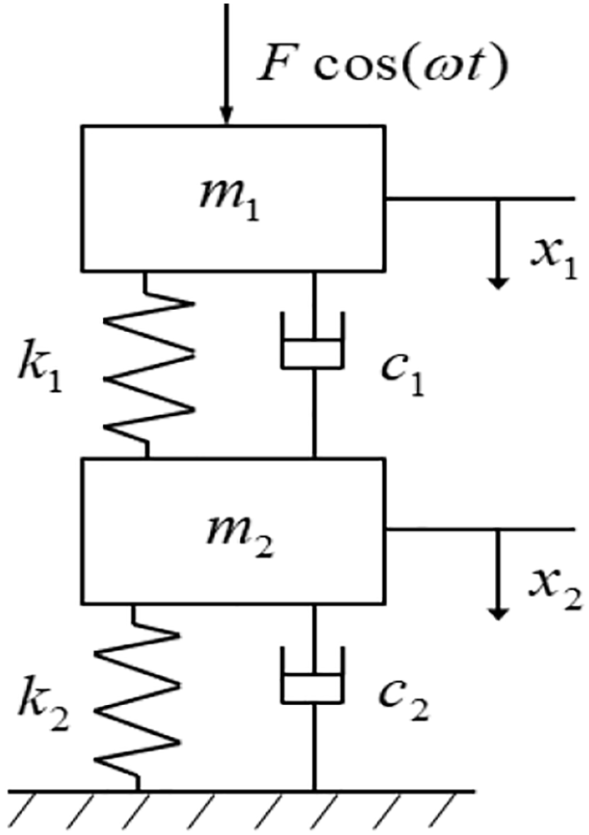
In practical engineering, the stiffness and damping coupling system is encountered external excitation. Consider a cosine force related to time t acted in the system (SDCSF) as shown in Figure 5, where $m_n(n=1,2)$ is the mass of the vibrator, $k_n(n=1,2)$ represents the stiffness coefficient of the spring, $c_n(n=1,2)$ is the damping coefficient of the damper, $F$ is the magnitude of the cosine force, $\omega$ represents the frequency of the cosine force and $x_n(n=1,2)$ denotes the displacement response of the vibrator. When the external excitation acting on the vibrator changes periodically with time, the vibrator will respond accordingly.

Figure 5.

The physical model of SDCSF.

According to the physical model, the following equation is established

$$\begin{array}{c}{m}_1{x″}_1+c_1({x\prime }_1-{x\prime }_2)+k_1(x_1-x_2)=F\cos (\omega t)\hfill \\ m_2{x″}_2+c_1({x\prime }_2-{x\prime }_1)+k_1(x_2-x_1)+k_2{x}_2+c_2{x\prime }_2=0\hfill \end{array}$$

(48)

The simplified form of equation (48) can be expressed as

$$\begin{array}{c}{x″}_1+{\xi }_{1,1}({x\prime }_1-{x\prime }_2)+{\omega }_{1,1}^2(x_1-x_2)=a\cos (\omega t)\hfill \\ {x″}_2+{\xi }_{1,2}({x\prime }_2-{x\prime }_1)+{\omega }_{1,2}^2(x_2-x_1)+{\omega }_{2,2}^2{x}_2+{\xi }_{2,2}{x\prime }_2=0\hfill \end{array}$$

(49)

where $a=F/m_1,{\omega }_{1,1}=\sqrt{k_1/m_1},{\omega }_{1,2}=\sqrt{k_1/m_2},{\omega }_{2,2}=\sqrt{k_2/m_2},{\xi }_{1,1}=c_1/m_1,{\xi }_{1,2}=c_1/m_2,{\xi }_{2,2}=c_2/m_2$ .

At time interval $i/N⩽t<(i+1)/N$ , the piecewise constant method is employed to rearrange equation (49) as the style of piecewise constant. Replace terms $x{\prime }_1(t)$ , $x{\prime }_2(t)$ and $a\cos (\omega t)$ with the piecewise constant functions $x{\prime }_{1,i}(\frac{i}{N})$ , $x{\prime }_{2,i}(\frac{i}{N})$ and $a\cos (\omega \frac{i}{N})$ , respectively. Equation (49) can expressed as

$$\begin{array}{c}{x″}_1+{\xi }_{1,1}[{x\prime }_{1,i}\left(\frac{i}{N}\right)-{x\prime }_{2,i}\left(\frac{i}{N}\right)]+{\omega }_{1,1}^2(x_1-x_2)=a\cos \left(\omega \frac{i}{N}\right)\hfill \\ {x″}_2+{\omega }_{1,2}^2(x_2-x_1)+{\xi }_{1,2}[{x\prime }_{2,i}\left(\frac{i}{N}\right)-{x\prime }_{1,i}\left(\frac{i}{N}\right)]+{\omega }_{2,2}^2{x}_2+{\xi }_{2,2}{x\prime }_{2,i}\left(\frac{i}{N}\right)=0\hfill \end{array}$$

(50)

The Laplace transformation can be used to separate the coupling variables, and the plural form of equation (50) in the interval $i/N⩽t<(i+1)/N$ is calculated as

$$\begin{array}{c}{s}^2{X}_{1,i}(s)+{\omega }_{1,1}^2[X_{1,i}(s)-X_{2,i}(s)]=\hfill \\ \multicolumn{1}{c}{a\cos \left(\omega \frac{i}{N}\right)-{\xi }_{1,1}[{x\prime }_{1,i}\left(\frac{i}{N}\right)-{x\prime }_{2,i}\left(\frac{i}{N}\right)]+s{x}_{1,i}\left(\frac{i}{N}\right)+{x\prime }_{1,i}\left(\frac{i}{N}\right)}\\ s^2{X}_{2,i}(s)+{\omega }_{1,2}^2[X_{2,i}(s)-X_{1,i}(s)]+{\omega }_{2,2}^2{X}_{2,i}(s)=\hfill \\ \multicolumn{1}{c}{-{\xi }_{1,2}[{x\prime }_{2,i}\left(\frac{i}{N}\right)-{x\prime }_{1,i}\left(\frac{i}{N}\right)]-{\xi }_{2,2}{x\prime }_{2,i}\left(\frac{i}{N}\right)+s{x}_{2,i}\left(\frac{i}{N}\right)+{x\prime }_{2,i}\left(\frac{i}{N}\right).}\end{array}$$

(51)

Then, $X_{1,i}(s)$ and $X_{2,i}(s)$ can be decoupled and expressed as

$$\begin{array}{c}\multicolumn{1}{c}{X_{1,i}(s)=\frac{\mathrm{sW}}{\mathrm{QW}-{\omega }_{1,1}^2{\omega }_{1,2}^2}{x}_{1,i}\left(\frac{i}{N}\right)+[\frac{W}{\mathrm{QW}-{\omega }_{1,1}^2{\omega }_{1,2}^2}+\frac{{\xi }_{1,2}{\omega }_{1,1}^2-{\xi }_{1,1}W}{s(\mathrm{QW}-{\omega }_{1,1}^2{\omega }_{1,2}^2)}]{x\prime }_{1,i}\left(\frac{i}{N}\right)}\\ \multicolumn{1}{c}{+\frac{s{\omega }_{1,1}^2}{\mathrm{QW}-{\omega }_{1,1}^2{\omega }_{1,2}^2}{x}_{2,i}\left(\frac{i}{N}\right)+[\frac{{\xi }_{1,1}W-{\xi }_{1,2}{\omega }_{1,1}^2-{\xi }_{2,2}{\omega }_{1,1}^2}{s(\mathrm{QW}-{\omega }_{1,1}^2{\omega }_{1,2}^2)}+\frac{{\omega }_{1,1}^2}{\mathrm{QW}-{\omega }_{1,1}^2{\omega }_{1,2}^2}]{x\prime }_{2,i}\left(\frac{i}{N}\right)}\\ \multicolumn{1}{c}{+\frac{W}{s(\mathrm{QW}-{\omega }_{1,1}^2{\omega }_{1,2}^2)}a\cos \left(\omega \frac{i}{N}\right)}\\ \multicolumn{1}{c}{X_{2,i}(s)=\frac{2s{\omega }_{1,2}^2}{\mathrm{QW}-{\omega }_{1,1}^2{\omega }_{1,2}^2}{x}_{1,i}\left(\frac{i}{N}\right)}\\ \multicolumn{1}{c}{+[\frac{{\xi }_{1,2}}{\mathrm{sW}}+\frac{{\omega }_{1,2}^2}{\mathrm{QW}-{\omega }_{1,1}^2{\omega }_{1,2}^2}-\frac{{\xi }_{1,1}{\omega }_{1,2}^2}{s(\mathrm{QW}-{\omega }_{1,1}^2{\omega }_{1,2}^2)}+\frac{{\xi }_{1,2}{\omega }_{1,1}^2{\omega }_{1,2}^2}{\mathrm{sW}(\mathrm{QW}-{\omega }_{1,1}^2{\omega }_{1,2}^2)}]{x\prime }_{1,i}\left(\frac{i}{N}\right)}\\ \multicolumn{1}{c}{+[\frac{1}{W}-\frac{{\xi }_{1,2}+{\xi }_{2,2}}{\mathrm{sW}}+\frac{{\xi }_{1,1}{\omega }_{1,2}^2}{s(\mathrm{QW}-{\omega }_{1,1}^2{\omega }_{1,2}^2)}+\frac{{\omega }_{1,1}^2{\omega }_{1,2}^2}{W(\mathrm{QW}-{\omega }_{1,1}^2{\omega }_{1,2}^2)}-\frac{{\xi }_{1,2}{\omega }_{1,1}^2{\omega }_{1,2}^2+{\xi }_{2,2}{\omega }_{1,1}^2{\omega }_{1,2}^2}{\mathrm{sW}(\mathrm{QW}-{\omega }_{1,1}^2{\omega }_{1,2}^2)}]{x\prime }_{2,i}\left(\frac{i}{N}\right)}\\ \multicolumn{1}{c}{+[\frac{s}{W}+\frac{s{\omega }_{1,1}^2{\omega }_{1,2}^2}{W(\mathrm{QW}-{\omega }_{1,1}^2{\omega }_{1,2}^2)}]x_{2,i}\left(\frac{i}{N}\right)+\frac{{\omega }_{1,2}^2}{s(\mathrm{QW}-{\omega }_{1,1}^2{\omega }_{1,2}^2)}a\cos \left(\omega \frac{i}{N}\right)}\end{array}$$

(52)

where $Q=s^2+{\omega }_{1,1}^2,W=s^2+{\omega }_{1,2}^2+{\omega }_{2,2}^2$ .

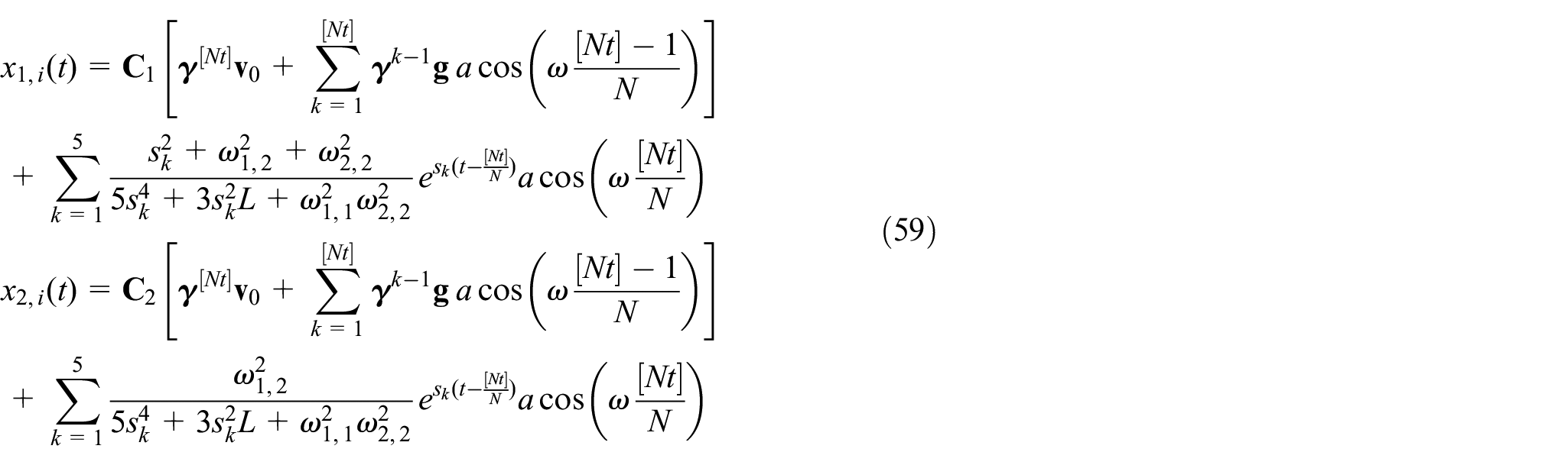
It is difficult to transform plural solution above into time-domain solution with the general reverse Laplace-transform. However, Through Theorem 5 in equation (22), the expressions of $x_{1,i}(t)$ and $x_{2,i}(t)$ can be obtained by the replacement of i with [Nt]

$$\begin{array}{c}{x}_{1,i}(t)={\mathbf{C}}_1{\mathbf{v}}_i+\sum _{k=1}^5\frac{s_k^2+{\omega }_{1,2}^2+{\omega }_{2,2}^2}{5s_k^4+3s_k^{2}L+{\omega }_{1,1}^2{\omega }_{2,2}^2}{e}^{s_k(t-\frac{i}{N})}a\cos \left(\omega \frac{i}{N}\right)\hfill \\ x_{2,i}(t)={\mathbf{C}}_2{\mathbf{v}}_i+\sum _{k=1}^5\frac{{\omega }_{1,2}^2}{5s_k^4+3s_k^{2}L+{\omega }_{1,1}^2{\omega }_{2,2}^2}{e}^{s_k(t-\frac{i}{N})}a\cos \left(\omega \frac{i}{N}\right)\hfill \end{array}$$

(53)

where ${\mathbf{v}}_i=[d_{1,i},v_{1,i},d_{2,i},v_{2,i}{]}^T,L={\omega }_{1,1}^2+{\omega }_{1,2}^2+{\omega }_{2,2}^2,$

$$\begin{array}{c}\multicolumn{1}{c}{{\mathbf{C}}_1={\left[\begin{array}{c}\sum _{k=1}^4\frac{s_k^2+{\omega }_{1,2}^2+{\omega }_{2,2}^2}{4s_k^2+2L}{e}^{s_k(t-\frac{i}{N})}\hfill \\ \multicolumn{1}{c}{\sum _{k=1}^4\frac{s_k^2+{\omega }_{1,2}^2+{\omega }_{2,2}^2}{4s_k^3+2s_{k}L}{e}^{s_k(t-\frac{i}{N})}+\sum _{k=1}^5\frac{{\xi }_{1,2}{\omega }_{1,1}^2-{\xi }_{1,1}(s_k^2+{\omega }_{1,2}^2+{\omega }_{2,2}^2)}{5s_k^4+3s_k^{2}L+{\omega }_{1,1}^2{\omega }_{2,2}^2}{e}^{s_k(t-\frac{i}{N})}}\\ \multicolumn{1}{c}{\sum _{k=1}^4\frac{{\omega }_{1,1}^2}{4s_k^2+2L}{e}^{s_k(t-\frac{i}{N})}}\\ \multicolumn{1}{c}{\sum _{k=1}^4\frac{{\omega }_{1,1}^2}{4s_k^3+2s_{k}L}{e}^{s_k(t-\frac{i}{N})}+\sum _{k=1}^5\frac{-{\xi }_{2,2}{\omega }_{1,1}^2-{\xi }_{1,2}{\omega }_{1,1}^2+{\xi }_{1,1}(s_k^2+{\omega }_{1,2}^2+{\omega }_{2,2}^2)}{5s_k^4+3s_k^{2}L+{\omega }_{1,1}^2{\omega }_{2,2}^2}{e}^{s_k(t-\frac{i}{N})}}\end{array}\right]}^{\mathrm{T}}}\\ {\mathbf{C}}_2={\left[\begin{array}{c}\sum _{k=1}^4\frac{{\omega }_{1,2}^2}{2s_k^2+L}{e}^{s_k(t-\frac{i}{N})}\hfill \\ \multicolumn{1}{c}{\sum _{k=5}^7\frac{{\xi }_{1,2}}{3s_k^2+{\omega }_{1,2}^2+{\omega }_{2,2}^2}{e}^{s_k(t-\frac{i}{N})}+\sum _{k=1}^4\frac{{\omega }_{1,2}^2}{4s_k^3+2s_{k}L}{e}^{s_k(t-\frac{i}{N})}-\sum _{k=1}^5\frac{{\xi }_{1,1}{\omega }_{1,2}^2}{5s_k^4+3s_k^{2}L+{\omega }_{1,1}^2{\omega }_{2,2}^2}{e}^{s_k(t-\frac{i}{N})}+\sum _{k=1}^7\frac{{\xi }_{1,2}{\omega }_{1,1}^2{\omega }_{1,2}^2}{\begin{array}{c}7s_k^6+5s_k^4({\omega }_{1,1}^2+2{\omega }_{1,2}^2+2{\omega }_{2,2}^2)+3s_k^2(2{\omega }_{1,1}^2{\omega }_{2,2}^2+{\omega }_{1,2}^4+{\omega }_{1,1}^2{\omega }_{1,2}^2\hfill \\ \multicolumn{1}{c}{+2{\omega }_{1,2}^2{\omega }_{2,2}^2+{\omega }_{2,2}^4)+({\omega }_{1,1}^2{\omega }_{1,2}^2{\omega }_{2,2}^2+{\omega }_{1,1}^2{\omega }_{2,2}^4)}\end{array}}{e}^{s_k(t-\frac{i}{N})}}\\ \multicolumn{1}{c}{\sum _{k=5}^7\frac{1}{2}{e}^{s_k(t-\frac{i}{N})}+\sum _{k=1}^4\frac{{\omega }_{1,2}^2}{\begin{array}{c}6s_k^4+4s_k^2({\omega }_{1,1}^2+2{\omega }_{1,2}^2+2{\omega }_{2,2}^2)\hfill \\ \multicolumn{1}{c}{+2(2{\omega }_{1,1}^2{\omega }_{2,2}^2+{\omega }_{1,2}^4+{\omega }_{1,1}^2{\omega }_{1,2}^2+2{\omega }_{1,2}^2{\omega }_{2,2}^2+{\omega }_{2,2}^4)}\end{array}}{e}^{s_k(t-\frac{i}{N})}+\sum _{k=6}^7\frac{{\omega }_{1,1}^2{\omega }_{1,2}^2}{\begin{array}{c}6s_k^4+4s_k^2({\omega }_{1,1}^2+2{\omega }_{1,2}^2+2{\omega }_{2,2}^2)\hfill \\ \multicolumn{1}{c}{+2(2{\omega }_{1,1}^2{\omega }_{2,2}^2+{\omega }_{1,2}^4+{\omega }_{1,1}^2{\omega }_{1,2}^2+2{\omega }_{1,2}^2{\omega }_{2,2}^2+{\omega }_{2,2}^4)}\end{array}}{e}^{s_k(t-\frac{i}{N})}}\\ \multicolumn{1}{c}{\begin{array}{c}\sum _{k=5}^7\frac{1}{2s_k}{e}^{s_k(t-\frac{i}{N})}-\sum _{k=5}^7\frac{{\xi }_{1,2}+{\xi }_{2,2}}{3s_k^2+{\omega }_{1,2}^2+{\omega }_{2,2}^2}{e}^{s_k(t-\frac{i}{N})}+\sum _{k=1}^5\frac{{\xi }_{1,1}{\omega }_{1,2}^2}{5s_k^4+3s_k^{2}L+{\omega }_{1,1}^2{\omega }_{2,2}^2}{e}^{s_k(t-\frac{i}{N})}+\sum _{k=1}^5\frac{{\xi }_{1,1}{\omega }_{1,2}^2}{\begin{array}{c}6s_k^5+4s_k^3({\omega }_{1,1}^2+2{\omega }_{1,2}^2+2{\omega }_{2,2}^2)\hfill \\ \multicolumn{1}{c}{+2s_k(2{\omega }_{1,1}^2{\omega }_{2,2}^2+{\omega }_{1,2}^4+{\omega }_{1,1}^2{\omega }_{1,2}^2+2{\omega }_{1,2}^2{\omega }_{2,2}^2+{\omega }_{2,2}^4)}\end{array}}{e}^{s_k(t-\frac{i}{N})}\hfill \\ \multicolumn{1}{c}{+\sum _{k=6}^7\frac{{\omega }_{1,1}^2{\omega }_{1,2}^2}{\begin{array}{c}6s_k^5+4s_k^3({\omega }_{1,1}^2+2{\omega }_{1,2}^2+2{\omega }_{2,2}^2)\hfill \\ \multicolumn{1}{c}{+2s_k(2{\omega }_{1,1}^2{\omega }_{2,2}^2+{\omega }_{1,2}^4+{\omega }_{1,1}^2{\omega }_{1,2}^2+2{\omega }_{1,2}^2{\omega }_{2,2}^2+{\omega }_{2,2}^4)}\end{array}}{e}^{s_k(t-\frac{i}{N})}-\sum _{k=1}^7\frac{{\xi }_{1,2}{\omega }_{1,1}^2{\omega }_{1,2}^2+{\xi }_{2,2}{\omega }_{1,1}^2{\omega }_{1,2}^2}{\begin{array}{c}7s_k^6+5s_k^4({\omega }_{1,1}^2+2{\omega }_{1,2}^2+2{\omega }_{2,2}^2)+3s_k^2(2{\omega }_{1,1}^2{\omega }_{2,2}^2+{\omega }_{1,2}^4+{\omega }_{1,1}^2{\omega }_{1,2}^2\hfill \\ \multicolumn{1}{c}{+2{\omega }_{1,2}^2{\omega }_{2,2}^2+{\omega }_{2,2}^4)+({\omega }_{1,1}^2{\omega }_{1,2}^2{\omega }_{2,2}^2+{\omega }_{1,1}^2{\omega }_{2,2}^4)}\end{array}}{e}^{s_k(t-\frac{i}{N})}}\end{array}}\end{array}\right]}^{\mathrm{T}}\hfill \end{array}$$

Therefore, the velocities $x{\prime }_{1,i}(t)$ and $x{\prime }_{2,i}(t)$ should be rewritten as follows

$$\begin{array}{c}{x\prime }_{1,i}(t)=\frac{\partial {\mathbf{C}}_1}{\partial t}{\mathbf{v}}_i+\sum _{k=1}^5\frac{s_k^4+{\omega }_{1,2}^2{s}_k^2+{\omega }_{2,2}^2{s}_k^2}{5s_k^4+3s_k^{2}L+{\omega }_{1,1}^2{\omega }_{2,2}^2}{e}^{s_k(t-\frac{i}{N})}a\cos \left(\omega \frac{i}{N}\right)\hfill \\ {x\prime }_{2,i}(t)=\frac{\partial {\mathbf{C}}_2}{\partial t}{\mathbf{v}}_i+\sum _{k=1}^5\frac{{\omega }_{1,2}^2{s}_k}{5s_k^4+3s_k^{2}L+{\omega }_{1,1}^2{\omega }_{2,2}^2}{e}^{s_k(t-\frac{i}{N})}a\cos \left(\omega \frac{i}{N}\right)\hfill \end{array}$$

(54)

The first order zero points in equation (54) are shown below

$$\begin{array}{c}{s}_1=-{(-\frac{L}{2}-\frac{1}{2}{M}^{\frac{1}{2}})}^{\frac{1}{2}},s_2=-{(\frac{1}{2}{M}^{\frac{1}{2}}-\frac{L}{2})}^{\frac{1}{2}}\hfill \\ s_3={(-\frac{L}{2}-\frac{1}{2}{M}^{\frac{1}{2}})}^{\frac{1}{2}},s_4={(\frac{1}{2}{M}^{\frac{1}{2}}-\frac{L}{2})}^{\frac{1}{2}},s_5=0\hfill \end{array}$$

(55)

where $M={\omega }_{1,1}^2+{\omega }_{1,2}^2+{\omega }_{2,2}^2+2{\omega }_{1,1}^2{\omega }_{1,2}^2+2{\omega }_{1,2}^2{\omega }_{2,2}^2-2{\omega }_{1,1}^2{\omega }_{2,2}^2$ .

According to the continuity conditions in equation (32), the relation of displacement and velocity between the two adjacent truncation points can be represented as

$${\mathbf{v}}_i=\mathbf{\gamma }{\mathbf{v}}_{i-1}+\mathbf{g}a\cos \left(\omega \frac{i-1}{N}\right)$$

(56)

where $g={\left[\sum _{k=1}^5\frac{s_k^2+{\omega }_{1,2}^2+{\omega }_{2,2}^2}{5s_k^4+3s_k^{2}L+{\omega }_{1,1}^2{\omega }_{2,2}^2}{e}^{s_{k}t},\sum _{k=1}^5\frac{s_k^3+{\omega }_{1,2}^2{s}_k+{\omega }_{2,2}^2{s}_k}{5s_k^4+3s_k^{2}L+{\omega }_{1,1}^2{\omega }_{2,2}^2}{e}^{s_{k}t},\sum _{k=1}^5\frac{{\omega }_{1,2}^2}{5s_k^4+3s_k^{2}L+{\omega }_{1,1}^2{\omega }_{2,2}^2}{e}^{s_{k}t},\sum _{k=1}^5\frac{{\omega }_{1,2}^2{s}_k}{5s_k^4+3s_k^{2}L+{\omega }_{1,1}^2{\omega }_{2,2}^2}{e}^{s_{k}t}\right]}^{\text{T}},{\mathbf{v}}_i={[d_{1,i},v_{1,i},d_{2,i},v_{2,i}]}^T,{\mathbf{v}}_{i-1}={[d_{1,i-1},v_{1,i-1},d_{2,i-1},v_{2,i-1}]}^T,\mathbf{\gamma }={\left[{\gamma }_{ij}\right]}_{4\times 4}\left(i=1,\cdots ,4,j=1,\cdots ,4\right).$ The elements of matrix $\mathbf{\gamma }$ are shown as follows

$$\begin{array}{c}{\gamma }_{11}=\sum _{k=1}^4\frac{s_k^3+2{\omega }_{1,1}^2{s}_k}{4s_k^3+6{\omega }_{1,1}^2{s}_k}{e}^{\frac{s_k}{N}},{\gamma }_{12}=\sum _{k=1}^5\frac{-{\xi }_{1,1}{s}_k^2-{\xi }_{1,1}{\omega }_{1,1}^2+s_k^3+2{\omega }_{1,1}^2{s}_k}{5s_k^4+9{\omega }_{1,1}^2{s}_k^2+{\omega }_{1,1}^4}{e}^{\frac{s_k}{N}}\hfill \\ {\gamma }_{13}=\sum _{k=1}^4\frac{{\omega }_{1,1}^2{s}_k}{4s_k^3+6{\omega }_{1,1}^2{s}_k}{e}^{\frac{s_k}{N}},{\gamma }_{14}=\sum _{k=1}^5\frac{{\xi }_{1,1}{s}_k^2+{\xi }_{1,1}{\omega }_{1,1}^2+{\omega }_{1,1}^2{s}_k-{\xi }_{1,2}{\omega }_{1,1}^2}{5s_k^4+9{\omega }_{1,2}^2{s}_k^2+{\omega }_{1,2}^4}{e}^{\frac{s_k}{N}}\hfill \\ {\gamma }_{21}=\sum _{k=1}^4\frac{s_k^4+2{\omega }_{1,2}^2{s}_k^2}{4s_k^3+6{\omega }_{1,2}^2{s}_k}{e}^{\frac{s_k}{N}},{\gamma }_{22}=\sum _{k=1}^5\frac{-{\xi }_{1,2}{s}_k^3-{\xi }_{1,2}{\omega }_{1,2}^2{s}_k+s_k^4+2{\omega }_{1,2}^2{s}_k^2}{5s_k^4+9{\omega }_{1,2}^2{s}_k^2+{\omega }_{1,2}^4}{e}^{\frac{s_k}{N}}\hfill \\ {\gamma }_{23}=\sum _{k=1}^4\frac{{\omega }_{1,2}^2{s}_k^2}{4s_k^3+6{\omega }_{1,2}^2{s}_k}{e}^{\frac{s_k}{N}},{\gamma }_{24}=\sum _{k=1}^5\frac{{\xi }_{1,2}{s}_k^3+{\omega }_{1,2}^2{s}_k^2}{5s_k^4+9{\omega }_{1,2}^2{s}_k^2+{\omega }_{1,2}^4}{e}^{\frac{s_k}{N}}\hfill \\ {\gamma }_{31}=\sum _{k=1}^4\frac{{\omega }_{1,2}^2{s}_k^2}{4s_k^3+6{\omega }_{1,2}^2{s}_k}{e}^{\frac{s_k}{N}},{\gamma }_{32}=\sum _{k=1}^5\frac{{\omega }_{1,2}^2{s}_k+{\xi }_{1,2}{s}_k^2}{5s_k^4+9{\omega }_{1,2}^2{s}_k^2+{\omega }_{1,2}^4}{e}^{\frac{s_k}{N}}\hfill \\ {\gamma }_{33}=\sum _{k=1}^4\frac{s_k^3+{\omega }_{1,2}^2{s}_k}{4s_k^3+6{\omega }_{1,2}^2{s}_k}{e}^{\frac{s_k}{N}},{\gamma }_{34}=\sum _{k=1}^5\frac{s_k^3+{\omega }_{1,2}^2{s}_k-{\xi }_{1,2}{s}_k^2-{\xi }_{1,2}{\omega }_{1,2}^2-{\xi }_{1,2}{s}_k^2}{5s_k^4+9{\omega }_{1,2}^2{s}_k^2+{\omega }_{1,2}^4}{e}^{\frac{s_k}{N}}\hfill \\ {\gamma }_{41}=\sum _{k=1}^4\frac{{\omega }_{2,2}^2{s}_k^2}{4s_k^3+6{\omega }_{2,2}^2{s}_k}{e}^{\frac{s_k}{N}},{\gamma }_{42}=\sum _{k=1}^5\frac{{\omega }_{2,2}^2{s}_k^2+{\xi }_{2,2}{s}_k^3}{5s_k^4+9{\omega }_{2,2}^2{s}_k^2+{\omega }_{2,2}^4}{e}^{\frac{s_k}{N}}\hfill \\ {\gamma }_{43}=\sum _{k=1}^4\frac{s_k^4+{\omega }_{2,2}^2{s}_k^2}{4s_k^3+6{\omega }_{2,2}^2{s}_k}{e}^{\frac{s_k}{N}},{\gamma }_{44}=\sum _{k=1}^5\frac{s_k^4+{\omega }_{2,2}^2{s}_k^2-{\xi }_{2,2}{s}_k^3-{\xi }_{2,2}{\omega }_{2,2}^2{s}_k-{\xi }_{2,2}{s}_k^3}{5s_k^4+9{\omega }_{2,2}^2{s}_k^2+{\omega }_{2,2}^4}{e}^{\frac{s_k}{N}}\hfill \end{array}$$

(57)

According to equation (56), ${\mathbf{v}}_i$ can be expressed via initial condition ${\mathbf{v}}_0$ with iterative computations of i times, that is

$${\mathbf{v}}_i={\mathbf{\gamma }}^i{\mathbf{v}}_0+\sum _{k=1}^i{\mathbf{\gamma }}^{k-1}\mathbf{g}a\cos \left(\omega \frac{i-1}{N}\right)$$

(58)

When the initial condition ${\mathbf{v}}_0$ is determined, the displacement and velocity of the system at any time can be calculated by using equation (58). The approximate solution of the system in i-th interval can be rewritten as the style of piecewise constant, that is

$$\begin{array}{c}{x}_{1,i}(t)={\mathbf{C}}_1[{\mathbf{\gamma }}^{\left[\mathrm{Nt}\right]}{\mathbf{v}}_0+\sum _{k=1}^{\left[\mathrm{Nt}\right]}{\mathbf{\gamma }}^{k-1}\mathbf{g}a\cos \left(\omega \frac{\left[\mathrm{Nt}\right]-1}{N}\right)]\hfill \\ \multicolumn{1}{c}{+\sum _{k=1}^5\frac{s_k^2+{\omega }_{1,2}^2+{\omega }_{2,2}^2}{5s_k^4+3s_k^{2}L+{\omega }_{1,1}^2{\omega }_{2,2}^2}{e}^{s_k(t-\frac{[\mathrm{Nt}]}{N})}a\cos \left(\omega \frac{[\mathrm{Nt}]}{N}\right)}\\ x_{2,i}(t)={\mathbf{C}}_2[{\mathbf{\gamma }}^{\left[\mathrm{Nt}\right]}{\mathbf{v}}_0+\sum _{k=1}^{\left[\mathrm{Nt}\right]}{\mathbf{\gamma }}^{k-1}\mathbf{g}a\cos \left(\omega \frac{\left[\mathrm{Nt}\right]-1}{N}\right)]\hfill \\ \multicolumn{1}{c}{+\sum _{k=1}^5\frac{{\omega }_{1,2}^2}{5s_k^4+3s_k^{2}L+{\omega }_{1,1}^2{\omega }_{2,2}^2}{e}^{s_k(t-\frac{[\mathrm{Nt}]}{N})}a\cos \left(\omega \frac{[\mathrm{Nt}]}{N}\right)}\end{array}$$

(59)

Numerical computation of the Piecewise-Laplace method

Numerical computation of SCS

In order to compare the accuracy of the PL method and the previously established method, the results of solving SCS for each method are obtained, as shown in Table 1.

Table 1.

Numerical results $(x_1)$ in solving SCS.

Times(s)	RK4 (step: 0.01 s)	PL (step: 0.01 s)	Euler method (step: 0.01 s)	Trapezoidal method (step: 0.01 s)	Ode45 (step: 0.01 s)	RK4 (step:0.001 s)
3.0	−0.02015543916	−0.02070171306	−0.01723785663	−0.01904587966	−0.02045379097	−0.02069823574
3.5	−0.01980681766	−0.02119341174	−0.01864093145	−0.01975432560	−0.02059361094	−0.02118516786
4.0	−0.01121570163	−0.01279856223	−0.00936174295	−0.01026048735	−0.01179407431	−0.01278902287

SCS: stiffness coupling system; RK: Runge-Kutta; PL: Piecewise-Laplace.

With Table 1, take the results from RK4 with step 0.001 s as accurate values. By comparing the calculation results of each method with same step (0.01 s), it can be seen that the maximum relative errors of each method: Euler method: 15.28%; Trapezoidal method: 9.54%; Ode45: 4.21%; RK4: 6.15%; and PL: 1.54%. Therefore, the most accurate method is the PL method, the second is ode45, the third is RK4, the fourth is the trapezoidal method and the last is the Euler method. Figure 6 is the displacement responses of SCS. It also follows that the accuracy of numerical results calculated by the RK4 method is rougher than PL within time step 0.01 s; however, the PL solutions within time step 0.01 s are consistent with RK4 within time step 0.001 s. To evaluate the computational efficiency of the PL method, the CPU time for solving SCS with PL and RK4 methods in this same time domain is considered. As shown in Table 2, the CPU time spend by the PL method is approximately half of the RK4 method in time step 0.01 s, which reveals that the PL method is more efficient than RK4 in numerical calculation of SCS. Obviously, the same kind of computation method with short time step will take more time than long time step, but reliability result can be obtained with short time step.

Figure 6.

Displacement response of SCS $({\omega }_{1,1}=22.361,{\omega }_{1,2}=20,{\omega }_{2,2}=17.321,x_1(0)=0.01,x{\prime }_1(0)=0.1,x_2(0)=0.02,x{\prime }_2(0)=0.2.)$ .

Table 2.

SCS computation time in time history 30 s.

Numerical method	Time step(s)	Iterations	CPU time
RK4	0.001	30,000	4.100625
RK4	0.01	3000	0.431250
PL	0.001	30,000	2.093750
PL	0.01	3000	0.228125

SCS: stiffness coupling system; CPU: central processing unit; PL: Piecewise-Laplace.

Numerical computation for SDCS

The results of solving SDCS for each method as shown in Table 3. Similarly, it can be seen that the maximum relative errors of each method: Euler method: 23.12%; Trapezoidal method: 11.97%; Ode45: 6.78%; RK4: 10.18%; PL: 1.52%. Likewise, the most accurate method is the PL method. As can be seen from the maximum relative error, compared to solving SCS, the relative error of each method has increased. This is due to the added damping term of the SDCS, which makes the calculation more complicated.

Table 3.

Numerical results $(x_1)$ in solving SDCS.

Times(s)	RK4 (step: 0.01 s)	PL (step: 0.01 s)	Euler method (step: 0.01 s)	Trapezoidal method (step: 0.01 s)	Ode45 (step: 0.01 s)	RK4 (step:0.001 s)
0.2	−0.00639401932	−0.00617951731	−0.00567427061	−0.00633640952	−0.00605843095	−0.00617905128
0.4	−0.00051551486	−0.00064252979	−0.00050319658	−0.00060136485	−0.00059791509	−0.00064272665
0.6	0.00334637075	0.00372683985	0.00286306634	0.00327953860	0.00320153875	0.00372569651

RK: Runge-Kutta; PL: Piecewise-Laplace; SDCS: stiffness and damping coupled system.

The displacement responses of SDCS as shown in Figure 7, it can be seen that the accuracy of numerical results calculated by RK4 is rougher than PL within time step 0.01 s; however, on account of continuity of the PL method, the numerical results within time step 0.01 s is coincident with the RK4 method within time step 0.001 s. The value of amplitude of the SDCS is gradually damped with the increase of time t. In order to evaluate the computational efficiency of the PL method, the CPU time for solving SDCS with PL and RK4 methods is considered. As shown in Table 4, the CPU time taken by the PL method is less than RK within the same time steps, which illustrates that PL calculating SDCS is faster than RK4 method. Comparing with Table 2, because of the existence of damping term, the CPU time taken by SDCS is longer than SCS.

Figure 7.

Displacement response of SDCS $({\omega }_{1,1}=22.361,{\omega }_{1,2}=20,{\omega }_{2,2}=17.321,{\xi }_{1,1}=10,{\xi }_{1,2}=5,{\xi }_{2,2}=2,x_1(0)=0.01,x{\prime }_1(0)=0.1,x_2(0)=0.02,x{\prime }_2(0)=0.2.)$ .

Table 4.

SDCS computation time in time history 30 s.

Numerical method	Time step(s)	Iterations	CPU times
RK4	0.001	30,000	4.533125
RK4	0.01	3000	0.412515
PL	0.001	30,000	2.572750
PL	0.01	3000	0.296875

CPU: central processing unit; RK: Runge-Kutta; PL: Piecewise-Laplace.

Numerical computation for SDCSF

The results of solving SDCSF for each method as shown in Table 3. The maximum relative errors of each method can be found: Euler method: 38.47%; Trapezoidal method: 18.21%; Ode45: 8.75%; RK4: 16.44%; and PL: 3.41%. The PL method still has the highest accuracy. Compared to solving SDCS, the relative error of each method is increasing. This is due to the added external excitation related to time in SDCSF, which makes the calculation process more complicated and leads to a reduction in accuracy (Table 5).

Table 5.

Numerical results $(x_2)$ in solving SDCSF.

Times (s)	RK4 (step: 0.01 s)	PL (step: 0.01 s)	Euler method (step: 0.01 s)	Trapezoidal method (step: 0.01 s)	Ode45 (step: 0.01 s)	RK4 (step:0.001 s)
1.2	0.00020859293	0.00013342414	0.00008574526	0.00011408736	0.00013016784	0.00013948698
1.4	0.00040135417	0.00037231668	0.00028704714	0.00034702754	0.00037051934	0.00037181098
1.6	0.00030952914	0.00033551885	0.00025139344	0.00030593157	0.00031803561	0.00032923365

RK: Runge-Kutta; PL: Piecewise-Laplace; SDCSF: stiffness and damping coupled system acted by force.

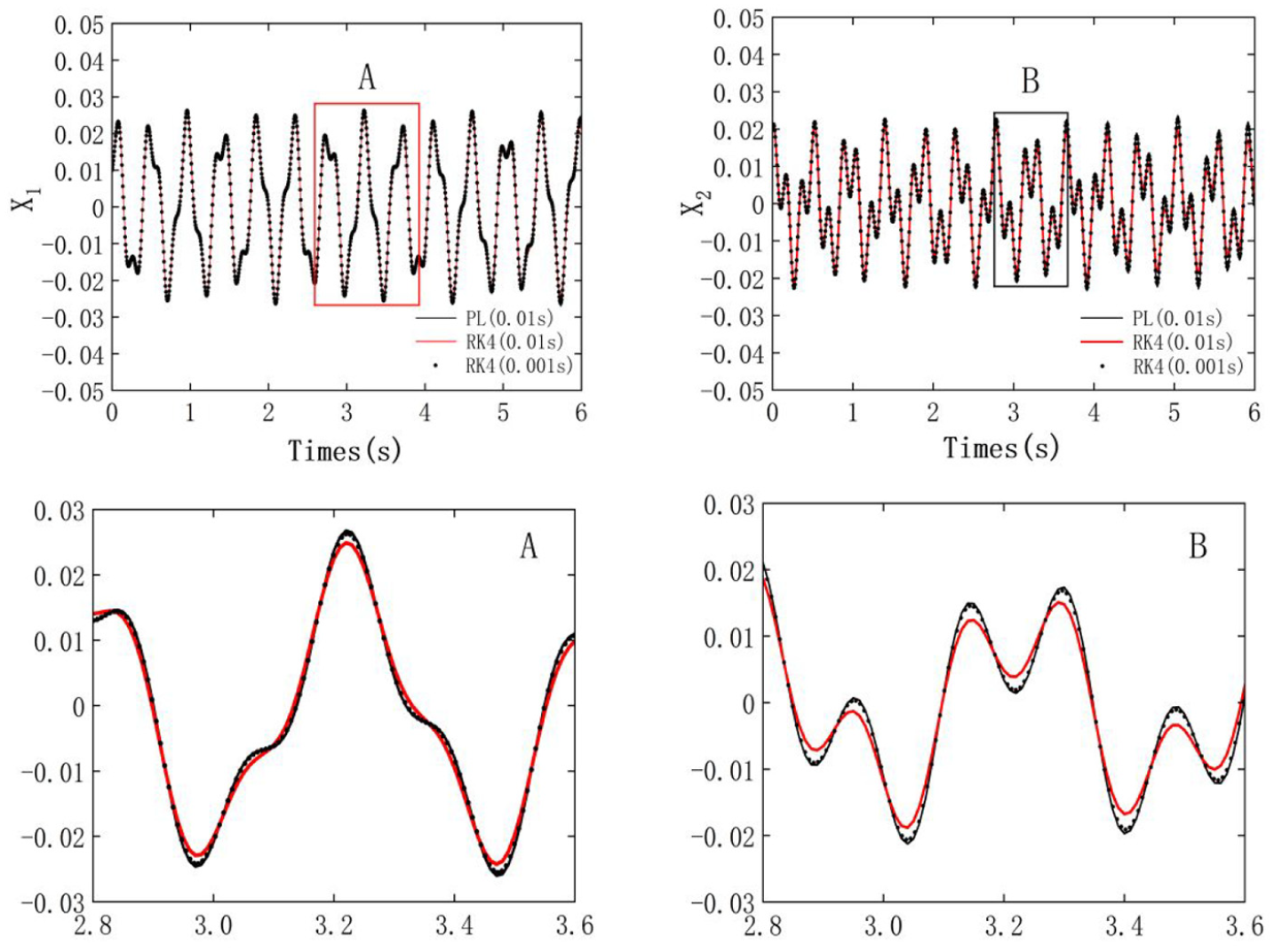
Figure 8 shows the displacement responses of the SDCSF. It follows that the accuracy of PL results is more accurate than RK within same time step; but PL solutions with time step 0.01 s are more approximately approached to RK4 with time step 0.001 s. As shown in Table 6, computational speed of the PL method is faster than RK when calculating SDCSF, and the CPU time required in solving the SDCSF is longer than that of SCS and SDCS in time step 0.01 s because of the presence of damping and external excitation.

Figure 8.

Displacement response of SDCSF $({\omega }_{1,1}=15.811,{\omega }_{1,2}=17.321,{\omega }_{2,2}=20,{\xi }_{1,1}=30,{\xi }_{1,2}=20,{\xi }_{2,2}=10,a=50,\omega =160,x_1(0)=0.01,x{\prime }_1(0)=0.1,x_2(0)=0.02,x{\prime }_2(0)=0.2.)$ .

Table 6.

SDCSF computation time in time history 30 s.

Numerical method	Time step(s)	Iterations	CPU times
RK4	0.001	30000	4.943750
RK4	0.01	3000	0.457751
PL	0.001	30000	3.062512
PL	0.01	3000	0.371920

CPU: central processing unit; RK: Runge-Kutta; PL: Piecewise-Laplace.

Convergence analysis of the PL method

The convergence of the PL method in calculating above three systems is discussed, as illustrated in Figures 9–11.

Figure 9.

Convergence of the solution of SCS by the PL method $({\omega }_{1,1}=22.361,{\omega }_{1,2}=20,{\omega }_{2,2}=17.321,x_1(0)=0.01,x{\prime }_1(0)=0.1,x_2(0)=0.02,x{\prime }_2(0)=0.2.)$ .

Figure 10.

Convergence of the solution of SCDS by the PL method $({\omega }_{1,1}=22.361,{\omega }_{1,2}=20,{\omega }_{2,2}=17.321,{\xi }_{1,1}=10,{\xi }_{1,2}=5,{\xi }_{2,2}=2,x_1(0)=0.01,x{\prime }_1(0)=0.1,x_2(0)=0.02,x{\prime }_2(0)=0.2.)$ .

Figure 11.

Convergence of the solution of SCDSF by the PL method $({\omega }_{1,1}=15.811,{\omega }_{1,2}=17.321,{\omega }_{2,2}=20,{\xi }_{1,1}=30,{\xi }_{1,2}=20,{\xi }_{2,2}=10,a=50,\omega =160,x_1(0)=0.01,2x{\prime }_1(0)=0.1,x_2(0)=0.02,x{\prime }_2(0)=0.2.)$ .

It can be seen that when N = 1000, the numerical results obtained by the PL method are deviated from the accurate value (AV). When N = 2000, the deviation of the numerical solution is reduced. Finally, when N = 20,000, the curve obtained by the PL method is coincident with that of AV. It is indicated that the numerical value obtained by the PL method is approached to the AV as the value of N is gradually increased. Obviously, parameter N is an important factor to control the precision of numerical results and speed of convergence. Therefore, when the value of N is increased, the calculation can converge faster and the precision of the PL method is improved. In order to obtain the high-precision results and faster convergence for solving the coupling dynamics systems, it is better to select a sufficiently large value of N.

Conclusion

In this paper, a new numerical computation method is introduced, and some important conclusion should be stressed as the following.

1. When solving the coupling system by using the traditional RK method, high order differential equations of dynamic system are usually descended into multiple first-order differential equations. In this way, crucial dynamic property of the original system may be neglected or simplified, which leads to the computational error when searching solution for dynamic model encountered in actual engineering. However, solving differential equations above with the PL method, the semi-analytical solution of systems is obtained directly through the derivation of equation. Therefore, the physical properties of systems are well preserved. In addition, the whole-time interval is divided into many tiny intervals by the PL method, and the solution is continuous on each interval. In this case, the accuracy of numerical solution of the PL method is better than the RK method, which is demonstrated by numerical analysis.

2. The computed efficiency of the PL and RK methods are compared through statistics of operation time of CPU during computing process. The CPU time taken by the PL method is less than the RK method in the same time steps, which indicates that the PL method is more efficient than the RK4 method. The main reason is that value continuity of two adjacent truncation points is maintained by using the PL method, which simplifies the solving process and saves the calculated time, while the RK4 method combining iterative and averaged slope to search solutions, which makes the solution process more complicated.

3. The numerical results of the PL method reflect the essence of dynamic system, since the PL method keep the physical characteristics of dynamic system. The precision of the solution obtained by the PL method is related to the value of N. This article is an exploratory study for implementation of the PL method in coupling systems. Therefore, the classic two-degree freedom systems are considered, whether the PL method is suitable to solve problems of multi-degree freedom system should be further verified in our next work.