Sage Journals: Discover world-class research

Abstract

Hydrodynamic effects of mussel farms have attracted increased research attentions in recent years. The understanding of the hydrodynamic impacts is essential for predicting the sustainability of mussel farms. A large mussel farm includes thousands of mussel droppers, and the combined drag on the mussel droppers is sufficient to possibly affect the longevity of the entire long-lines. This article intends to study the drag and wake of an individual long-line mussel dropper using computational fluid dynamics approaches. Two equivalent rough cylinders, namely, Curved-Model and Sharp-Model, have been utilized to simulate the mussel dropper, and each rough cylinder is assigned with surface roughness. The porosity is not considered in this article due to its complexity from inhalant and exhalant of mussels. Two-dimensional laminar simulations are conducted at Reynolds number from 10 to 200, and three-dimensional large eddy simulations are conducted at subcritical Reynolds number ranging from 3900 to $10^{5}$ . The results show that larger drag coefficients and Strouhal numbers are attributed to surface roughness and sharp crowns on the rough cylinder. The obtained drag coefficient ranges from 1.1 to 1.2 with respect to the diameter of the mussel dropper and the peak value of the tidal velocities. Wakes behind rough cylinders fluctuate more actively compared to those of smooth cylinders. This research work provides new insight for further investigations on hydrodynamic interactions between fluid and mussel droppers.

Keywords

Computational fluid dynamics drag and wake long-line mussel tidal current aquaculture farms

Introduction

According to the report from Food and Agriculture Organization (FAO), almost 109 molluscs species have been cultivated in aquaculture farms all over the world.¹ Among all these molluscs, mussel farming is the most popular aquaculture activity with a very rapid growth due to the characteristics of carbon sequestration and environmental friendliness. The suspended long-line culture is the most common way for growing mussel. Long-line structures are approximately 100 to 200 m in length and consist of two parallel backbone ropes. The crop ropes (mussel droppers) are hung vertically from the backbone ropes down to 10 to 15 m of the water column. The commonly used surface mussel long-line is depicted in Figure 1.

Figure 1.

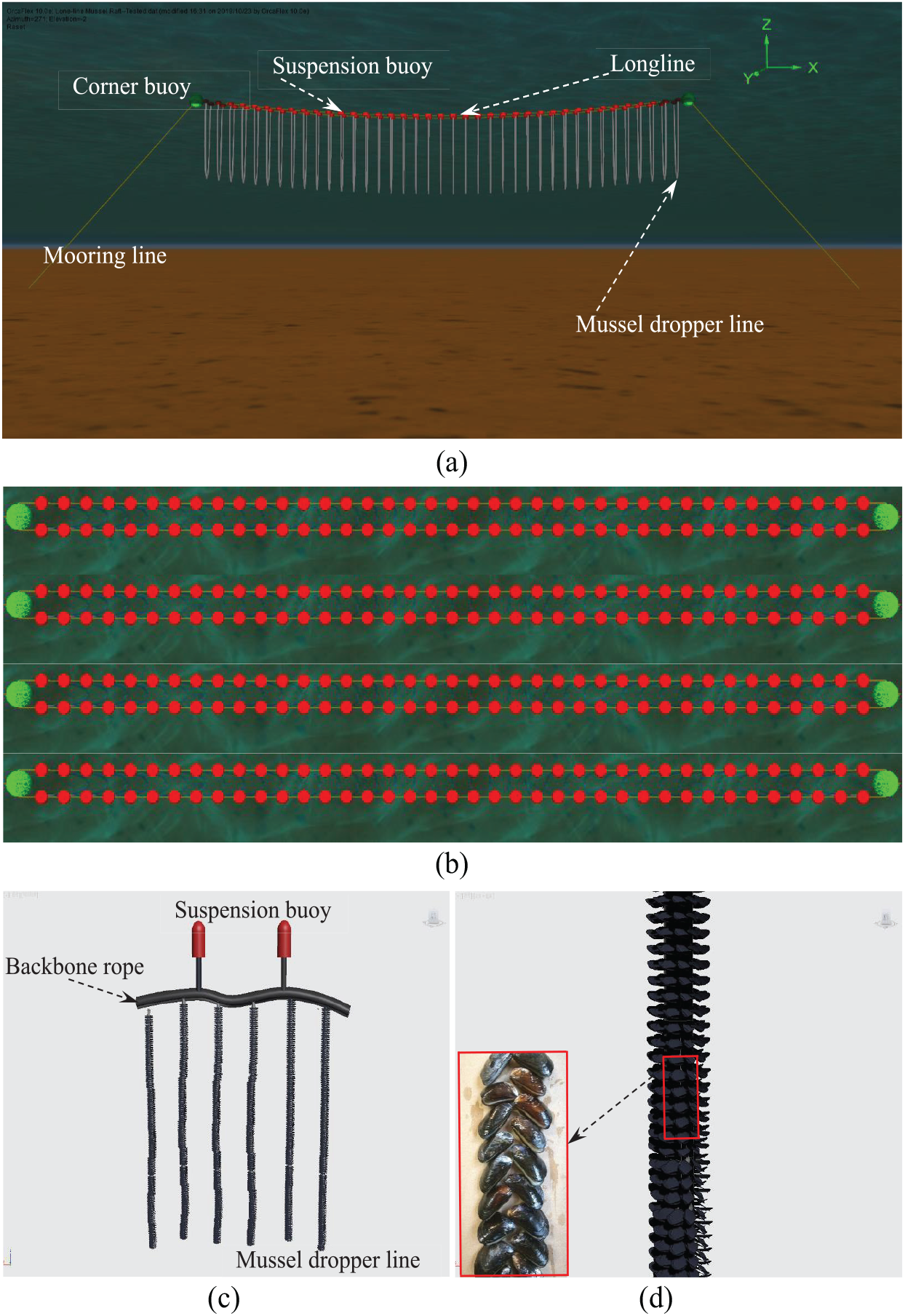
Schematics of the long-line: (a) elevation view, (b) plan view, (c) mussel dropper line arrangement, and (d) close-up view of the mussel dropper.

Large-scale, open-water mussel farming is a sustainable means of providing food to satisfy human demand. However, offshore harsh environment leads to challenges for structure implementation, namely, the movement of the long-lines and the supporting structures induced by the impacts of waves and current, and unpredictable crop losses. The interactions between high energy waves, tidal current, and the long-lines significantly affect the stability of the structures.²

Previous works investigated the suspended mussel droppers as rough cylinders, and the empirical values of hydrodynamic coefficients (these are drag and inertia coefficients), $C_{D} = 1.7$ and $C_{M} = 2.0$ , have been obtained.³ Hydrodynamic coefficients of the mussel droppers can be affected by the Keulegan–Carpenter (KC) number,⁴ and the drag coefficients obtained under steady flow cannot be applied to wave situations.^5,6 Previous studies showed that the current velocity decreased as the flow passed the mussel farm.⁷ This velocity reduction has been well documented.^4,8 The dynamic response of the submersible mussel raft in waves and current has been investigated using the software package Aqua-FE,^9,10 which is developed by the University of New Hampshire.^11,12 More recently, a computational fluid dynamics (CFD)–based approach has been utilized to study the hydrodynamic behavior of the mussel farm in current.¹³

Most of the previous research works concentrated on the dynamic response and shielding effects of the mussel farm. The understanding of hydrodynamic coefficients of the mussel dropper still has not been completely settled down. Also, the effects of mussel shell on the flow pattern of the mussel dropper are barely documented. With these two concerns, this study intends to examine the impact of surface roughness of the mussel dropper on the drag and wake of an individual dropper. Two different equivalent cylinders with the same roughness of the mussel dropper have been tested under two CFD schemes.

It is noted that the inhalant and exhalant siphons allow mussels to exchange flow to acquire nutrients from the surroundings, causing the mussel dropper more likely to be porous instead of solid. Previous investigations showed that a porous cylinder had a drag coefficient 20% smaller than the solid cylinder, and the vortex shedding was also weaker behind the porous cylinder.¹⁴ Therefore, to study the drag and wake of the mussel dropper, both roughness and porosity should be considered. However, we focus mostly on the effects of roughness on the drag and wake of the mussel dropper in this article, and thus, the assessment was conducted without considering the complexity of the porosity.

The remainder of the article is organized as follows. In the “Methodology” section, we first introduce the mathematical formulations and numerical discretization of the CFD approaches, which include a two-dimensional (2D) laminar simulation and a three-dimensional (3D) large eddy simulation (LES). The results of the simulations are presented in section “Results and discussion.” The conclusions are given in section “Conclusion.”

Methodology

Laminar simulation

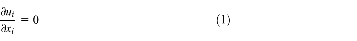
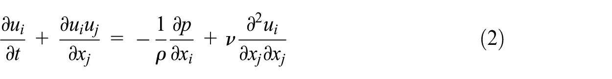
Two-dimensional simulations are conducted for laminar flow around smooth and rough cylinders at Reynolds numbers $(Re)$ from 10 to 200 in OpenFOAM. Previous research reported that the wake behind the smooth cylinder remains 2D when Reynolds number $(Re)$ is smaller than 200, otherwise the wake is 3D.¹⁵ In this case, any 2D simulation is infeasible to represent the physical traits of the flow if the Reynolds number $(Re)$ is greater than 200.

We assume the flow is incompressible. The governing Navier–Stokes equations for an incompressible 2D flow regarding the conservation of mass, momentum, and energy are defined as

\begin{matrix} \frac{\partial u_{i}}{\partial x_{i}} = 0 \end{matrix}

(1)

\begin{matrix} \frac{\partial u_{i}}{\partial t} + \frac{\partial u_{i} u_{j}}{\partial x_{j}} = - \frac{1}{ρ} \frac{\partial p}{\partial x_{i}} + ν \frac{\partial^{2} u_{i}}{\partial x_{j} \partial x_{j}} \end{matrix}

(2)

where $u_{i}$ are the velocity components in the Cartesian coordinates $x_{i}$ ; $x_{1}$ and $x_{2}$ represent the components in $x$ and $y$ directions, respectively; $p$ is the pressure; $ρ$ is the fluid density; and $ν$ is the kinematic viscosity of the fluid. The non-dimensional parameters relevant to the present flow problems are given as follows

Reynolds number, Re = \frac{U_{\infty} D}{ν}

Strouhal number, St = \frac{fD}{U_{\infty}}

Surface roughness = \frac{K_{s}}{D}

Drag coefficient, C_{D} = \frac{2 F_{D}}{ρ D L_{cyl} U_{\infty}^{2}}

Lift coefficient, C_{L} = \frac{2 F_{L}}{ρ D L_{cyl} U_{\infty}^{2}}

where $U_{\infty}$ is the free stream velocity, $f$ is the vortex shedding frequency, and $D$ and $L_{cyl}$ are the diameter and length of the cylinder, respectively.

The governing equations in this study are a set of partial differential equations (PDEs). We utilize the finite volume method (FVM) with structured grids to discretize these PDEs. The computational domain is represented by numerical grids at which the variables can be transferred and calculated. Structured grids include three basic topologies: H-, O-, and C-grids. All three topologies have been employed for investigating smooth cylinder. The names of the grid topology are derived from the shapes of the grid lines.¹⁶

The discretization is to convert the PDEs into non-linear algebraic equations. For unsteady flows, an elliptic problem has to be solved at each time step. Steady flows are solved by an equivalent iteration scheme, and then problems turn out to be solutions of linear equation systems. Some convergence criteria need to be checked after all iterations are finished. The repeat of the loop depends on the condition if the convergence is satisfied. We utilized commercial code ANSYS ICEM to create three different computational domains for smooth circular cylinder as depicted in Figure 2.

Figure 2.

Two-dimensional computational domains of flow around smooth circular cylinder and boundary conditions: H-, O-, and C-grids.

Different grid topologies used in this study enable validation for grid independence study under the same algorithm scheme. The most optimal grid topology can be identified after comparison, to meet the accuracy requirement and the computational efficiency. For these three different grids, the boundary conditions are set as follows:

H-grid: we set left side as flow inlet $(Γ_{in})$ and right side as pressure outlet $(Γ_{out})$ ; slip walls are implemented on top $(Γ_{top})$ and bottom $(Γ_{bottom})$ to model an undisturbed flow channel; and the cylinder wall is set as no-slip wall to ensure there is no relative movement between the boundary and the fluid layer.

O-grid: left and right sides are set as flow inlet $(Γ_{in})$ and pressure outlet $(Γ_{out})$ , respectively. No-slip wall is implemented on the cylinder wall.

C-grid: left, top, and bottom sides are set as flow inlet $(Γ_{in})$ , which provides slip walls on top and bottom sides as boundary conditions; the velocities on top and bottom sides are free stream velocities. The right side of the domain is set as pressure outlet $(Γ_{out})$ . No-slip wall is implemented on the cylinder wall.

Only if stated, otherwise, all positions and length scales are normalized by the characteristic length $(D)$ . The Reynolds number $(Re)$ of the flow is determined by the characteristic length $(D)$ , the kinematic viscosity of the fluid $(ν)$ , and the free stream velocity $(U_{\infty})$ . On the surface of the cylinder, a constant value of temperature is prescribed.

The coupled scheme is implemented for pressure–velocity coupling where convective term discretization is conducted by semi-implicit method for pressure-linked equations (SIMPLE) schemes.¹⁷ The spatial discretization of the pressure and momentum is conducted through second-order and second-order upwind differencing schemes, respectively. The temporal discretization is conducted using second-order implicit differencing scheme. The algebraic equations are solved by the Gauss–Seidel iterative method in conjunction with the Algebraic Multigrid (AMG) solver. The AMG method greatly reduces the number of required iterations (and thus, CPU time) to obtain a converged solution, particularly when the model contains large number of control volumes. The time step varies from 0.01 to 0.05 for steady and unsteady flow conditions, respectively. The convergence criteria for the inner iterations (time steps) are set as 10⁻⁹ for the discretized continuity, momentum, and energy equations.

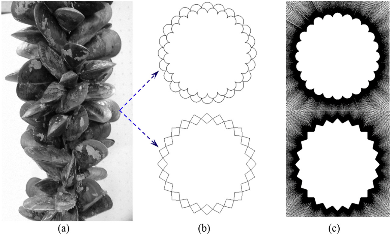
Mussels form dense aggregations which grow on suspended aquaculture long-lines. The diameter of the mussel droppers varies as mussels mature. For example, the typical averaged diameter of the mussel dropper approaches approximately 0.15–0.2 m, with the typical peak tidal velocities of the mussel farm ranging from 0.05 to 0.2 m/s, Reynolds numbers of a mussel dropper are between $10^{3}$ and $10^{5}$ . With these Reynolds numbers, 2D simulations seem infeasible to predict the hydrodynamic effects of the long-line mussel droppers. However, the general flow characteristics can be obtained from 2D simulations for comparison. Besides, it is difficult to create the grids of the mussel dropper due to its geometrical sophistications; therefore, we utilize equivalent rough cylinders to represent mussel droppers in this article. The 2D equivalent rough cylinders are depicted in Figure 3.

Figure 3.

Two-dimensional equivalent rough cylinder models: (a) real mussel dropper, (b) geometries of equivalent rough cylinders, and (c) grids of equivalent rough cylinders (picture of real mussel dropper is reproduced from Plew²).

Based on the geometries of the equivalent rough cylinders, we define them as Curved-Model and Sharp-Model. By adding the crowns in the geometries of the rough cylinders, mussel shells can be represented without losing the geometrical characteristics. Surface roughness, $K_{s} / D = 0.048$ and $0.094$ , has been assigned for each rough cylinder. We have to create the geometries and grids of the rough cylinders in a symmetric way; otherwise, the failure cannot be avoided with any of the unsymmetrical geometries. The boundary conditions, the spatial and temporal discretization, remain same with the conditions for smooth cylinders.

LES

Three-dimensional LES are conducted at Reynolds number $Re = 3900$ to $10^{5}$ . Three-dimensional incompressible Navier–Stokes equations are discretized by structured hexahedral grids in a FVM scheme in OpenFOAM. The filtered continuity equation and the momentum and energy equation are given as

\begin{matrix} \frac{\partial \bar{u_{i}}}{\partial x_{i}} = 0 \end{matrix}

(3)

\begin{matrix} \frac{\partial \bar{u_{i}}}{\partial t} + \frac{\partial \bar{u_{i}} \bar{u_{j}}}{\partial x_{j}} = - \frac{1}{ρ} \frac{\partial \bar{p}}{\partial x_{i}} + ν \frac{\partial^{2} \bar{u_{i}}}{\partial x_{j} \partial x_{j}} - \frac{\partial τ_{ij}}{\partial x_{i}} \end{matrix}

(4)

where $\bar{u_{i}}$ are the filtered velocity components in the Cartesian coordinates $x_{i}$ ; $x_{1}$ , $x_{2}$ , and $x_{3}$ represent the components in $x$ , $y$ , and $z$ directions, respectively; $\bar{p}$ is the filtered pressure; and $τ_{ij} = \bar{u_{i} u_{j}} - \bar{u_{i}} \bar{u_{j}}$ are the sub-grid scaled stresses. The Smagorinsky–Lilly model is employed in this study. The turbulent eddy viscosity is given as $ν_{t} = (C_{s} Δ)^{2} \sqrt{2 \bar{S_{ij}} \bar{S_{ij}}}$ , where $C_{s} = 0.1$ , $Δ$ is the volume of the cell, and $\bar{S_{i j}} = \frac{1}{2} (\frac{\partial \bar{u_{i}}}{\partial x_{j}} + \frac{\partial \bar{u_{j}}}{\partial x_{i}})$ is the rate-of-strain tensor.

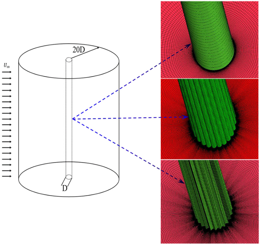
To ensure the grid orthogonality,¹⁸ the computational domain for 3D simulations utilizes an O-grid, which is extruded by a 2D O-grid in ANSYS ICEM. The diameter of the 3D O-grid is 40D, where $D$ is the diameter of the cylinder. With this domain size, both the accuracy requirement and the computational efficiency are satisfied. The domains for smooth and rough cylinders remain same for the sake of comparison, as depicted in Figure 4.

Figure 4.

Three-dimensional computational domains of flow around smooth and rough cylinders.

We describe the grids of the 3D computational domain by polar coordinates. Cell numbers are presented by $N_{r}$ , $N_{θ}$ , and $N_{z}$ , where $N_{r}$ is the cell number in the direction of diameter, $N_{θ}$ is the cell number in the direction of circumference, and $N_{z}$ is the cell number in the direction of span-wise. Particularly, we conduct the grid independence study at $Re = 3900$ and compare the results with those of previous work.

The first layer of the cell is set as $3.2 \times 10^{- 4} D$ to ensure $y^{+} \leq 1$ in LES of turbulent flow. The grids are refined as Reynolds number increases, for $Re = 10^{5}$ , and the first layer of the cell is set as $1.4 \times 10^{- 5} D$ . The Kolmogorov length scale $l_{ν} = (ν^{3} / ε)^{1 / 4}$ , where $ν$ is the kinematic viscosity of the fluid and $ε = u_{rms}^{3} / L_{w}$ is the energy dissipation rate, in which $L_{w}$ is the characteristic length scale in the wake behind the cylinder.¹⁹ The present grid scale could at least capture 20 times the Kolmogorov length scale, which satisfies the sub-grid modeling in the present LES cases. The boundary conditions for present LES simulations are set as follows:

Inflow boundary: the left portion of the cylindrical domain is set as velocity inlet, where the flow is uniformly distributed with the turbulence intensity of 1%.

Outflow boundary: the pressure outlet is imposed at the right portion of the cylindrical domain. A Neumann boundary condition $(\partial u / \partial x = \partial v / \partial y = \partial w / \partial z = 0)$ is used for the velocities.

Surface boundary: for the surface of the cylinder, the Dirichlet boundary condition is used for the velocities $(u = v = w = 0)$ . The zero-gradient condition is used for the pressure.

Span-wise boundary: the periodic condition is implemented for the span-wise direction of the cylinder.

The pressure implicit splitting of operators (PISO) scheme is utilized for the velocity–pressure coupling. Pressure and momentum are discretized by second-order and bounded central differencing schemes, respectively. For the temporal discretization, the bounded second-order implicit differencing scheme is used. Time step is set as $Δ t = 2 \times 10^{- 4}$ to ensure Courant–Friedrichs–Lewy (CFL) number is smaller than 1.

Numerical accuracy

To evaluate the grid sensitivity and numerical accuracy, different computational domains and cell numbers have been examined for 2D laminar and 3D LESs, respectively. The descriptions of different computational domains (H-, O-, and C-grids) for smooth cylinders are illustrated in Table 1. The comparison of different grids is for one thing to conduct the validation, and for another, to select the most optimal grid topology for further rough cylinder simulations.

Table 1.

Different computational domains for 2D laminar flow around smooth cylinder.

Domain	H-grid	O-grid	C-grid
Small	25D× 20D	R =10D	R =10D, L=15D
Medium	30D× 20D	R =15D	R =15D, L=15D
Large	50D× 20D	R =25D	R =25D, L=25D

$D$ is diameter of the cylinder, $R$ is the radius of O- and C-grids, and L is the length of the connected part in the C-grid.

Previous numerical simulation¹⁵ found that the obtained Strouhal number $(St)$ was slightly overestimated if the width of the H-grid domain was less than 10D. Thus, the width of the H-grid domain should at least be larger than 10D. It has been suggested that H-grid domain with a 30D × 20D dimension could minimize the computing time without losing accuracy.²⁰ The numerical study of laminar flow passing a smooth cylinder with O-grid showed that a diameter of the domain with 40D predicted accurate results.²¹ Based on these previous researches, we create domains accordingly and compare different grid topologies in this article. The comparisons of drag coefficients $(C_{D})$ and Strouhal number $(St)$ for smooth cylinders in different 2D grids are shown in Figures 5 and 6, respectively.

Figure 5.

Comparisons of drag coefficient $(C_{D})$ for smooth cylinders in different 2D grids.

Figure 6.

Comparisons of Strouhal number $(St)$ for smooth cylinders in different 2D grids.

Figure 5 shows that the overall dependences of drag coefficients on Reynolds number are as expected, and the effect of domain dimension on drag coefficient is insignificant. Since all the 2D simulations are conducted in the same algorithm scheme, if a great discrepancy occurs, there must be some unexpected errors need to be checked from the beginning of the loop. For the H-grid under steady flow conditions $(Re \leq 50)$ , the domain dimension almost has no effect on the drag coefficients. For the H-grid under unsteady flow conditions $(50 \leq Re \leq 200)$ , the large domain acquired smaller drag coefficients compared to those from other domains. For the O-grid under steady flow conditions, small domain obtained higher drag coefficients; for the O-grid under unsteady flow conditions, the drag coefficient is higher at the large domain. For the C-grid, drag coefficients are relatively high in the large and the small domains.

There are obvious differences in the dependence of Strouhal number on Reynolds number (Figure 6). Small domain obtained large Strouhal number, which verified the previous numerical investigation.¹⁵ The Strouhal numbers obtained from the medium and the large domains are very close to each other. We then select the medium domain with respect to the requirement of computational efficiency and numerical accuracy. With this medium domain, the drag coefficient and Strouhal number obtained in different grids are compared (Figure 7).

Figure 7.

Comparisons of drag coefficient $(C_{D})$ and Strouhal number $(St)$ for smooth cylinders in three different 2D grids (H-, O-, and C-grids).

Figure 7 shows that for the steady flow conditions, the drag coefficients obtained from H-grid are larger than that from others, while the drag coefficients obtained from C-grid are smaller than that from others. For the unsteady flow conditions, the results are almost same for these three different grids. The same trend of Strouhal number can be achieved from different grids under medium domain dimensions. The vorticities behind smooth cylinders in different grids are demonstrated in Figure 8.

Figure 8.

Comparisons of vorticities behind smooth cylinders in different 2D grids.

The vorticities generated in C-grid appear quite sparse in far field. H- and O-grids predict similar vortex patterns. The comparisons of drag coefficients and Strouhal numbers show that the medium domain is compatible to meet the requirement of computational efficiency and numerical accuracy. Therefore, we utilize O-grid to conduct the simulations for rough cylinder without any further verification, and the domain dimension is set as 30D based on smooth cylinder cases. The cell numbers and 3D LES grid independence studies for smooth and rough cylinders at Reynolds number $Re = 3900$ are illustrated in Table 2.

Table 2.

Numerical accuracy studies of different cell numbers $(Re = 3900)$ .

Cylinder	$N_{r}$	$N_{θ}$	$N_{z}$	$C_{D}$	$S_{t}$
Smooth-1	200	200	150	0.976	0.21
Smooth-2	200	200	200	0.981	0.21
Smooth-3	200	200	250	0.979	0.21
Cheng et al.¹⁸	256	256	64	0.980	0.21
Rough-curved model	200	200	200	0.997	0.25
Rough-sharp model	200	200	200	1.091	0.26

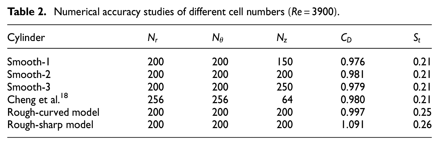
The effect of the cell numbers on drag coefficient and Strouhal number is insignificant for the smooth cylinders. The present simulation results for smooth cylinder are in good agreement with previous work conducted by LES.¹⁸ Therefore, $N_{r} = 200$ , $N_{θ} = 200$ , and $N_{z} = 200$ have been selected for the simulations of the rough cylinders with the total cell numbers of around 8 million. Given the surface roughness $K_{s} / D = 0.048$ for curved and sharp models of the rough cylinder, the 3D LES results can be obtained. As shown in Table 2, the drag coefficient and the Strouhal number increase from Curved-Model to Sharp-Model, which demonstrates that sharp crowns on the equivalent rough cylinder have more effects on wake fluctuations.

Results and discussion

Drag coefficient and Strouhal number

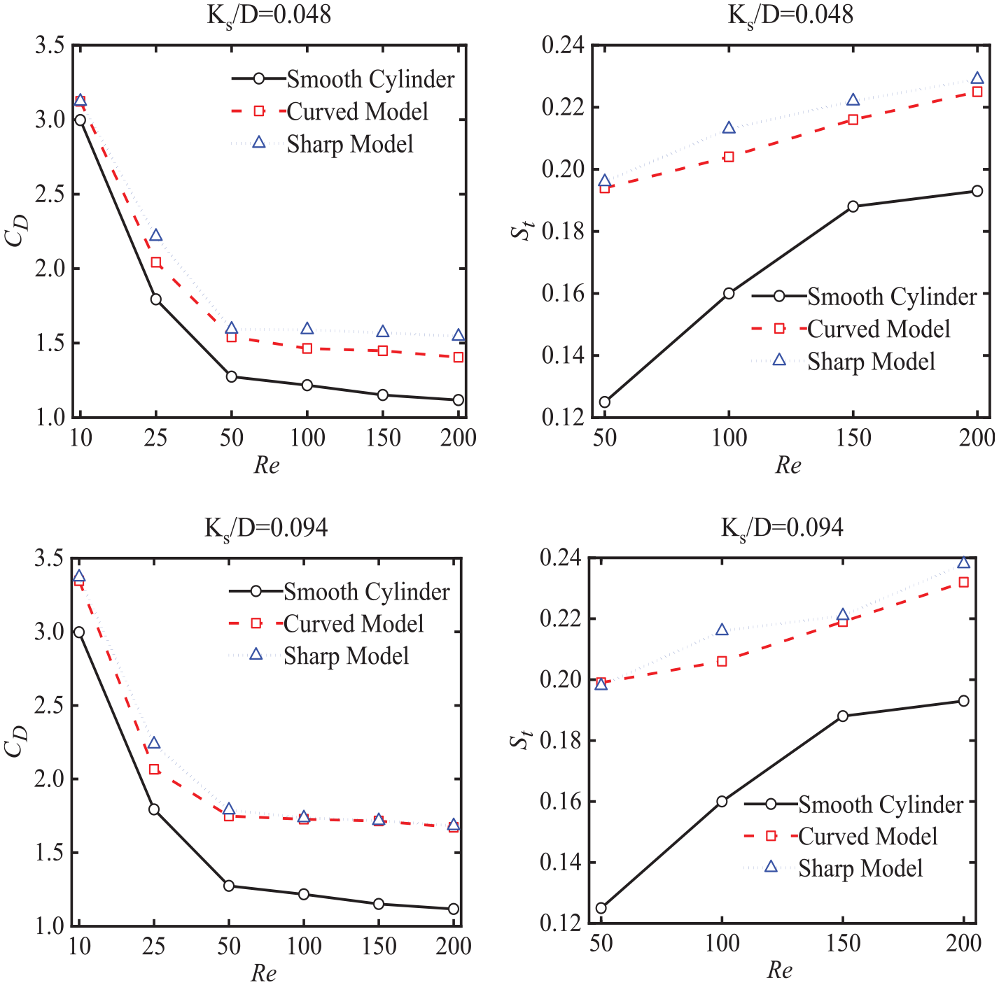
Two equivalent rough cylinders (Curved-Model and Sharp-Model) are utilized to model the mussel droppers. Each equivalent rough cylinder has been assigned surface roughness $K_{s} / D = 0.048$ and $0.094$ in 2D laminar simulations. The effects of surface roughness on drag coefficient and Strouhal number are exhibited in Figure 9. The crowns on the rough cylinders with different shapes have been utilized to represent the mussel shells. Figure 10 demonstrates the effects of different crown shapes on drag coefficient and Strouhal number.

Figure 9.

Effects of surface roughness on drag coefficient and Strouhal number.

Figure 10.

Effects of crown shapes on drag coefficient and Strouhal number.

Similar with the trend of smooth cylinder, drag coefficients of the equivalent rough cylinders decrease with the increase in Reynolds numbers, while Strouhal number increases with the increase in Reynolds numbers. In terms of effect of surface roughness, drag coefficient and Strouhal number increase with the surface roughness. In particular, Strouhal number ranges from 0.2 to 0.24 for rough cylinder in laminar flow. The considered range for smooth cylinder is from 0.1 to 0.2 when Reynolds number is below 200, demonstrating that the surface roughness has significant effect on vertex shedding of the rough cylinders.

Figure 10 shows that sharp crown has more effects on drag coefficient and Strouhal number. Drag coefficients and Strouhal numbers of Sharp-Model are greater than that of Curved-Model. As the surface roughness increases, there are oscillations in the Strouhal number, which indicates that sharp crowns induced more violent flow oscillations.

Differing from the 2D simulations, the flow oscillations become even more violent at subcritical Reynolds number in 3D LESs. To study the vertex shedding of the rough cylinders, Figure 11 exhibits the dependence of lift coefficient on non-dimensional time at $Re = 3900$ for Curved-Model.

Figure 11.

Dependence of drag and lift coefficients on non-dimensional time at $Re = 3900$ for Curved-Model.

Figure 11 shows that the oscillation of lift coefficient is periodic because of the periodic boundary condition on the span-wise direction. Particularly, this periodic oscillation shows more regular pattern after 20 s. However, the wake oscillations of the Sharp-Model exhibit more chaotically at $Re = 3900$ , as shown in Figure 12.

Figure 12.

Dependence of lift coefficients on non-dimensional time at $Re = 3900$ for Sharp-Model.

The oscillation of lift coefficient is partially induced by periodic boundary conditions. Besides, due to the blocking effects of the sharp crowns around the rough cylinder, more active oscillation occurs compared with the situations for Curved-Model. Lift coefficient at the initial stage has larger amplitude around 0.05, as the wake development, boundary layer shear flow transports from 2D to 3D, the averaged amplitude of lift coefficient reduces approximately 30% compared with that of the primary stage.

To evaluate the effect of Reynolds number on drag coefficient at all considered subcritical Reynolds number, Figure 13 presents the dependence of drag coefficients on Reynolds numbers for smooth and equivalent rough cylinders. Given the surface roughness $K_{s} / D = 0.048$ , the drag coefficients of the mussel dropper can be obtained.

Figure 13.

Dependence of drag coefficients on Reynolds numbers for smooth and equivalent rough cylinders $(K_{s} / D = 0.048)$ .

The overall trends of the drag coefficients for smooth and rough cylinders in this study are similar to Hoerner’s report.²² The drag coefficient of the rough cylinder ranges from 1.1 to 1.2 at subcritical Reynolds numbers. Even with the same surface roughness, the drag coefficients show different values due to the crown shapes on the surface of the rough cylinders. The drag coefficients for the Sharp-Model are larger than that of others. When Reynolds number is less than O( $10^{5}$ ), drag coefficients tend to increase, but when Reynolds number is larger than O( $10^{5}$ ), the drag coefficients increase slowly and approach a platform. The mussel dropper is represented by equivalent rough cylinder as an approximate approach in this study. We conclude that the drag coefficient of the mussel dropper ranges from 1.1 to 1.2 at subcritical Reynolds numbers.

Wake and flow pattern

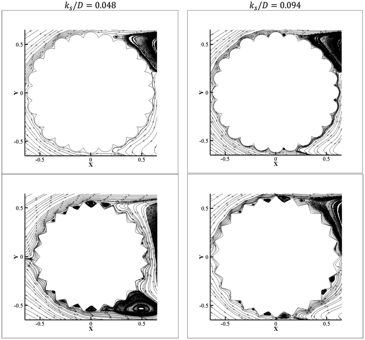
To observe the effects of surface roughness on the flow pattern, Figure 14 presents the 2D streamlines of Curved-Model and Sharp-Model at $Re = 150$ . For the Curved-Model, the streamlines vary as the surface roughness increases, and there are a few small eddies behind the curved crowns. Quite obviously for the Sharp-Model, there are even more small eddies behind the sharp crowns. The existence of these small eddies results in energy attenuations which enlarges drag coefficients. Moreover, more active oscillations induced from sharp crowns are responsible for higher Strouhal number. The comparison of streamlines demonstrates that Sharp-Model represents mussel dropper more precisely with the small eddies behind the sharp crowns.

Figure 14.

Streamlines of flow around different equivalent rough cylinders at $Re = 150$ .

When Reynolds number approaches 3900, the wake behind the rough cylinder is completely turbulent flow, but the boundary layer is still not fully developed as turbulent flow. The separation of the flow occurs when flow passes the rough cylinder, and then the flow rolls back to the wake to be absorbed onto the cylinder again, as shown in Figure 15(a).

Figure 15.

Flow around Curved-Model at $Re = 3900$ : (a) onset of turbulent vorticity and (b) turbulent kinetic energy (vorticity: $- 10 \leq ω \leq 10$ ).

Turbulent kinetic energy (TKE) varies at different wake positions, in particular, TKE approaches its peak in the wake roll-back position (position B) as shown in Figure 15(b). Position A in Figure 15(a) indicates that the wake is rolling back to form a secondary wake. TKE is defined in the following equation

\begin{matrix} k = \frac{1}{2} (\bar{{(u')}^{2}} + \bar{{(v')}^{2}} + \bar{{(w')}^{2}}) \end{matrix}

(5)

where $u'$ , $v'$ , and $w'$ are the turbulent fluctuation velocities in x, y, and z directions, respectively. As the rough cylinder switches from Curved-Model to Sharp-Model, the turbulent wake forms 3D flow pattern as shown in Figure 16.

Figure 16.

Turbulent vorticity of Sharp-Model at $Re = 3900$ (vorticity: $- 10 \leq ω \leq 10$ ).

To study the effects of crowns around the rough cylinder on the wake in the near field, Figure 17 exhibits the turbulent oscillation velocities along the centerline of the cylinder. The comparison between smooth and rough cylinders is conducted for further analysis. In Figure 17, $u$ is the turbulent fluctuation velocity along the centerline of the cylinder and U is the free stream velocity.

Figure 17.

Time-averaged stream-wise velocity along the wake centerline at $Re = 3900$ . (The stream-wise velocities of Curved-Model, Sharp-Model, and Cheng et al. are compared in the right figure using the same symbols in the left figure.)

The overall trend of the velocity distribution is similar to the demonstration in Cheng et al.¹⁸ The turbulent fluctuation velocity decreases along the wake centerline in the near-wake region to reach a minimum value and then increases in the far-wake region. The velocities for the Curved-Model and Sharp-Model are smaller compared to the case of smooth cylinder, due to the blockage of the crowns on the equivalent rough cylinders. Cell numbers utilized in Cheng et al.¹⁸ are about 210 million with $N_{r} = 8192$ , $N_{θ} = 1024$ , and $N_{z} = 256$ . It is much easier to capture the Kolmogorov length scale of the turbulent eddies in the subcritical Reynolds numbers with such refined grids; however, we have to compromise on the computational efficiency as well.

The cell numbers could be the reason that makes the present simulation results slightly different with the results from Cheng et al.¹⁸ For example, the valley value obtained from the present LES is smaller than previous simulation at $y / D = 0$ . In the overall range of $- 0.5 \leq y / D \leq 0.5$ , the velocity shows a U-shaped distribution. The valley value becomes smaller as the crown changes from curve to sharp. This indicates the effects of the crowns on velocity distribution and wake are significant. Thus, it is imperative to choose the appropriate crowns to represent the mussel shells. The velocity distribution decreases to a valley value as $x / D$ increases and then increases in the far field region. Compared with the smooth cylinder, the crown-bounded rough cylinder induced energy dissipation that disturbs the wake, as shown in Figure 18.

Figure 18.

Turbulence kinetic energy (TKE) along the wake centerline at $Re = 3900$ .

Figure 18 demonstrates that the overall trends for smooth and rough cylinders are similar. The velocity is zero in the wake roll-back region from 0.1D to 0.4D. TKE increases as $x / D$ increases and approaches a peak value; it then drops in the far-wake region. Sharp-Model has larger TKE compared with others, because the sharp crowns on the Sharp-Model take more time for the flow to recover in the near-wake region. The blockage caused by sharp crowns enhances energy dissipation.

Q-criterion²³ is utilized to present the iso-surfaces of vorticities in this study. The basic principle is to decompose the velocity gradient $\nabla \cdot U = S + Ω$ , where $S = \frac{1}{2} [\nabla \cdot U + (\nabla \cdot U)^{T}]$ is the rate-of-strain tensor, $Ω = \frac{1}{2} [\nabla \cdot U - (\nabla \cdot U)^{T}]$ is the vorticity tensor, and then Q is defined as $Q = \frac{1}{2} (| Ω |^{2} - | S |^{2})$ . Given $Q = 100 s^{- 2}$ , iso-surfaces of Q-criterion vorticities at $Re = 3900$ and $10^{5}$ are exhibited in Figures 19 and 20, respectively.

Figure 19.

Iso-surface of Q-criterion vorticities at $Re = 3900$ from smooth cylinder to rough cylinder: (a) smooth cylinder, (b) Curved-Model, and (c) Sharp-Model.

Figure 20.

Iso-surface of Q-criterion vorticities at $Re = 10^{5}$ from smooth cylinder to rough cylinder: (a) smooth cylinder (reproduced from Zhang et al.²⁴), (b) Curved-Model, and (c) Sharp-Model.

Figure 19 shows the 3D vorticities behind the cylinders. When the cylinder varies from the smooth to the rough, the vorticity formulations change differently. The vorticity tubes behind the Sharp-Model indicate that the surface roughness, especially the crown shapes, significantly alters the vorticity formulations.

When Reynolds number approaches O( $10^{5}$ ), with the disturbance of sharp crown, the vorticities in the wake of the Sharp-Model form bundles of vorticity tubes, which move with the flow to far field (Figure 20). Vorticity tubes oscillated along the alternative sides of the cylinders interact with each other. During this process, interactions of vorticity tubes and energy loss separate the vorticity tubes into smaller vorticity filaments until final breaking occurs. The whole process keeps repeating with the vortex shedding.

Conclusion

In this article, CFD approaches have been utilized to investigate the drag and wake of a long-line mussel dropper. 2D laminar and 3D LESs were conducted at considered Reynolds numbers. The grid independence study and numerical accuracy were examined for convergence analysis. Two equivalent rough cylinders were used to model the mussel dropper, through which the effect of surface roughness on the drag and wake can be assessed. The conclusions are as follows:

For the smooth cylinder in 2D simulations, the comparisons between three different grids showed that O-grid with domain diameter of 30D could feasibly predict the drag and wake without losing accuracy. For the equivalent rough cylinders in 2D simulations, the drag coefficients increased with the surface roughness. The crowns around the rough cylinder significantly affected the drag coefficient. Sharp crowns resulted in larger drag coefficients than that of others. The streamlines for equivalent rough cylinders were very different from those of smooth cylinders.

The drag coefficient of the rough cylinder ranges from 1.1 to 1.2 at subcritical Reynolds numbers. Sharp crowns induced more energy loss and the wake is more fluctuated. As a result, the Strouhal number was in a range from 0.25 to 0.26. This number was much larger than that of smooth cylinders (around 0.21). The equivalent rough cylinder is an efficient way by which the drag and wake of a mussel dropper can be examined using CFD scheme. The porous characteristics induced by inhalant and exhalant of mussels should be emerged in further studies.

Footnotes

Declaration of conflicting interests

The author(s) declared no potential conflicts of interest with respect to the research, authorship, and/or publication of this article.

Funding

The author(s) disclosed receipt of the following financial support for the research, authorship, and/or publication of this article: This work was financially supported by the National Natural Science Foundation of China (Grant Nos 51679046 and 51909040).

ORCID iD

Hongde Qin

Author biographies

Zhijing Xu earned his PhD in Shipbuilding and Ocean Engineering from the Harbin Engineering University. His research focuses on fluid-structure interactions of cage based and long-line aquaculture, with regards to numerical implementations and physical model tests. He joined the Department of Mechanical Engineering since 2016 at the University of New Hampshire, as a visiting scholar.

Hongde Qin is the director of the National Key Laboratory of Science and Technology on Autonomous Underwater Vehicle, Harbin Engineering University. He obtained a PhD in Shipbuilding and Ocean Engineering from the Harbin Engineering University. His research interests include tracking control of autonomous underwater vehicle systems and hydrodynamics of aquaculture structures.

Peng Li is an associate professor of the College of Shipbuilding Engineering at the Harbin Engineering University. He obtained his PhD in Ocean Engineering from Norwegian University of Science and Technology. His research focuses on hydrodynamic response of open offshore aquaculture structures, with both analytical and experimental approaches.

Rujun Liu has a background in Power Engineering of aircraft, with a MSc in Aerodynamics from the University of New Hampshire. His research focuses on the flow around bluff bodies with wind tunnel experiments and numerical simulations. He is currently working on the vibration of airfoil and vortex dynamics.

References

FAO. The state of world fisheries and aquaculture 2018: meeting the sustainable development goals. Rome: Food and Agriculture Organization of the United Nations, 2018.

Plew

DR.

The hydrodynamic effects of long-line mussel farms. Doctoral Dissertation, Department of Civil Engineering, University of Canterbury, Christchurch, New Zealand, 2005.

Wolfram

Naghipour

On the estimation of Morison force coefficients and their predictive accuracy for very rough circular cylinders. Appl Ocean Res 1999; 21: 311–328.

Stevens

Plew

Hartstein

, et al. The physics of open-water shellfish aquaculture. Aquacult Eng 2008; 38: 145–160.

Sarpkaya

Force on a circular cylinder in viscous oscillatory flow at low Keulegan–Carpenter numbers. J Fluid Mech 1986; 165: 61–71.

Zdravkovich

MM.

Flow around circular cylinders, volume 2: applications. Oxford: Oxford University Press, 1997.

Waite

RP.

The nutritional biology of Pena canaliculus with special reference to intensive mariculture systems. Christchurch, New Zealand: University of Canterbury, 1989, p. 136.

Paul

Grosenbaugh

Submerged coastal offshore mussel aquaculture system (SCOMAS): a multidisciplinary approach. Cambridge, MA: Woods Hole Oceanographic Institute, 2000.

Wang

Swift

Dewhurst

, et al. Dynamics of submersible mussel rafts in waves and current. J China Ocean Eng 2015; 29(3): 431–444.

10.

Dewhurst

Dynamics of a submersible mussel raft. Doctoral Thesis, University of New Hampshire, Durham, NH, 2016.

11.

Tsukrov

Ozbay

Swift

, et al. Open ocean aquaculture engineering: numerical modeling. Mar Technol Soc J 2000; 34(1): 29–40.

12.

Tsukrov

Eroshkin

Fredriksson

, et al. Finite element modeling of net panels using a consistent net element. Ocean Eng 2003; 30(2): 251–270.

13.

T-J

Dong

G-H.

Numerical simulation of the hydrodynamic behaviour of mussel farm in currents. Ships Offshore Struc 2018; 13(8): 835–846.

14.

Alridge

Piper

Hunt

JCR

. The drag coefficient of finite-aspect-ratio perforated circular cylinders. J Wind Eng Ind Aerod 1978; 3(4): 251–257.

15.

Karniadakis

Triantafyllou

GS.

Frequency selection and asymptotic states in laminar wakes. J Fluid Mech 1989; 199: 441–469.

16.

Ferziger

Peric

Computational methods for fluid dynamics. Berlin: Springer, 2012.

17.

Patankar

Spalding

. A calculation procedure for heat, mass and momentum transfer in three-dimensional parabolic flows. In: Patankar

Pollard

Singhal

, et al. (eds) Numerical prediction of flow, heat transfer, turbulence and combustion. Amsterdam: Elsevier, 1983, pp. 54–73.

18.

Cheng

Pullin

Samtaney

, et al. Large-eddy simulation of flow over a cylinder with Re_D from 3.9 ×10³ to 8.5 × 10⁵: a skin-friction perspective. J Fluid Mech 2017; 820: 121–158.

19.

Tennekes

Lumley

JL.

A first course in turbulence. Cambridge, MA: MIT Press, 1972.

20.

Lange

Durst

Breuer

Momentum and heat transfer from cylinders in laminar crossflow at 10−4 ≤ Re ≤ 200. Int J Heat Mass Tran 1998; 41(22): 3409–3430.

21.

Rajani

Kandasamy

Majumdar

Numerical simulation of laminar flow past a circular cylinder. Appl Math Model 2009; 33(3): 1228–1247.

22.

Hoerner

SF.

Fluid-dynamic drag: theoretical, experimental and statistical information. Bakersfield, CA: Hoerner Fluid Dynamics, 1992.

23.

Hunt

Wray

Moin

Eddies, streams, and convergence zones in turbulent flows, 1988, https://ntrs.nasa.gov/search.jsp?R=19890015184

24.

Zhang

Moreau

Sanjosé

Turbulent flow and noise sources on a circular cylinder in the critical regime. AIP Adv 2019; 9(8): 085009.