
Abstract
Erosion in pipeline caused by solid particles, which may lead to premature failure of the pipe system, is regarded as one of the most important concerns in the field of oil and gas. Therefore, the Euler–Lagrange, erosion model, and discrete phase model are applied for the purpose of simulating the erosion of water–hydrate–solid flow in submarine hydrate transportation pipeline. In this article, the flow and erosion characteristics are well verified on the basis of experiments. Moreover, analysis is conducted to have a good understanding of the effects of hydrate volume, mean curvature radius/pipe diameter (R/D) rate, flow velocity, and particle diameter on elbow erosion. It is finally obtained that the hydrate volume directly affects the Reynolds number through viscosity and the trend of the Reynolds number is consistent with the trend of erosion rate. Taking into account different R/D rates, the same Stokes number reflects different dynamic transforms of the maximum erosion zone. However, the outmost wall (zone D) will be the final erosion zone when the value of the Stokes number increases to a certain degree. In addition, the erosion rate increases sharply along with the increase of flow velocity and particle diameter. The effect of flow velocity on the erosion zone can be ignored in comparison with the particle diameter. Moreover, it is observed that flow velocity is deemed as the most sensitive factor on erosion rate among these factors employed in the orthogonal experiment.
Introduction
In the industry of oil and gas, erosion triggered by solid particle is commonly seen in pipe system and it is regarded as a severe problem. 1 In actual practice, sand is often found in pipelines and it would sometimes impinge the pipe wall, valves, and the other equipments.2,3 Therefore, the continual emergence of erosion damages in pipelines have led to one of the dominating hazards in the field. 4 As a complex course, a lot of factors would play their roles in imposing influence on it. Therefore, it is of vital importance to discover regularities for the aim of evaluating the erosion rate under operation conditions so as to minimize the damage to a certain extent. To this end, many investigators are sparing no efforts to study the laws of erosion and the factors that would exert influences on it. In the early years, Finnie, 5 Bitter, 6 and Grant and Tabakoff 7 proposed the popular method of erosion prediction. In recent years, McLaury 8 and Shirazi et al. 9 developed mechanistic models for the prediction of erosion in elbow together. In addition, Meng and Ludema 10 carried out detailed research works and found that a total of 28 erosion models are closely related to the impingement of solid particle in specific operating condition, and an amount of 33 key factors would work on erosion rate. Moreover, Wood et al. 11 established a pipe loop for the exploration of the difference existing in straight pipe and elbow. It was indicated by the results that the elbow is the weak part of the whole pipeline and the outermost wall would be faced with more serious erosion in comparison with the innermost wall. Besides, Zhu et al. 12 conducted a study on the erosion of a gas drill pipe by an experiment. It was finally concluded that although the experiment is a good way to study the erosion mechanism, it actually costs not only money but also time. Thanks to the development of computer technology, the method of computational fluid dynamics (CFD) had been widely used in studies in this field. In addition, Zhang et al. 3 carried out investigations on the effects of particle velocity on erosion rate in water and air flow through experiments and CFD. The results show that the simulation is consistent with the experiment. Moreover, Chen et al. 13 performed experimental tests in elbow and plugged tee for the evaluation of results obtained from simulation. Eventually, the results conform well to the erosion trend through the analysis of the erosion data. Furthermore, Peng and Cao 14 studied erosion by employing five erosion models and two particle–wall rebound models, and the results show that the E/CRC erosion model with the Grant and Tabakoff particle–wall rebound model match well with experiment. On such basis, he studied the effects of different factors on erosion in two-phase flow of water–solid, and focused on analyzing the factors such as flow velocity, particle diameter, pipe diameter, mass flow rate of solid particle, bend orientation, bending angle, and R/D rate. He finally believed that the maximum erosion zone can be evaluated briefly by the method of Stokes number threshold. Based on the studies conducted by predecessors, it is concluded that the CFD-based erosion model is quite powerful and it can be further applied for the prediction of erosion in pipelines system. Xu et al. 15 conducted studies on the erosion of seawater pipelines caused by ice particles in the field of poplar shipbuilding by attaching importance to the vibration. A lot of studies have been conducted on the erosion of the pipeline caused by water–solid flow and gas–solid flow; however, few of them concentrated on the erosion resulting from the three-phase water–hydrate–solid flow.
By observing the great mass amount of natural gas hydrate in deposits at sea floor and in permafrost, 16 the experiments and studies in mining had been carried out in various countries.17,18 Clathrate hydrates are generally known as crystalline compounds consisting of water crystal cages, CO2, or other molecules. 19 Moreover, it was also evaluated as the future energy source due to undeveloped massive stockpiles. Since 2002, the methods of pressure drop, heat injection, and carbon dioxide replacement have been adopted for trial production in the countries of Canada, United States of America, and Japan, respectively. However, these methods can result in problems such as the collapse of the bottom, excessive energy consumption and environmental pollution. According to the status quo, Zhou et al. 20 further developed the method of solid fluidization. First, the gas hydrate ore bodies are developed as solid forms by means of mining equipment, and then, the deposits with the content of natural gas hydrate in it are crushed into small particles, which can then be transported to the offshore platform through closed pipe. In the process, there would be three phases of water–hydrate–sand in transport pipelines. In addition, the hydrate changes the characteristics of flow by the factors of liquid viscosity and density, which as a consequence results in more complex pipe erosion. However, no investigation about the elbow erosion has been reported during hydrate transportation. Therefore, the effect of hydrate imposed on elbow erosion is deemed as a valuable research issue.
In this article, the main objective is known to provide a numerical prediction on solid particle erosion in elbow by studying the water–hydrate–solid flow. In addition, the Euler–Lagrange approach is adopted to deal with three-phase flow. Moreover, the methods of discrete random walk (DRW) and two-way coupling are adopted for the simulation of the trajectories possessed by the solid phase. Then, analysis is carried out on the effects of R/D rate, flow velocity, and particle diameter on elbow erosion. In addition, the relationship between Stokes number and erosion zone is also analyzed in detail on account of elbow curvature. Generally speaking, this study may provide corresponding theoretical guidelines and recommendations in prolonging pipe life in the transportation of underwater hydrate.
Numerical modeling
Besides, the Euler–Lagrange approach is adopted for the three-phase flow of water–hydrate–solid. In the entire process, water and hydrate are regarded as continuous phases and the sand particle in it is deemed as discrete phase. As for the erosion rate of the elbow, it is simulated by employing the solid particle erosion model which had been adopted well by Wang and Li. 21
Case description
Figure 1 shows the diagram illustrating the process of solid fluidization and the elbow. Generally speaking, the processes of solid fluidization can be subdivided into subsea mechanical mining, crush, sediment separation, seawater drainage, pumping, and so on. The concept of solid fluidization is known as seeing the deep-water reservoirs of gas hydrate as seabed mineral resources and then mining it in a stable pressure and temperature environment under water. First, the hydrate layer is mined, the sediment with the content of natural gas hydrate is pulverized into small particles, and then the sediment is separated. After that, they are mixed with seawater and transported to the offshore platform through the path of closed pipeline.
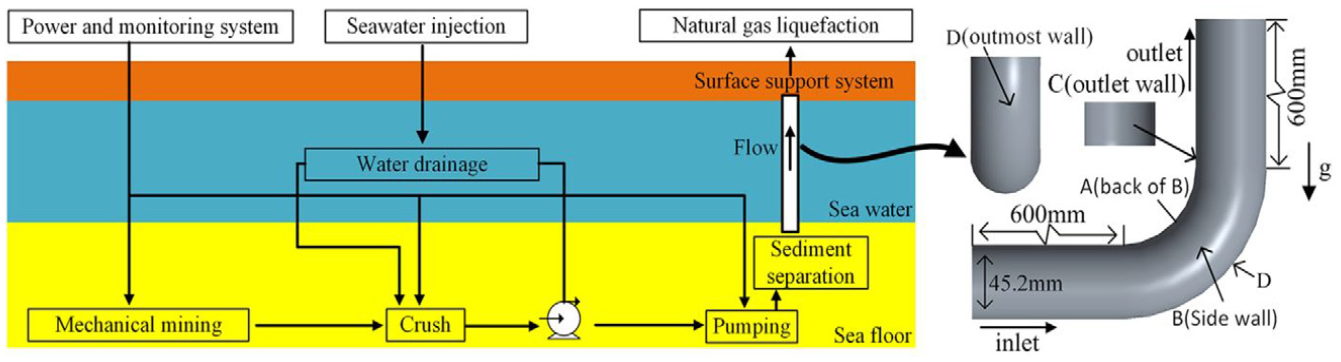
Diagram of the solid fluidization process and the elbow.
Therefore, different from other erosion environment in pipe, there is three-phase flow of hydrate–water–sand in the process of solid fluidization. The geometry of the elbow mainly refers to the experiment model proposed by Balakin et al. 22 In such case, the diameter of the elbow is 45.2 mm and the fillet is 90°. Moreover, the vertical length and horizontal length of pipe are both 600 mm for the purpose of making sure that the flow is completely developed.
Computational mesh
As already known, the mesh generation is a very important step for the numerical simulation and it can further affect the accuracy of the results and the computational time obtained. Figure 2 shows the segmental computational grid employed in this article. The process of grid generation can be conducted through three steps. The first step refers to refining the grid on the plane which is quite normal to the flow direction. The second step is known as applying a proper mesh to the cross-area plane. Finally, the last step is deemed as choosing the appropriate grid which can truly reflect the phenomena of the flow with less time spent on simulation. For the purpose of guaranteeing the accurate results obtained from the computation, the number of boundary layer larger than eight-layer grids, elbow mesh refinement, and the hexahedral unstructured mesh are consequently generated in the computational domain.

Computational mesh.
In such case, the grids with 362,064; 1,011,582; and 1,793,376 elements are adopted for testing the independence of grid. The results obtained from the grid independent test for different tangent planes are shown in Figure 3. When the number of grid elements is 1,011,582, the velocity along the cut path is consistent with the grid elements whose number is 1,793,376. Thus, for the purpose of saving computation resources and balancing computational economy and prediction accuracy, the grid elements of number 1,011,582 are employed to conduct subsequent simulations.

Grid verification.
Mathematical theory
Liquid phase model
The Navier–Stokes equations are adopted in this article, and then, both the continuity equation and momentum equation can be expressed as follows:
For the water phase, the equation is expressed as follows


The equation on the stress tensor is given as follows

For the hydrate phase, the equation is expressed as follows


The equation on the stress tensor is given as follows

where subscripts l and h represent water-phase and hydrate-phase, respectively; α refers to the volume fraction of water or hydrate; ρ denotes the density;
Turbulence model
It is of great importance to choose turbulence model for a specific simulation. The selected turbulence model is established on the basis of the computational demands and decently accurate predicted flow phenomenon proposed by Xie et al. 23 In addition, the re-normalization group (RNG) k–ε is widely employed to deal with the flow turbulence in elbow erosion.14,24,25 Then, the equations of the model are expressed as follows


where subscript m represents the mixing of water and hydrate; GK refers to the turbulent kinetic energy generated by laminar velocity gradient; σk and σε denote the turbulent Prandtl numbers, respectively, C1 = 1.42, C2 = 1.68. As for Sε and Sk, they are the source terms which are determined by the respective discrete phase.
Turbulent viscosity is expressed in the equation as follows

where Cμ refers to a constant that is equal to 0.09.
Disperse phase model
The Lagrange algorithm is employed for predicting the trajectories of particles of discrete phase by employing equilibrating particle stresses. This force balance can be expressed in the equation as follows


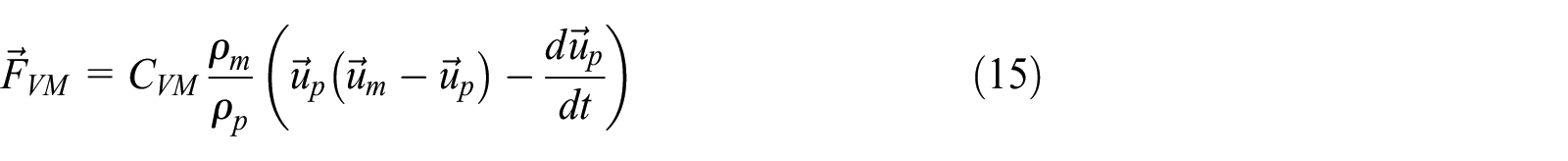
where
Coupling between the continuous phase and the discrete phase
The continuous phase first influences the discrete phase via drag and turbulence, and then, the particles in turn influence the flow through the reduced mean momentum and turbulence. In addition, the two-way coupling is employed to solve this interaction between these phases. Moreover, the discrete phase is taken into account by equations (2), (5), (7), and (8).
As for momentum coupling, the momentum exchange between the discrete phase and continuous phase is computed when the discrete phase passes through each control volume. The exchange is computed by the equation as follows

where Mp refers to the mass flow rate of the particles and
As for turbulence coupling, the continuous phase velocity is composed of two elements in turbulent flow—the mean velocity and the random fluctuation velocity. Among them, the latter influences the discrete phase trajectories. In this article, the influence imposed by turbulence on the discrete phase is considered by employing the DRW model. The fluctuation velocity, which follows a distribution of Gaussian probability, can be computed by employing the following equation

where
If it is supposed that the local turbulence is isotropic, then the calculation on the local root mean square value of the velocity fluctuation can be conducted by employing the local turbulent kinetic energy of the flow field

Two-way turbulence coupling enables the change of effect in turbulent quantities because of particle damping and turbulence. For the purpose of taking this effect into consideration, the terms of particle source are included in the RNG k–ε model, which are in equations (7) and (8), respectively.
Equations of wall collision and rebound
Arabnejad et al. 26 proposed that the hardness of particle plays a significant role in the erosion degree. It is known that the Brinell hardness of the hydrate is 2, the steel is about 140, and sand is about 550. It can be seen that the hardness of sand is about 275 times higher than that of hydrate, and therefore the effect of hydrate impinging on the pipe wall can be neglected. However, the rebound of sand particles after impinging the pipe wall can impose a great effect on the trajectories of particles. Moreover, the velocity of sand particle can be subdivided into the normal velocity and the tangential velocity and it can also be described appropriately, as what was proposed by Grant and Tabakoff. 27
The schematic diagram of particle impacting pipe wall is shown in Figure 4.

Transform of particle impacting the wall.
The velocity ratios of the normal and the tangential before and after collision can be expressed by the equations as below


where subscripts N and T refer to the normal and tangential, respectively. The subscripts 1 and 2 denote the velocity before and after collision, respectively. up indicates the tangential velocity of sand particle, vp represents the normal velocity of sand particle, and θ shows the impact angle.
Erosion model
Many erosion models have been proposed by predecessors. The model selected by Grant and Tabakoff 27 matches well with experimental tests and it is expressed by the equation as follows


The function of the impact angle can be expressed as follows

where ER refers to the erosion rate of elbow; N denotes the number of sand particles which impinge the wall; mp indicates the mass flow rate of sand particles; Aface represents the calculation unit possessed by the area of the wall; superscript b(v) refers to the function of the relative velocity and its value of 2.41 is adopted in this article; C(dp) denotes the function of sand particle; B indicates the Brinell hardness of the target material.
Boundary conditions
Velocity-inlet and pressure-outlet are set as the boundary conditions. For the purpose of guaranteeing the stabilization of discrete phase, more than 30,000 sand particles were uniformly injected into pipe and then the initial velocity of particles is the same as that of the continuous phases. In addition, the hydrate volume ranges from 5% to 30.4% and the percentage of the sand particle volume is about 1%. Moreover, the roughness height is set as 10 μm and the roughness constant is set as 0.5. Furthermore, the wall boundary is “reflect” and the outlet is “escape” and the second-order upwind format is employed for the others. The second-order upwind scheme is adopted for the interpolation to ensure accuracy. The turbulence intensity can be obtained by the equation as follows


where ρm refers to the liquid density; u denotes the flow velocity; D indicates the pipe diameter; μm represents the dynamic viscosity.
The simulation procedure
The SIMPLE algorithm is employed for the calculation of the pressure and velocity in the pipe for the purpose of obtaining more accurate data. In the process, the RNG k–ε turbulent model and discrete phase model (DPM) are established to reflect the fluctuation of continuous phases and discrete phase. Each time the calculation of continuous phases are conducted in five steps, one-step calculation of discrete term is finished. The convergence of residual for the steady simulation is less than 10−6 and a case is calculated for as long as about 8 h. The CFD simulations under different conditions can be described in detail in Table 1.
CFD simulation cases.

CFD: computational fluid dynamics.
Verification of the flow
Verification conducted for the flow model of water–hydrate phase
Under the condition that volume of sand particles is low, the effects imposed by discrete phase on characteristics of continuous phases can be neglected. The experiment carried out by Balakin et al. 22 is adopted to verify the accuracy of the flow model. The hydrate former which is widely used in the experiment is trichlorofluoromethane CCl3F (Freon R11), which is known for low solubility in water. The Freon R11 hydrate is stable in the temperature range at 266–281 K and the pressure range at 0.1–0.13 MPa, as what was proposed by Wittstruck et al. 28 In addition, the process of hydrate formation can be expressed by the equation showing chemical reaction as follows

The entire loop was designed in an environment-controlled cabinet in which the fluids is kept at low temperature. As for the basic parameters, they are shown in Table 2 as follows.
Experimental conditions from Balakin et al. 22

The experiment versus simulation results are shown in Table 3.
Comparison between results obtained from experiment and simulation.

On the whole, the deviation between the simulation and experiment is less than 3%. The RNG k–ε turbulent model, which is established based on the Eulerian flow model can well describe the characteristics of water–hydrate phase.
Validation conducted for the model of water–sand phase erosion
For the purpose of verifying the erosion model, the two-phase flow experiment of water–sand carried out by Zeng et al. 29 is employed. The carbon steel array electrodes of X65 pipeline with an exposed area of 5 mm × 6 mm for each were used in the experiment. The experiment lasted 14 h and the weight loss of each electrode was further measured for the determination of the total E–C (erosion–corrosion) rate.
The experimental parameters are shown in Table 4.
Experimental conditions from Zeng et al. 29

Figure 5 shows scatter curve of the maximum erosion rate possessed by elbow between experiment and simulation. It is shown in the study that the erosion rate gradually increases along with the increase in plane angle. In addition, the deviation obtained from the maximum erosion rate in 80° plane is below 8%. Moreover, the deviation obtained from the 70° plane is about 20% and all the deviation obtained from other planes exceed 30%. The deviation between E/CRC model and the simulation decreases along with the increase of elbow angles. 14 Based on the experimental condition and the maximum erosion positions, it is observed that the elbow erosion mainly occurs when the angles are larger than 50° and therefore, the deviation between E/CRC model and the simulation is acceptable. However, because of the low angles, the random motion of particles is known as the main cause of erosion which accordingly triggers the difference of erosion between E/CRC model and the simulation. Due to the fact that no corrosion is taken into account in the CFD simulation in comparison with the experiment, the rates of experimental erosion obtained are larger than that obtained from the simulation and E/CRC model. It is also shown that the erosion rates with and without considering the effect of corrosion are different. Therefore, the effect of corrosion will be considered in studies conducted in the future. However, the variation trends obtained from experiment and the simulation are similar. In the field, the failures of pipeline occur mostly in the pipe zones which are mostly impacted. The deviation in maximum erosion rate of elbow between the simulation and the experiment is 8%, which is within an acceptable range. Therefore, it is finally concluded that the simulation can effectively predict the most severely impacted location of the elbow.
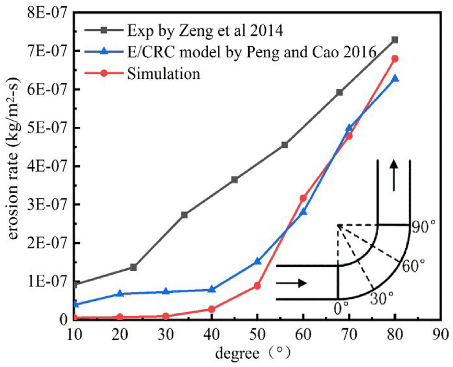
Comparison of results from experiment and simulation.
Results and discussion
Case 1: effect of hydrate on erosion
The movement of particles in elbow are in the control of three main forces, namely the drag force, the inertia force of particle, and the secondary flow. The inertia force, which is regarded as the essential attribute of the particle that has close relationship with the mass, leads the particles to move in tangential direction. The drag force is closely related to the viscosity of the flow which can be controlled by volume friction of hydrate as mentioned above in this article. Under the influence of the centrifugal force in elbow, the fluid flow from outside wall to inside wall and it is known as the secondary flow. Actually, the final erosion of elbow is caused by the interactions of these forces.
The basic parameters included in case 1 is shown in detail in Table 1. Figures 6 and 7 show the effect of hydrate on the properties of Reynolds number, flow density, and viscosity possessed by the fluid. It can be observed that the flow density and viscosity increase linearly and exponentially along with the increase of hydrate volume. However, the Reynolds number increases first and then decreases linearly. In addition, when the hydrate volume is 5%, the Reynolds number arrives at the maximum value of 182,047 while the pipe erosion rate is as high as 1.02e−6kg/m2/s. Moreover, the variation tendency shown by Reynolds numbers is the same as that of the pipe erosion rate. Besides, it is worth noting that the higher Reynolds number indicates the larger impinge energy of the flow. Therefore, it is of vital importance for prolonging pipe life in solid fluidization by controlling the volume friction of hydrate.
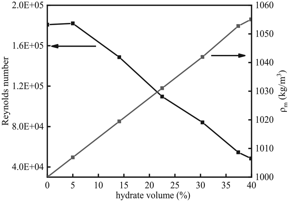
The effect of hydrate volume on Reynolds number.
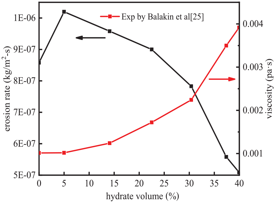
The effect of hydrate volume on erosion rate.
Figure 8(a) shows the trajectories of particles for hydrate of different volumes. According to the smooth motion streamlines of particles, it is obtained that the inertia force is stronger than the secondary flow, which leads the particles impinge on the outmost wall (zone D) as shown in Figure 8(b). When hydrate volume is larger than 5%, the viscosity of the continuous phase increases significantly and accordingly the adhesion between fluid and particles increases as well. Therefore, the quantity of particles impinging on the zone D decreases, which results in a decrease of the erosion rate. It can be finally concluded that the erosion degree on zone C is more severe than that of zone A/B. The erosion zones A/B and C mainly results from the secondary flow, however, the secondary flow is not deemed as the dominant force in comparison with the inertial force. Meanwhile, the impact angle of zone C is larger than that of zone A/B, and therefore, erosion in zone C is more severe than that in zone A/B. Along with the increase of hydrate volume, the intensity of secondary flow decreases gradually and the impact angle of zone C decreases as well. Consequently, the erosion rate of zone C decreases along with the increase of hydrate volume.

The effect of hydrate volume on erosion: (a) sand particle trajectory and (b) contour of erosion rate.
Case 2: effect of R/D rate on erosion
Table 1 shows the basic parameters of case 2. The erosion rates for different R/D rates are presented in Figure 9. The erosion rate decreases along with the increase of R/D rate. Furthermore, when the curvature is 3 D and 3.5 D, the erosion rate is almost the same, and therefore the effect imposed by increased R/D rate on reducing the erosion rate of the elbow is limited when curvature is larger than 3 D.
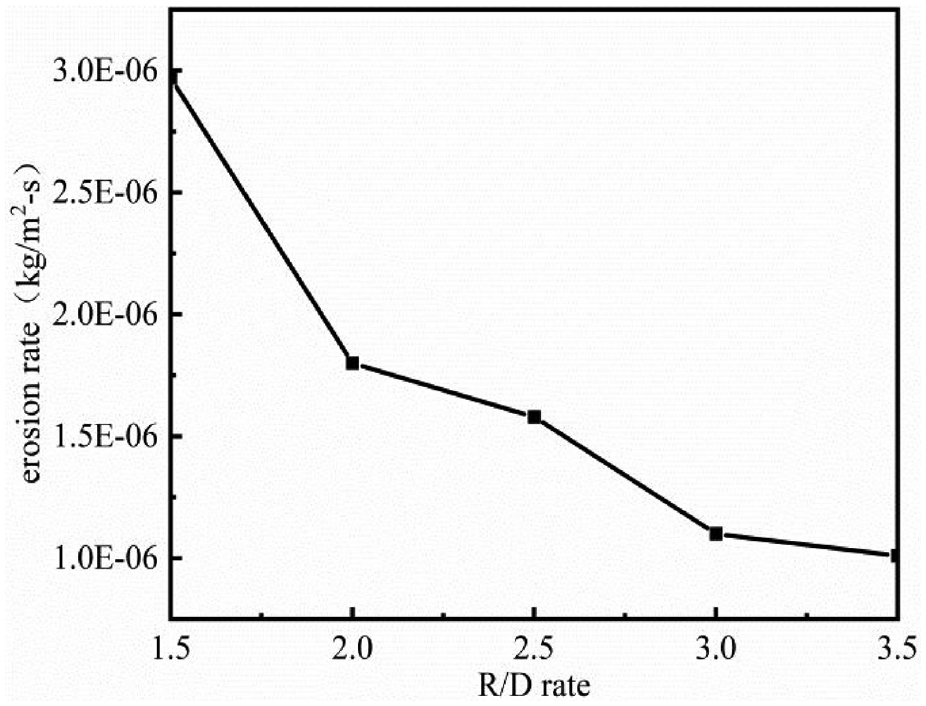
The effect of R/D rate on erosion rate.
Figure 10(a) shows the trajectories of particles for different R/D rates. It is quite obvious that the particles flow easily and smoothly for larger R/D rate. Along with the increase of R/D rate, the intensity of secondary flow gradually weakens. As shown in Figure 10(b), the contours of erosion rate for different R/D rates are presented. As expected, the erosion rate decreases along with the increase of R/D rate. This phenomenon is mainly caused by the longer pathway for large curvature elbow, which well adapts the direction mutation of fluid in comparison with the small curvature.
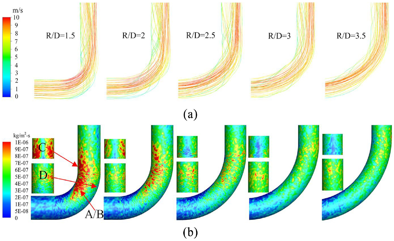
The effect of different R/D rates on erosion: (a) trajectory of sand particle and (b) contour of erosion rate.
Moreover, the secondary flow is known as the main force triggering the serious erosion in zone A/B and zone C when R/D = 1.5. When R/D is larger than 2.5, the distribution of erosion is mainly concentrated on zones A/B and D and the erosion area is much smaller than R/D = 1.5. Additionally, the area of high erosion rate on zone A/B is larger than that of zone C, especially for large R/D rates. Actually, this phenomenon is mainly caused by the decreased impact angle on zone C.
Figure 11 shows the velocity vector on angle slices from 10° to 80°, where R/D rate is equal to 1.5 and 3.5 D. The secondary flow forces the movement of the solid particles toward the outer wall (zone D) and it is also known as the main reason for erosion on zone A/B and zone C. In the simulation of the same conditions, R/D = 3.5 can reduce not only the intensity of secondary flow but also the erosion rate.
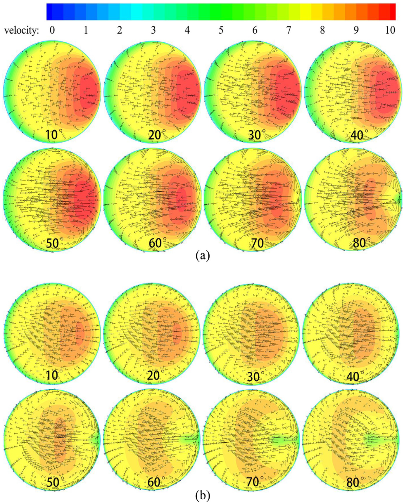
Cross-section velocity vector: (a) cross-section velocity vector when R/D = 1.5 and (b) cross-section velocity vector when R/D = 3.5.
Case 3: effect of flow velocity on erosion
Table 1 shows the basic parameters of case 3. As for Figure 12, it shows the effect of different velocities on erosion rate. In addition, it is observed that the erosion rate increases exponentially along with the increase of velocity, and this result is consistent with the experiment conducted by Zhang et al. 3

The effect of velocity on erosion rate.
Figure 13(a) shows the trajectories of sand particles for different velocities. It is observed that the fluctuations of particles mostly focus on zones A/B and C, as well as the erosion. Moreover, a small part of particles impose their impact on the outmost wall, which accordingly leads to slight erosion on zone D. Therefore, the variation of flow velocity will not change the erosion zone obviously as shown in Figure 13(b). Determined by the Reynolds number, it is concluded that the higher the flow velocity, the greater the turbulence intensity and the erosion rate.

The effect of velocity on erosion: (a) trajectory of sand particle and (b) contour of erosion rate.
Case 4: effect of particles diameter on erosion
Table 1 shows the basic parameters included in case 4. The effect of particles diameter on erosion rate is shown in Figure 14. It is observed that the erosion rate increases from 2.97e−6 to 1.57e−5 kg/m2/s as the diameter of particles increases from 60 to 480 μm.
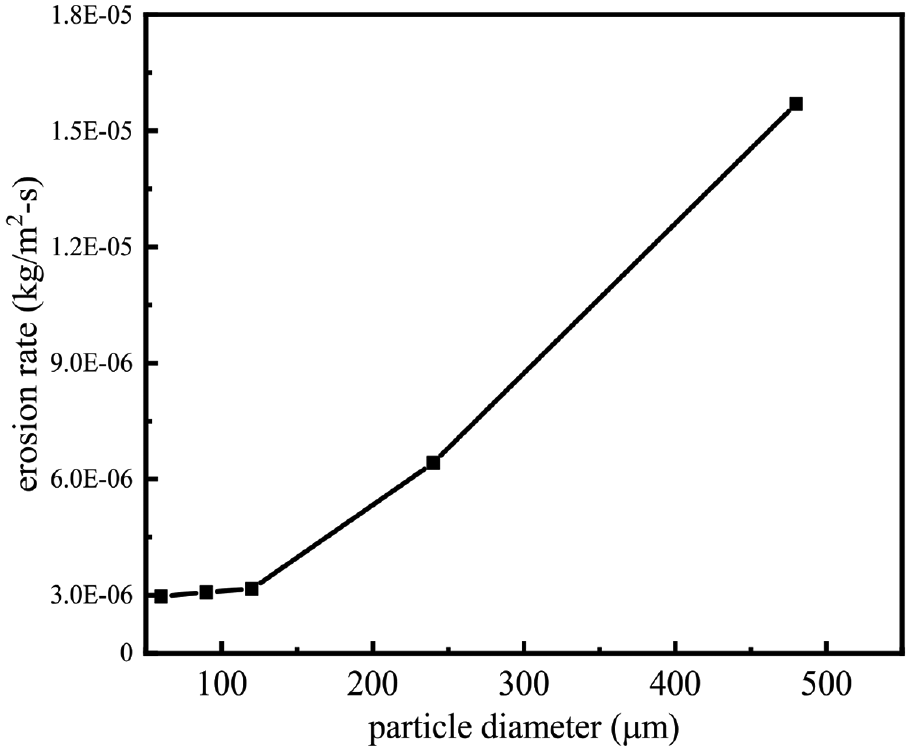
The effect of particle diameter on erosion rate.
Figure 15(a) shows the trajectories of particles shown by particles of different diameters. It is quite obvious that the fluctuations of particles in elbow are stronger when the diameter of particles is 60 μm in comparison with the particles with the diameter of 480 μm. For the particle with large diameter, the energy of inertial force generated is enough to overcome the constraint of the drag force and secondary flow. Therefore, with the diameter of particles increasing, the main zone of erosion changes from zone A/B to zone D, which is shown in Figure 15(b). Therefore, it is important to control the particle size for the purpose of reducing erosion concentration on the outmost wall (zone D).

The effect of particle diameter on erosion: (a) trajectory of sand particle and (b) contour of erosion rate.
Case 5: effect of Stokes number on erosion
Table 1 shows the basic parameters included in case 5. The Stokes number, which refers to the ratio of particle relaxation time to fluid characteristic time, can reflect the ratio between inertia force and drag force of particle. The formula is expressed as follows

where ρp refers to sand particle density, dp denotes the diameter of particle, u indicates the flow velocity, and μ represents the viscosity of continuous phase.
For the purpose of describing the effect of Stokes number on transformation of erosion zone, the transformation of the erosion zone is divided into three processes (T1, T2, and T3) as shown in Figure 16. Particles with the sizes of 60, 180, and 420 μm are representatives of each process, which is shown in Figure 17. As for a specific elbow, the main erosion zone changes from the initial zone A/B to the final zone D as the particle diameter increases to the threshold value. Moreover, when the diameter of particle is small, the drag force would be known as the dominating force and the erosion mainly results from the secondary flow. On the contrary, the inertia force then becomes the dominating force when the diameter of particle arrives at a certain value.

The erosion rate under different diameters and R/D rates of particle.

The transformation of the erosion zone.
It is quite obvious that the same Stokes number on elbow reflects the phenomena of different erosions. Therefore, only taking into account the Stokes number is unable to reflect the universality in engineering.
Analysis of the sensitivity of parameters
According to the range of parameters analyzed in this article, the effect imposed by the volume of hydrate on erosion rate is much smaller than that of other parameters. Therefore, the parameters including flow velocity, particle diameter, and R/D rate are chosen for sensitivity analysis and the erosion rate is taken as a criterion. Given no interactions is available among factors, values of three levels are then taken into consideration.
Table 5 shows the orthogonal experiments of flow velocity, R/D rate, and the diameter of particle. In the table, Li refers to the arithmetic mean of the erosion rates at the factor level (i = 1–3) and R indicates the Max – Min.
Orthogonal experiment.

Based on the Max – Min of different factors, the effect imposed by the order of parameters on erosion rate can be given as follows: velocity > particle diameter > R/D rate.
Conclusion
In the study, the Euler with RNG k–ε turbulent model is applied to treat the hydrate and the water as continuous phases and the Lagrange is employed to simulate the trajectories of particles. Then, relevant analysis is conducted on the effects imposed by hydrate volume, R/D rate, flow velocity, and diameter of particles on elbow erosion. In terms of the organization of the article, it is mainly divided into four parts including experimental verification, grid verification, factors analysis, and orthogonal experiment. Moreover, the conclusions can be summarized as follows:
The hydrate volume is able to impose its effect on flow viscosity and Reynolds number. The variation trend of erosion rate is consistent with that of Reynolds number, and the Reynolds number as well as the erosion rate reaches the maximum when hydrate volume is 5%.
The effect imposed by the increased R/D rate is limited on mitigating the erosion rate when R/D rate is larger than 3. When the R/D rate is large, the erosion zone of the elbow becomes more uniform and the main zones of erosion change from zone A/B to zones A/B and D.
The erosion rate increases exponentially along with the increase of flow velocity. As for particle of small size, the main erosion tends to occur in side wall (A/B) under the influence of secondary flow. However, for large size particle, the erosion tends to occur in the outmost wall (D) because of the inertial force.
With different R/D rates, the same Stokes number is able to reflect the different dynamic transformations of the maximum erosion zone. However, along with the increase of Stokes number, the erosion zone of the elbow will eventually stabilize at zone D.
Based on the orthogonal experiment, the flow velocity is known as the most sensitive factor among diameters of particles and R/D rates.
Footnotes
Declaration of conflicting interests
The author(s) declared no potential conflicts of interest with respect to the research, authorship, and/or publication of this article.
Funding
The author(s) received no financial support for the research, authorship, and/or publication of this article.