Sage Journals: Discover world-class research

Abstract

A method of water injection to flow field using distributed holes on the suction surface of hydrofoil is presented in this article to control cavitation flow. Modified renormalization group k–ε turbulence model is coupled with full-cavitation model to calculate periodical cavitation patterns and the dynamic characteristics of the NACA66(MOD) hydrofoil. Water injection is found to be highly effective for cavitation suppression. The cavitation suppression effect of distributed regulation of jet holes and porosities along three-dimensional spanwise hydrofoil is also investigated. The appropriate porosities of single row spanwise jet holes and optimal jet position of double row jet holes are revealed for both cavitation suppression and good hydrodynamic performance. Double row jet holes setting in forward trapezoidal arrangement shows great potential for cavitation suppression and hydrodynamic performance. This research provides a method of water injection to flow field to actively control cavitation, which will facilitate development of engineering designs.

Keywords

Active control sheet/cloud cavitation jet porosity jet position hydrodynamic performance

Introduction

Cavitation phenomenon reduces hydraulic performance and creates vibration and noise, which seriously affects the safety and stability of system operation.¹,² The configuration of cavitation can be divided into five categories: bubble cavitation, sheet cavitation, cloud cavitation, super cavitation, and vortex cavitation. Considering the intense unsteady flow characteristics of cavitation, cloud cavitation is the most harmful to equipment. Previous research has shown that the re-entrant jet is responsible for cloud cavitation shedding. Instantaneous high pressure can occur in the position of collapsing bubble, producing a strong shock wave which causes damage to the surface of the blade and forms cavitation erosion.^3
–7

To suppress or even control cloud cavitation phenomenon, numerous scholars have adopted the passive control method.⁸ The cavitation flow field is restricted by setting obstacles in the suction surface of the hydrofoil in order to suppress cloud cavitation shedding.^9
–15 However, obstacles arranged in the hydrofoil may cause a decrease in the lift-to-drag ratio. Moreover, it is difficult to meet variable working condition regulation processes once a definite obstacle is set in the surface of the hydrofoil.

Arndt et al. carried out cavitation experiments based on active flow control technology,¹⁶ in which air jet holes were arranged at the leading edge of the blade.¹⁷ It was found that jet air can play the role of an air pillow to improve the pressure fluctuation on the blade of the cavitation zone and effectively decrease the corrosion caused by cavitation. Mäkiharju et al.¹⁸ injected non-condensable gas in the downstream cavitation zone of the vertices of the delta wing and the recirculation zone in the middle of the cavitation body. They found that a small amount of gas injected into the middle of the cavitation zone has little effect on cavitation suppression. To minimize the cavitation phenomenon, Hassanzadeh et al.¹⁹ applied wall injection to the diesel injector to control boundary layer separation inside the injector. Timoshevskiy et al.²⁰ used a continuous tangential liquid injection supply through a spanwise slot in the surface of a scaled-down model of a high pressure turbine guide vanes to achieve favorable and efficient flow manipulation. This process was found to reduce the amplitude substantially, and even totally suppressed periodic cavity length oscillations and pressure pulsations, especially in systems with developed cavitation rather than cavitation-free and cavitation inception cases.

In this article, NACA66(MOD) hydrofoil is used as the research object. Based on active flow control technology, specific inner and surface hydrofoil structures (Figure 1) are designed to make the fluid flow into the mainstream zone along the setting channel for the purpose of weakening the intensity of re-entrant jet and further suppressing cloud cavitation. According to the intensity of cavitation, the injection velocity can be adjusted to alter cavitation flow in various cavitation conditions. The setting channel from inlet pipe to injection holes on the surface of the hydrofoil forms the internal flow field. External flow field around the hydrofoil is simulated on the basis of the modified renormalization group (RNG) k–ε turbulence model with density correction, combined with the full-cavitation model used by Singhal, to investigate the cavitation flow field. This article is focused on the influence of jet hole distribution and spanwise porosities on the hydrofoil surface on cavitation suppression and hydrodynamic performance.

Figure 1.

3D schematic representation of modified NACA66(MOD).

Physical model and numerical method

Governing equations

The homogeneous flow model or two-phase flow (inhomogeneous flow) model is commonly used in the calculation of cavitating flow. In the homogeneous flow model, the mixture of vapor liquid two-phase flow is regarded as a homogeneous medium, and the weighted average values of the two-phase parameters are taken as the corresponding parameters of homogeneous flow. The vapor liquid two-phase flow is thus treated as a single-phase flow with average fluid characteristics, meaning that the vapor phase and the liquid share the same velocity field, pressure field, and turbulent flow field. In the inhomogeneous flow model, each fluid in the flow field is independent and has its own governing equation, and the interaction between the phases cannot be neglected.²¹ For the calculation of cavitating flow in the two-phase flow model, mass transfer, momentum transfer, and slip coefficient between vapor and liquid phases should be taken into account. The two-phase flow is difficult to solve, while the homogeneous flow model is simpler and more economical than the inhomogeneous flow model. The homogeneous flow model has thus been favored by many scholars studying cavitating flow.^22
–24 And in this study, the homogeneous model is adopted.

The following governing equations will be used in cavitation flow field simulation.

The continuity equation

\frac{\partial ρ_{m}}{\partial t} + \frac{\partial (ρ_{m} u_{j})}{\partial x_{j}} = 0

(1)

The momentum equation

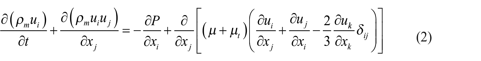
\frac{\partial (ρ_{m} u_{i})}{\partial t} + \frac{\partial (ρ_{m} u_{i} u_{j})}{\partial x_{j}} = - \frac{\partial P}{\partial x_{i}} + \frac{\partial}{\partial x_{j}} [(μ + μ_{t}) (\frac{\partial u_{i}}{\partial x_{j}} + \frac{\partial u_{j}}{\partial x_{i}} - \frac{2}{3} \frac{\partial u_{k}}{\partial x_{k}} δ_{i j})]

(2)

where ρ_m is the mixture density, u is the mixture velocity, P is the mixture pressure, µ is the mixture laminar viscosity, and µ_t is the turbulent viscosity. The subscripts (i, j, and k) denote the directions of the Cartesian coordinates. ρ_m and µ are defined as

ρ_{m} = ρ_{l} (1 - α_{v}) + ρ_{v} α_{v}

(3)

μ = μ_{l} (1 - α_{v}) + μ_{v} α_{v}

(4)

where ρ_l is the liquid density, ρ_v is the vapor density, α_v is the vapor void fraction, and µ_l and µ_v are the liquid and vapor dynamic viscosities, respectively.

Cavitation model

The cavitation model is based on the full-cavitation model developed by Singhal.²⁵ This model explains all first-order effects of cavitation, including phase transition, bubble dynamics, turbulent pressure fluctuation, and non-condensable gases. It has the ability to solve the effects of multiphase flow or multiphase material transport, vapor phase and liquid phase slip velocity, as well as the thermodynamic effect and compressibility between vapor and liquid phases. At the same time, the full-cavitation model is always adopted with mixed phase model, and with or without velocity slip. This model is also applicable to single-phase equations. The government equation of the full-cavitation model is

\frac{\partial}{\partial t} (ρ_{m} f_{v}) + \frac{\partial}{\partial x_{j}} (ρ_{m} u_{j} f_{v}) = R_{e} - R_{c}

(5)

where the source term R_e represents the evaporation rates and the sink term R_c represents condensation rates. The evaporation and condensation terms are defined as

R_{e} = C_{e} \frac{\sqrt{k}}{τ} ρ_{l} ρ_{v} {[\frac{2}{3} (\frac{P_{v} - P}{ρ_{l}})]}^{\frac{1}{2}} (1 - f_{v} - f_{g})

(6)

R_{c} = C_{c} \frac{\sqrt{k}}{τ} ρ_{l} ρ_{l} {[\frac{2}{3} (\frac{P - P_{v}}{ρ_{l}})]}^{\frac{1}{2}} f_{v}

(7)

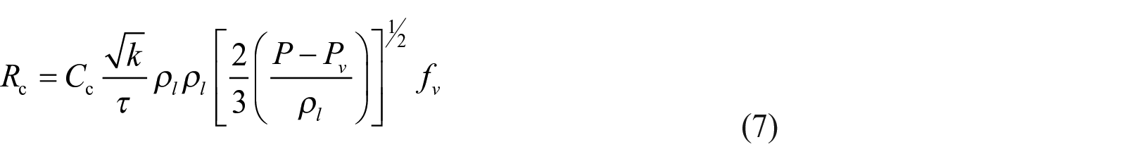
where k represents the turbulent kinetic energy and τ (= 0.07349 N/m) represents the surface tension coefficient; the empirical factors, C_e and C_c, have the following values: C_e = 0.02 and C_c = 0.01; and f_v is the vapor mass fraction and f_g is the non-condensable gas mass fraction.

Turbulence model

Studies have shown that the cavity shedding frequency of calculated results adopted by the standard RNG k–ε turbulence model is much greater than the experimental results. However, the calculated results using RNG k–ε turbulence model with density correction demonstrate strong correspondence with the experimental results.²⁶ Therefore, the modified RNG k–ε turbulence model is used in this article for the calculation of cavitation around the NACA66(MOD) hydrofoil.

The transport equations for the RNG k–ε model are as follows

\frac{\partial}{\partial t} (ρ k) + \frac{\partial}{\partial x_{i}} (ρ k u_{i}) = \frac{\partial}{\partial x_{j}} (α_{k} μ_{t} \frac{\partial k}{\partial x_{j}}) + G_{k} + G_{b} - ρ ε - Y_{M} + S_{k}

(8)

\frac{\partial}{\partial t} (ρ ε) + \frac{\partial}{\partial x_{i}} (ρ ε u_{i}) = \frac{\partial}{\partial x_{j}} (α_{ε} μ_{t} \frac{\partial ε}{\partial x_{j}}) + C_{1 ε} \frac{ε}{k} (G_{k} + C_{3 ε} G_{b}) - C_{2 ε} ρ \frac{ε^{2}}{k} + S_{ε}

(9)

In the RNG k–ε model, G_k and G_b are the generation of turbulence kinetic energy due to the mean velocity gradients and buoyancy, respectively. Y_M represents the contribution of the fluctuating dilatation in compressible turbulence to the overall dissipation rate, and α_k and α_ε represent the inverse effective Prandtl number for k and ε, respectively.

The modified RNG k–ε turbulence model considered the compressibility of the two-phase flow. The turbulent viscosity is modified by

μ_{t} = f (ρ) C_{μ} \frac{k^{2}}{ε}

(10)

f (ρ) = ρ_{v} + {(1 - α_{v})}^{n} (ρ_{l} - ρ_{v})

(11)

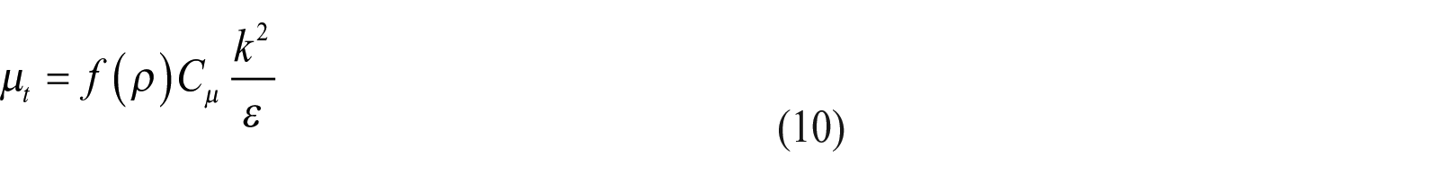
where ε is the turbulent dissipation rate, the model constant C_µ = 0.085, and the turbulent viscosity is limited by n. The value of n has been taken as 10 in Coutier-Delgosha et al.,²⁷ but no corresponding explanation has been provided. As seen in Figure 2, when vapor content is the same, the influence of turbulent flow field on the calculation of cavitating flow can be reduced by introducing density correction function, especially in the vapor–liquid mixing region with small vapor content. For example, if the modified curve n = 3 is introduced, the turbulent viscosity will be reduced by 1/2 when the vapor volume fraction is 30%. This can limit excessive turbulent viscosity in the water–vapor mixing zone at the tail of the cavity.

Figure 2.

Modification of turbulent viscosity with density correction index n.

To obtain good simulation results, the effects of different correction coefficients n on the simulation results are compared. The experiments were carried out by Leroux.²⁸ The pressure fluctuations at the middle chord of the suction side of the hydrofoil under different n are provided in Figure 3. AOA represents the attack angle of hydrofoils. The results show that in the first 0.8 T_cycle, the pressure fluctuations display strong correspondence with the experimental results, and the last 0.2 cycle has a deviation range of 5% to 7%. This error is within an acceptable range, and when the density correction coefficient n = 3, the deviation is the smallest. An appropriate density correction coefficient n brings the simulation results closer to the experimental values, so the value of density correction coefficient n is adopted as 3 in this article.

Figure 3.

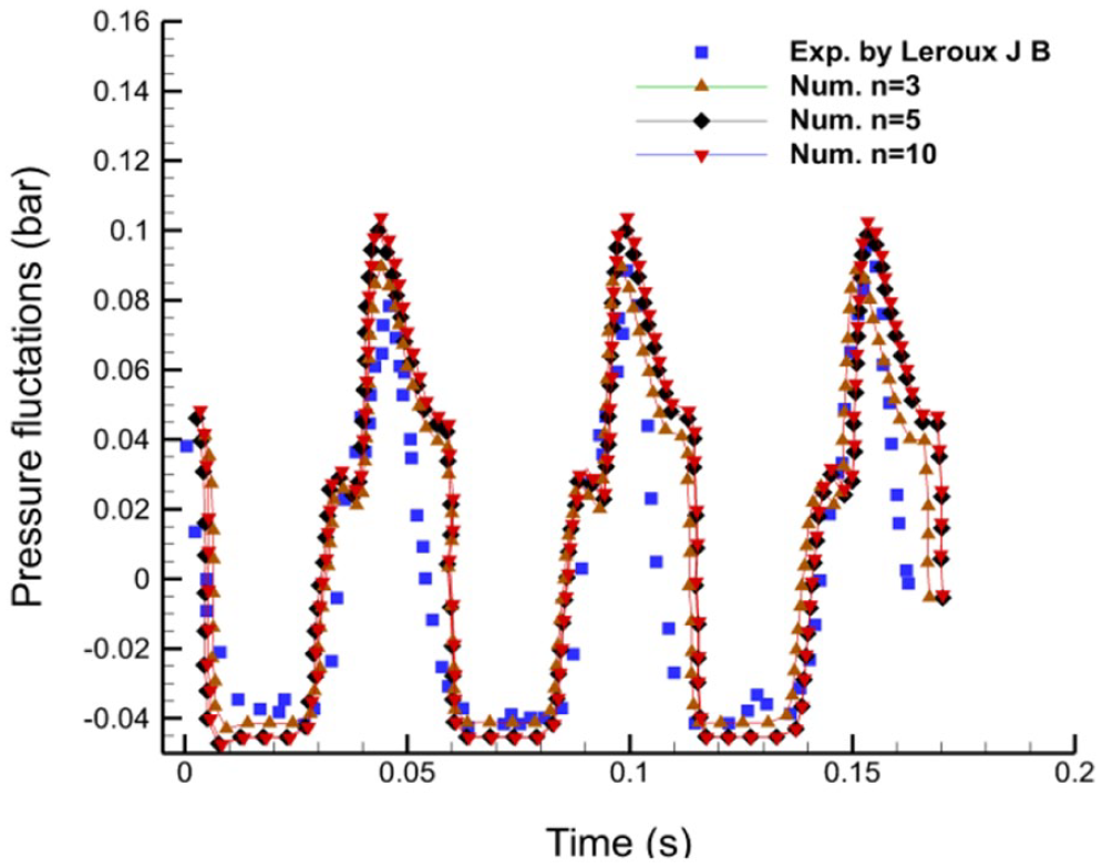
Comparison of pressure fluctuations at mid-chord on the hydrofoil suction side (AOA = 8°, σ = 1.45, V_ref = 5.33 m/s).

Physical model and solving settings

The calculation conditions are consistent with the experimental conditions, and the coordinates of NACA66(MOD) hydrofoil are determined according to Leroux.²⁸ The chord length is 0.15 m, and spanwise length is 0.192 m. The inlet velocity is 5.33 m/s, corresponding to a Reynolds number Re = 8 × 10⁵ based on the reference length of the hydrofoil chord length. The boundary conditions and three-dimensional (3D) computational domain are illustrated in Figure 4. The computational domain has an extent of about 3c upstream from the leading edge and 5c downstream from the trailing edge of the foil (where c is the chord of the hydrofoil). Three mesh resolutions are used for mesh independence test. The chordwise mesh distribution is the same for all three cases according to the mesh generation method in the previous two-dimensional (2D) hydrofoil research.²⁹ The only difference is the number of nodes in the spanwise direction, as shown in Figure 5. Table 1 shows the result of the mesh independence test; while f means shedding frequency of cavity, it can be seen that the differences between the medium and dense resolution meshes can be neglected, and both the predicted cavity shedding frequencies are close to the experimental result. Thus, the medium resolution mesh is adopted for saving computing resources. In order to describe the intensity of jet, the jet flow ratio (JFR) is defined as the ratio of jet velocity and inlet velocity.

Figure 4.

Computational domain and mesh around NACA66(MOD) hydrofoil.

Figure 5.

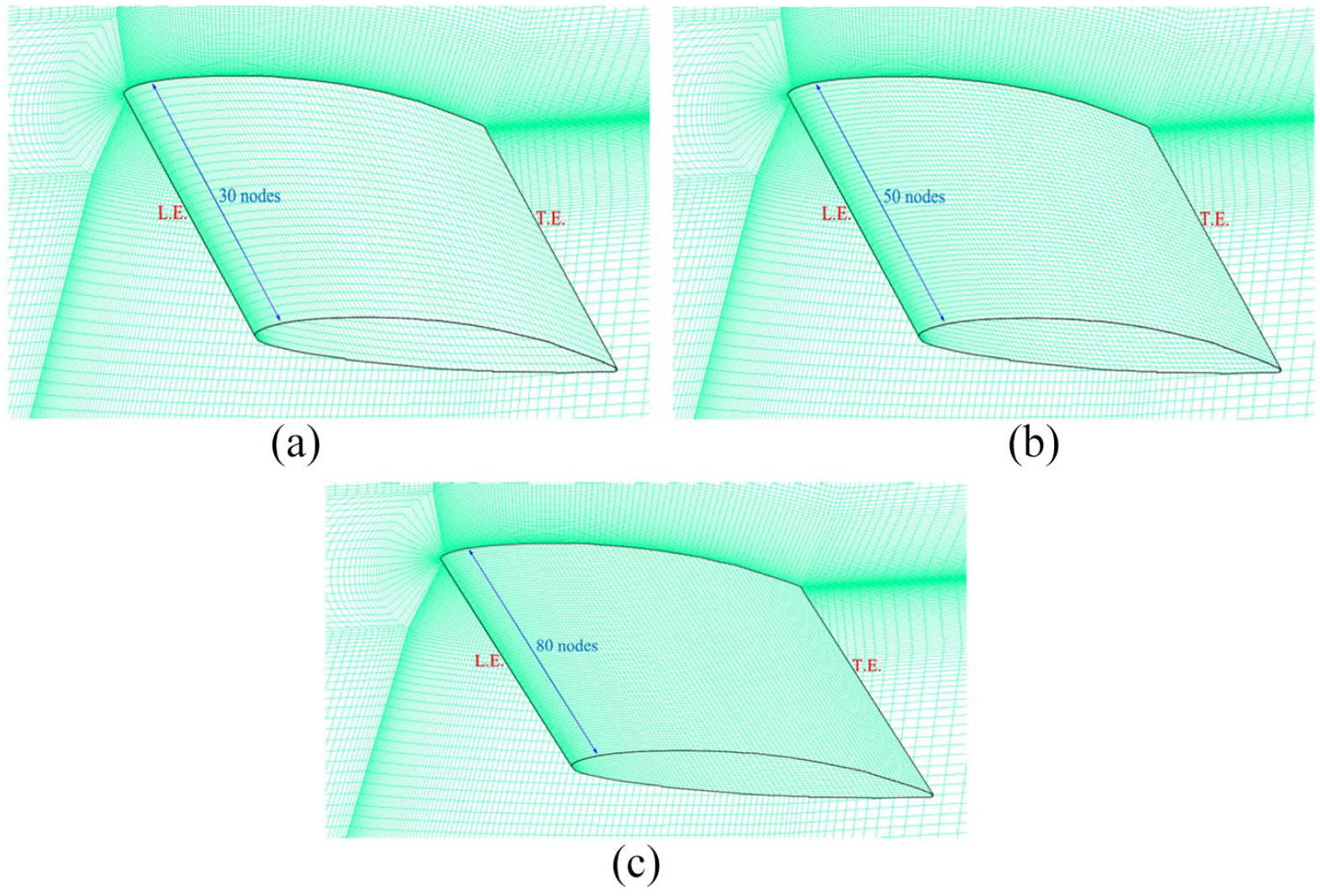
Three cases of mesh around three-dimensional hydrofoils: (a) mesh case 1 (total 1,023,420 nodes), (b) mesh case 2 (total 1,705,700 nodes), and (c) mesh case 3 (total 2,729,120 nodes).

Table 1.

Results of the mesh independence test (AOA = 6°, σ = 1.0, V_ref = 5.33 m/s).

	Mesh resolution	Nodes	C_l	C_d	f /Hz
Case 1	Coarse	1,023,420	0.761630	0.043768	3.32
Case 2	Medium	1,705,700	0.779349	0.062458	3.49
Case 3	dense	2,729,120	0.750746	0.061621	3.49
Experiments	–	–	–	–	3.50

The Semi-Implicit Method for Pressure-Linked Equations-Consistent (SIMPLEC) scheme is used to solve the coupling of velocity field and pressure field. The PREssure STaggering Option (PRESTO) system is then selected for the pressure interpolation with the Quadratic Upstream Interpolation for Convective Kinematics (QUICK) scheme used for the vapor mass fraction transport equation. The time step of unsteady cavitation calculation must meet the Courant–Friedrich–Levy stability criterion. Considering computation time and solution accuracy, the time step is 0.0005 s in this article.

Results and discussion

The Y+ on the suction side of the hydrofoil is shown in Figure 6. As shown, the Y+ value ranges from 18 to 100, which meets the requirements of high Reynolds number model (Y+ ranges from 30 to 300). To verify the accuracy of density modified RNG k–ε model, the pressure coefficients of suction surface of hydrofoil under non-cavitation flow (Figure 7), the frequency of cavity shedding (Table 2) under σ = 1.0, and the shape of cavity in a cycle²⁹ are obtained. All the results of these three aspects are in good agreement with the experiments,²⁸ which indicate that the density modified RNG k–ε combined with the full-cavitation model have a high reliability in simulating steady and unsteady cavitation flow fields. The research in this article is based on this model.

Figure 6.

Contour of Y+ on the suction side of the hydrofoil.

Figure 7.

Comparison of pressure distribution for a non-cavitating flow.

Table 2.

Comparison of cavity shedding frequency (AOA = 6°, σ = 1.0, V_ref = 5.33 m/s).

Calculation methods	M-RNG				RNG	Experiments
Calculation methods	n = 2	n = 3	n = 5	n = 10		Experiments
f /Hz	3.752	3.487	3.523	3.367	3.968	3.5

RNG: renormalization group; M-RNG: density modified RNG k–ε turbulence model.

Previous studies²⁹ have shown that for 2D hydrofoil, under the condition σ = 0.55, when the jet hole is arranged at the vertex position (the top position of suction side of the hydrofoil under a certain AOA; for AOA = 6°, the vertex position is x = 0.25 c) with a jet angle of θ = 155° on the suction side of the hydrofoil, and with the JFR of 0.3, water injection displays the highest cavitation suppression effectiveness. The best hydrodynamic performance (the maximal lift-to-drag ratio and the minimal cavity stretching frequency) is also maintained under these conditions. In this article, further study of cavitation suppression on 3D hydrofoil is carried out based on the previous research.

Effect of jet holes’ porosity

The effect of jet hole porosity of 3D hydrofoil surface on the cavitation flow control is investigated under conditions of the optimum jet position (x = 0.25 c) and the optimum jet angle (θ = 155°).²⁹ The distribution of the jet hole at different porosities is illustrated in Figure 8. To reduce the workload of mesh generation and the computing demand of multiple grids, the circular holes are simplified into nine evenly spaced holes, which are made up of a rectangular hole and two semicircle holes with the diameter of 2 mm. By adjusting the length of the rectangular hole to change the porosity of the jet hole, the distances between the outside jet holes and the end surface of the hydrofoil are maintained at 5 mm.

Figure 8.

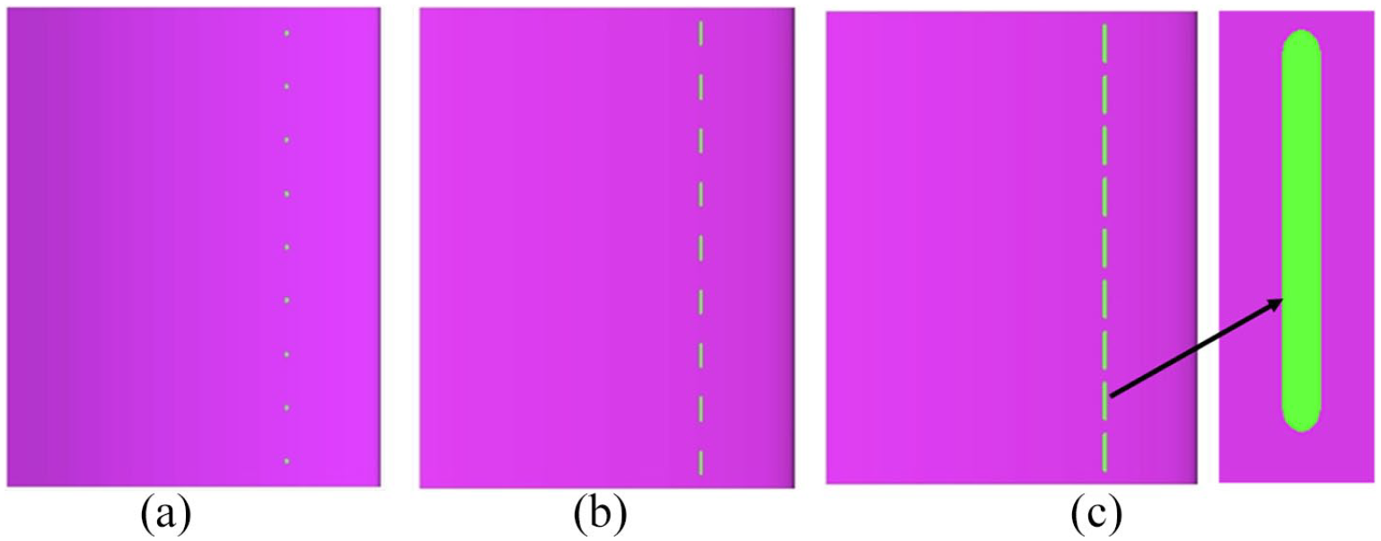
Distribution of jet hole at different porosities, x = 0.25 c, θ = 155°: (a) ϕ = 7.36%, (b) ϕ = 44.86%, and (c) ϕ = 72.99%.

The definition of jet porosity is

φ = \frac{9 \times (S_{rectangular hole} + 2 \times S_{semicircle hole})}{0.002 \times 0.192} \times 100 %

(12)

where S refers to the area of holes.

Numerical simulations of cavitation flow field are carried out for the jet hole porosity of 35.49%, 44.86%, 54.24%, 58.92%, 63.61%, and 72.99%, with JFR of 0.3. The periodic evolution of cavitation shape pattern around the hydrofoil surface and the contours of cavity with vapor volume fraction of 10% are provided in Figure 9, where the jet hole porosity is 0 (no jet hole), 54.24%, 58.92%, and 63.61%.

Figure 9.

Comparison of instantaneous cavity shape at different porosities in a cycle (iso-surface of α_v = 10%), σ = 0.55, AOA = 6°: (a) ϕ = 0.00%, (b) ϕ = 54.24%, (c) ϕ = 58.92%, and (d) ϕ = 63.61%.

As illustrated, the shapes of cavity are closely related to the velocity distribution characteristics of the re-entrant jet. When there is no jet hole, the re-entrant jet occurs at the trailing edge (0.8 c) of the hydrofoil, and, at the same time, the lateral re-entrant jet is generated. When the cavitation develops to a certain stage, the closed cavity in the trailing edge becomes very unstable and two symmetrical concave shapes appear (t = 3/8 T–4/8 T; Figure 9(a)). With the development of cavitation, the area covered by the re-entrant jet and the lateral jet is further expanded and moves toward the leading edge of the hydrofoil, while the sheet cavitation body near the leading edge is sheared and lifted, then shrinks. The sheared cavity moves downstream with the mainstream and then gradually separates from the surface of the hydrofoil, forming a cloud cavitation of inverted U structure (t = 7/8 T, Figure 9(a)). With the jet holes arranged on the surface of hydrofoil, the cavitation zone is divided into two parts. As the porosity increases, the strength of the cavitation detachment of the hydrofoil then gradually decreases. When the porosity is 58.92%, cavitation shedding phenomenon is not observed, and the two cavities stretch along the chord. In this case, the cavity is more stable, and the effectiveness of cavitation suppression is more obvious.

Water injection changes the velocity distributions of the cavitation flow field, and corresponding instantaneous velocity distributions are shown in Figure 10. Although the re-entrant jet still exists in the cavitation development period, the area and size of the re-entrant jet zone decrease dramatically, and almost all of the recorded velocities of re-entrant jet flow are no greater than 2 m/s. The area of the main re-entrant jet flow (the velocity of which is higher than 1.5 m/s) gradually decreases and only exists in the trailing edge near the sidewalls. In addition, the duration of the main reversed flow domain is also reduced; however, the decrease of the lateral jet is not obvious (t = 5/8 T–6/8 T), resulting in the shedding of the symmetric small cavity, as illustrated in Figure 10(b). When the porosity is 58.92%, the velocity of the re-entrant jet flow is further reduced, and the maximum velocity of the reversed flow is between −1 and −1.5 m/s. The area of the main reversed flow further decreases, with the reversed flow only occurring in a small range of the trailing edge near sidewalls of the hydrofoil. When the porosity of the jet flow is increased to 63.61%, the velocity of the re-entrant jet flow is lower than 1.5 m/s and the secondary re-entrant jet flow zone (−1 to −1.5 m/s) decreases obviously. However, the overall reflux zone on the suction surface has a trend of expansion.

Figure 10.

Comparison of velocity distribution at different porosities in a cycle, σ = 0.55, AOA = 6°: (a) ϕ = 0.00%, (b) ϕ = 54.24%, (c) ϕ = 58.92%, and (d) ϕ = 63.61%.

Table 3 shows the dynamic characteristic parameters of hydrofoil when the jet porosities are 35.49%, 44.86%, 54.24%, 58.92%, 63.61%, and 72.99%. The calculated oscillation frequency (f ) represents the cavity shedding frequency when cavity shedding occurs, or the cavity stretching frequency along the chord direction when cloud cavitation is effectively suppressed. C_l and C_d represent the time-averaged lift and drag coefficient, respectively. When the jet porosities are 35.49%, 44.86%, and 54.24%, cavitation shedding still exists and the calculated oscillation frequency is the shedding frequency of cavitation. Compared to the case without jet holes arranged, the cloud cavitation shedding frequency experiences some decline and cavitation flow field is improved to some extent. When the jet porosities are 58.92%, 63.61%, and 72.99%, the cloud cavitation is suppressed. The calculated frequency is the cavity stretching frequency. With the increase of jet porosity, the cavity stretching frequency gradually increases, meaning that the cavity stretches out and draws back more rapidly, and the distance the cavity moves on the surface of the hydrofoil is shorter, but the cavity is more stable.

Table 3.

Effect of porosity on the hydrodynamic characteristics of NACA66(MOD), σ = 0.55/6°.

ϕ	0.00%	35.49%	44.86%	54.24%	58.92%	63.61%	72.99%
f	6.01	5.26	5.28	5.42	5.12	5.49	6.17
C_l	0.4617	0.4558	0.4537	0.4417	0.4372	0.3924	0.3883
C_d	0.0768	0.0749	0.0745	0.0726	0.0695	0.0731	0.0725
C_l/C_d	6.01	6.09	6.09	6.08	6.29	5.37	5.36

f: oscillation frequency; C_l: time-averaged lift coefficient; C_d: time-averaged drag coefficient; C_l/C_d: lift-to-drag ratio.

As the jet porosity increases, the time-averaged lift and drag coefficient declines. The change of the time-averaged lift depends on the range and magnitude of the high pressure zone in the front end of the jet hole. With porosity increase, the lift drops because the range of high pressure zone behind the jet holes increases gradually. The change of the time-averaged drag depends on the separation area of the hydrofoil surface and the magnitude of the separation flow. As the jet flow weakens the separation flow, the time-averaged drag declines. The weakening extent of the jet flow to the separation flow varies from the jet porosity. When the porosities are in the range of 35.49% to 54.24%, with the increase of jet porosity, the weakening extent of the jet flow to the separation gradually increases. When the jet porosity increases to 63.61%, although the size of the separation flow decreases significantly, the duration and range of separation flow increase. In this situation, the drag is in a declining trend, but it is not significant. When the weakening degree of lift is greater than that of drag, the lift-to-drag ratio decreases.

Table 3 illustrates that when the jet porosities (ϕ) are in the range of 35.49% to 58.92%, the lift-to-drag ratio increases. When there are no jet holes, and when the jet porosity is 58.92%, the size of the separation flow reduces, but the range of separation flow is not very large. Therefore, the drag of the hydrofoil decreases obviously and the suppression effect of cavitation is more obvious with jet porosity. Considering both the effects of cavitation suppression and the dynamic characteristics of the hydrofoil, when the jet porosity is 58.92%, the comprehensive performance of the hydrofoil is dramatically improved.

Effect of the distributions of the jet hole

The previous section illustrates that for the single row jet hole, when the porosity is 58.62%, the cavitation can be effectively suppressed and the hydrodynamic performance of hydrofoil can also be improved. In this section, the effectiveness of cavitation suppression of a double row jet hole arranged on the surface of hydrofoil is first studied with jet porosity remaining at 58.62%. The influence of jet hole distribution on cavitation suppression and hydrodynamic performance is then studied.

The distribution of the double row jet hole is shown in Figure 11. One condition is that the double row jet hole is placed at x = 0.8 c and x = 0.9 c from the leading edge of the hydrofoil, where the re-entrant jet is in inception and the velocity of the re-entrant jet is maximum. The second condition is that the double row jet hole is placed at x = 0.2 c and x = 0.3 c from the leading edge of the hydrofoil, respectively, where the single row optimum jet position (0.25 c) is set. Considering the workload of mesh generation and the demands of numerous grids on computing resources, the circular holes are simplified into 16 evenly spaced holes which are made up of a rectangular hole and two semicircle holes with the diameter of 2 mm. The distance between the jet hole (which one is near the end of the hydrofoil) and the end surface of the hydrofoil is kept at 5 mm. In each condition, jets with an angle of 90° or 155° are set up, the jet ratio is 0.3, and the numerical simulation is carried out under the condition that the cavitation number is 0.55.

Figure 11.

The distance between the double row jet hole and the leading edge of the hydrofoil: (a) Condition a x = 0.8 c/0.9 c and (b) Condition b x = 0.2 c/0.3 c.

Figure 12 shows the cavity shapes on the surface of hydrofoil under four conditions (x = 0.8 c/0.9 c, θ = 90°; x = 0.8 c/0.9 c, θ = 155°; x = 0.2 c/0.3 c, θ = 90°; and x = 0.2 c/0.3 c, θ = 155°). Under the condition x = 0.8 c/0.9 c, neither θ = 90° nor θ = 155° cavitation can be suppressed effectively. When the double row jet hole is set at 0.2 c/0.3 c, the simulation results are similar to the 2D jet angle results. Under the same intensity of jet, the effectiveness of cavitation suppression is more obvious with an angle of 155° than the jet with an angle of 90°.

Figure 12.

Comparison of instantaneous cavity shapes (iso-surface of α_v = 10%) at double row jet hole, σ = 0.55, AOA = 6°: (a) 0.8 c/0.9 c—90°, (b) 0.8 c/0.9 c—155°, (c) 0.2 c/0.3 c—90°, and (d) 0.2 c/0.3 c—155°.

However, for the position x = 0.2 c/0.3 c from the leading edge, the jet with an angle of 155° mixing with the mainstream will increase high pressure and reduce the hydrofoil’s lift. In this case, the lift-to-drag ratio of hydrofoils with jet holes becomes less than that without jet holes. Controlling the closure of several jet holes at x = 0.2 c or x = 0.3 c can maintain or improve the hydrodynamic performance of hydrofoil. In addition, keeping the key position opening can control cavitation suppression. The schematic diagram of controlling the opening and closing of jet hole is provided in Figure 13. The x = 0.2 c/0.3 c jet holes are numbered 1, 2, 3, 4, 5, and 6, with each number corresponding to a number of jet holes. The effect of cavitation suppression is studied when the opening jet holes are arranged by trapezoidal distribution. The condition of opening 1, 2, 3, and 5 of the jet holes is called forward trapezoidal arrangement, in which the mainstream direction is from the trapezoidal long side to the trapezoidal short side. The condition of opening 2, 4, 5, and 6 of the jet holes is called reverse trapezoidal arrangement, in which the mainstream direction is from the trapezoidal short side to the trapezoidal long side.

Figure 13.

Division of jet holes: forward trapezoidal arrangement (keep holes 1, 2, 3, 5 opened) and reverse trapezoidal arrangement (keep holes 2, 4, 5, 6 opened).

The cavity shapes of the two arrangements are illustrated in Figure 14. When the jet holes are set in the forward trapezoidal arrangement, compared with double row jet holes all open condition, the two-part cavity displays slight adhesion to each other. Although the length of the cavity increases slightly, it remains steady sheet cavitation, and the cavities only expand in a small amplitude at chord direction. Due to the closing of jet holes 4 and 6, the velocity distribution of the suction surface is a little different, and there is a strong backflow in the position near the two ends of the hydrofoil; however, there is no cavity shedding. When the jet hole is set in the reverse trapezoidal arrangement, under the same porosity, the expansion amplitude of the cavity is much larger than the forward trapezoidal arrangement. This causes the cavity instability to increase, and the cavitation suppression effectiveness is not as significant as the forward trapezoidal arrangement. Meanwhile, in the reverse arrangement, the secondary recirculation zone is larger than in the forward arrangement, there is a stronger backflow near the ends of the hydrofoil, and the weakening effect on the re-entrant jet is less than the forward arrangement. It is worth noting that in both the forward and reverse trapezoidal arrangement, jet holes 2 and 5 are opened, and it can be safely concluded that the position of jet holes 4 and 6 is more important than jet holes 1 and 3. The key position is determined to be the 0.3 c jet holes near the end of the hydrofoil.

Figure 14.

Comparisons of instantaneous cavity shapes (iso-surface of α_v = 10%) in a cavitation cycle with (a) forward trapezoidal arrangement and (b) reverse trapezoidal arrangement.

Table 4 shows the hydrodynamic characteristic parameters of the double row jet holes in trapezoidal arrangement. It can be observed in the table that when the jet holes are set in forward trapezoidal arrangement, the cavitation is effectively suppressed and the dynamic performance of the hydrofoil is obviously improved. When the 0.2 c/0.3 c double row jet holes are all open, there is a decline in hydrodynamic performance.

Table 4.

Dynamic characteristic parameters of hydrofoil when opening double row jet hole or the jet hole is trapezoidal arrangement, σ = 0.55/6°.

ϕ	0.8 c/0.9 c90°	0.8 c/0.9 c155°	0.2 c/0.3 c90°	0.2 c/0.3 c155°	0.2 c/0.3 cF.T.	0.2 c/0.3 cR.T.
f	5.28	5.24	5.00	5.58	5.12	5.20
C_l	0.4667	0.4465	0.4555	0.4051	0.4475	0.4461
C_d	0.0741	0.0721	0.0727	0.0706	0.0695	0.0700
C_l/C_d	6.30	6.19	6.27	5.74	6.44	6.37

f: oscillation frequency; C_l: time-averaged lift coefficient; C_d: time-averaged drag coefficient; C_l/C_d: lift-to-drag ratio; F.T.: forward trapezoidal arrangement; R.T.: reverse trapezoidal arrangement.

In order to quantitatively describe the suppression effect of the cloud cavitation, the lift spectrums of hydrofoil under different conditions are transformed. Figure 15 shows the spectral characteristics of the lift under different porosities and various jet hole arrangements. As seen in Figure 15, with the increase of porosity, the power spectrum density decreases gradually. When the porosity ϕ equals 58.92%, 63.61%, and 72.99%, the cloud cavitation can be effectively suppressed, and the power spectral density is greatly reduced compared to without jet holes. The effect of cavitation suppression is not obvious when the double row jet hole is arranged in x = 0.8 c/0.9 c, but the stability of the cavity is superior to a single row jet hole when ϕ equals 54.24%. When the double row jet holes are arranged in x = 0.2 c/0.3 c, only jet with an angle of 155° shows obvious cavitation suppression effect, and the power spectrum density, which is the characterization value of cavity instability, is minimum. When the jet holes are set in forward trapezoidal arrangement, the cavitation suppression effectiveness is equal to ϕ = 72.99% when the jet hole is set in single row, but the hydrodynamic performance is significantly higher than single row. Considering both the suppression effectiveness of cavitation and the hydrodynamic performance of the hydrofoil, when the single row jet hole porosity is less than 58.92% (x = 0.25 c) or the double row jet holes are in (x = 0.2 c/0.3 c) trapezoidal arrangement, the objective can be achieved.

Figure 15.

Spectral characteristics of lift coefficient with different porosities and different distributions of jet hole.

Conclusion

In this study, unsteady cavitating flow around NACA66(MOD) hydrofoil was simulated by a modified RNG k–ε turbulence model combined with full-cavitation model to investigate the cavitation suppression effectiveness of jet holes arranged on the hydrofoil surface. The effects of spanwise porosity, jet hole distribution on cavitation suppression, and hydrodynamic performance of hydrofoil were studied in this article. The result shows that the effectiveness of cavitation suppression is closely related to the porosity of the jet hole. In the optimum position, with the increase of porosity, the effectiveness of cavitation is more obvious. When single row jet holes were adopted, it was determined that the porosity should be less than 58.92%, as excessive jet porosity will cause the dynamic performance of hydrofoil to obviously decline.

When double row jet holes were adopted, in x = 0.8 c/0.9 c, regardless of whether the jet angle was 90° or 155°, cavitation could not be suppressed effectively. In x = 0.2 c/0.3 c, the double row jet holes adopted were found to suppress cavitation effectively when the jet angle was 155° and the value of power spectrum density was the minimum. In addition, the 155° jet holes arranged in the leading edge were found to produce higher pressure when mixing with the mainstream, which weakens the lift of the hydrofoil. By adjusting the distribution of jet holes, controlling the closing of jet holes can minimize the mixing loss caused by the lift down, and retaining the key position of jet hole opening can suppress cavitation.

Future research will be devoted to testing the effect of cavitation suppression by the proposed structure. Implementing the new structure over the surface of hydrofoil can regulate the cavitating intensity and displays high potential for industrial cavitation suppression applications.

Footnotes

Appendix 1 Declaration of conflicting interests

The author(s) declared no potential conflicts of interest with respect to the research, authorship, and/or publication of this article.

Funding

The author(s) disclosed receipt of the following financial support for the research, authorship, and/or publication of this article: This work is supported by the National Natural Science Foundation of China (51876022) and the National Basic Research Program of China (2015CB057301).

ORCID iD

Wei Wang

Author biographies

Wei Wang is an associate professor in Dalian University of Technology, researching in design and optimization of advanced power plant and fluid machinery.

Qingdian Zhang is a postgraduate student in Dalian University of Technology, researching in cavitation flow control.

Tao Tang is a postgraduate student in Dalian University of Technology, researching in numerical simulation of cavitation flow control.

Shengpeng Lu is a master degree student in Dalian University of Technology, researching in numerical simulation and experiment of cavitation flow control.

Qi Yi is a a master degree student in Dalian University of Technology, researching in numerical simulation of cavitation flow control.

Xiaofang Wang is a professor, doctoral supervisor in Dalian University of Technology, researching in simulation and optimization of aerodynamic, hydraulic, and thermodynamic performance of turbo-machinery.

References

Knapp

Daly

Hammitt

FG.

Cavitation. New York: McGraw-Hill, 1971.

Arndt

REA

. Cavitation in fluid machinery and hydraulic structures. Annu Rev Fluid Mech 1981; 13: 273–328.

Brennen

CE.

Cavitation and bubble dynamics. Cambridge: Cambridge University Press, 2014.

Morch

KA.

Cavity cluster dynamics and cavitation erosion. Cavitation Polyphase Flow Forum 1981;1:1–10.

Kawanami

Kato

Yamaguchi

, et al. Inner structure of cloud cavity on a foil section. Bull JSME 2004; 45: 655–661.

Grekula

Lindell

Towards numerical prediction of unsteady sheet cavitation on hydrofoils. J Hydrodynamics Ser B 2010; 22(5): 741–746.

Kravtsova

Markovich

Pervunin

, et al. High-speed imaging of cavitation regimes on a round-leading-edge flat plate and NACA0015 hydrofoil. J Visualization 2013; 16(3): 181–184.

Wang

CZ.

Cavity flow mechanism analysis and passive flow control technology research. Master’s Thesis, Dalian University of Technology, Dalian, China, 2013.

Kawanami

Kato

Yamaguchi

, et al. Mechanism and control of cloud cavitation. J Fluid Eng 1997; 236(4): 788–794.

10.

Flow control on unstable cavitation phenomena. Acta Mech Sin 2001; 33: 19–27.

11.

Zhao

Zhang

Shao

, et al. Numerical study on the control mechanism of cloud cavitation by obstacles. J Hydrodynamics Ser B 2010; 22(5): 792–797.

12.

Xiong

. Cavitation control of a 2-D hydrofoil under section reshaping. Chinese J Ship Res 2012; 7(3): 36–40.

13.

Xiong

A reshaping method for anti-cavitating hydrofoil design. J Shanghai Jiaotong Univ (Sci) 2013; 47(6): 878–883.

14.

Dai

Zhang

Huang

DG.

Numerical study of the impact of hydrofoil surface roughness on cavitation suppression. J Eng Thermophysics 2012; 33(5): 770–773.

15.

Zhang

Research on the stall and cavitation flow characteristics and the performance improvement of axial-flow pump. PhD Thesis, Shanghai University, Shanghai, China, 2014.

16.

Arndt

Ellis

Paul

Preliminary investigation of the use of air injection to mitigate cavitation erosion. J Fluids Eng 1995; 117: 498–504.

17.

Kral

LD.

A review of active flow control technology. Aerosp Sci Technol 2010; 5: 2–6.

18.

Mäkiharju

Ganesh

Ceccio

SL.

Effect of non-condensable gas injection on cavitation dynamics of partial cavities. Bacteriol Proc 2015; 656(1): 012161.

19.

Hassanzadeh

Saadat Bakhsh

Dadvand

Numerical study of the effect of wall injection on the cavitation phenomenon in diesel injector. Eng Appl Comp Fluid 2014; 8(4): 562–573.

20.

Timoshevskiy

Zapryagaev

Pervunin

, et al. Cavitation control on a 2D hydrofoil through a continuous tangential injection of liquid: experimental study. AIP Conf Proc 2016; 1770: 030026.

21.

Wang

You

, et al. Application of inhomogeneous model to computations of ventilated cavitating flows around an axisymmetric body. Eng Mech 2016; 1: 18–24.

22.

Kubota

Kato

Yamaguchi

A new modelling of cavitating flows: a numerical study of unsteady cavitation on a hydrofoil section. J Fluid Mech 1992; 240: 59–96.

23.

Luo

Peng

, et al. Numerical analysis of cavitation evolution and excited pressure fluctuation around a propeller in non-uniform wake. Int J Multiphas Flow 2012; 43: 13–21.

24.

Liu

Wang

, et al. Partially-averaged Navier-Stokes model for predicting cavitating flow in centrifugal pump. Eng Appl Comp Fluid 2014; 8(2): 319–329.

25.

Singhal

Mathematical basis and validation of the full cavitation model. J Fluids Eng 2002; 124(3): 617–624.

26.

Ahn

Xiao

Wang

. Numerical simulation of unsteady flow characteristics for cavitation around a 3-D hydrofoil. In: IOP Conference Series: Materials Science and Engineering, 2015, p. 022012, https://iopscience.iop.org/article/10.1088/1757-899X/72/2/022012

27.

Coutier-Delgosha

Deniset

Astolfi

, et al. Numerical prediction of cavitating flow on a two-dimensional symmetrical hydrofoil and comparison to experiments. ASME J Fluid Eng 2007; 129: 279–292.

28.

Leroux

JB.

An experimental study of unsteady partial cavitation. Trans ASME J Fluids Eng 2004; 126(1): 94–101.

29.

Wang

, et al. Exploration and research of the impact of hydrofoil surface water injection on cavitation suppression. Proceedings of the ASME Turbo Expo 2017: Turbomachinery Technical Conference and Exposition. Volume 2D: Turbomachinery. Charlotte, North Carolina, USA. June 26–30, 2017. V02DT46A013. ASME. https://doi.org/10.1115/GT2017-63779.

Numerical study of the impact of water injection holes arrangement on cavitation flow control

Abstract

Keywords

Introduction

Physical model and numerical method

Governing equations

Cavitation model

Turbulence model

Physical model and solving settings

Results and discussion

Effect of jet holes’ porosity

Effect of the distributions of the jet hole

Conclusion

Footnotes

Appendix 1

Declaration of conflicting interests

Funding

ORCID iD

Author biographies

References