Negative values and variance functions: Implications for statistical analysis

Abstract

When reporting concentrations of substances in biological specimens it has been virtually universal practice to suppress negative results, initially by left-censoring negative results to zero and more recently by left-censoring to values such as limit of blank, limit of detection or even limit of quantification. Negative concentrations are obviously nonsensical and current reporting practices place proper emphasis on assisting the clinician. However, it is easily overlooked that negative concentrations are merely artefacts of data reduction and while adjusting them is sensible clinical practice there are potentially adverse consequences for statistical analysis, in particular for those parametric summaries and analyses which rely on reliable estimates of low-end uncertainty. This article puts a case for the availability of negative results, describes complications with respect to estimating variance functions and discusses practical workarounds.

Introduction

The rationale for left-censoring low-end test results to limit of blank (LoB), limit of detection (LoD) or limit of quantification (LoQ) is universally accepted. What would a clinician make of a negative concentration? There is, nevertheless, an alternative perspective; the evaluation and ongoing monitoring of analytical performance. The end-point of most medical laboratory tests is a signal of some type, also referred to as the response in an immunoassay context, and replicated signal measurements within and between batches or days provide estimates of various levels of uncertainty. Interpretation, however, requires translation of the raw signal to a concentration scale, or equivalent, i.e. calibration. Estimating a calibration relationship will (or should) always produce a fitted zero point which lies within replicated signal measurements from a specimen devoid of test substance. The zero point signal measurements are themselves perfectly normal real world numbers, often integers > 0, but after translation they necessarily consist of a mixture of positive and negative values. These translated positive and negative values have exactly the same analytical significance as replicated results elsewhere in the measuring range of a test but, in practice, are invariably ‘contaminated’ by left-censoring to zero, or higher (i.e. contaminated from a statistical analysis perspective).

By definition, LoB requires an estimate of uncertainty at the zero point (test noise) and several approaches have been used to circumvent the complication caused by censored data. They include calculating the mean and SD of many zero specimen signal measurements then interpolating at suitable number of SDs from the mean, in essence an estimate of LoB based on repeatability error. An improvement is to collect many day-to-day blank specimen results, rank them, then determine an appropriate upper percentile value of the resulting distribution. ¹ It could be argued that since the latter strategy is a perfectly reasonable workaround there is no need to disturb the status quo vis-à-vis censoring. However, a recent evaluation of methods comparison by Bland–Altman analysis ² and by Deming regression ³ showed the potential for misleading results if a high density of data located near the detection limit is contaminated by any low-end adjustments such as censoring. ⁴ The reported effects vanish when the analyses are conducted using uncensored data.

Assuming software developers (particularly those associated with manufacturers) can be persuaded of the value of uncensored data, it is worth investigating how statistical analyses might be affected. Mixtures of positive and negative replicate values imply that some mean values will be negative. This article considers the implications for variance functions because these have a potentially important role in analysing the internal QC and methods comparison data typically accumulated by clinical laboratories.

Variance functions

Table 1 summarizes variance models that have been used to describe uncertainty characteristics as a function of concentration. Functions 1–4 are most applicable for general biochemistry tests. The Rocke and Lorenzato function ⁵ is well known outside the medical laboratory environment, e.g. see literature.^5–7 Functions 5–7 are relevant for immunoassays which generally have more complex uncertainty characteristics and can exhibit many millions-fold relative changes in variance over the assay measurement range. The standard 3-parameter function is so named because it was derived ⁸ from Ekins’ well-known method for constructing repeatability precision profiles (response error is converted into concentration units by standard curve slope^9,10). The alternative 3-parameter function was suggested by Daniels ¹¹ for estimating the immunoassay response-error relationship, but it has comparable utility with immunoassay results. In particular, it has superior curvature properties in the detection limit region, whereas the standard 3-parameter function has superior curvature properties at moderate and high concentrations. ¹² The 4-parameter function provides for rare cases of a variance turning point near the detection limit. ¹² Estimation by conditional likelihood ¹³ guarantees positive predicted variances at all data points, an essential characteristic of any variance function, and at least three computer programs have been developed^14–16 which use conditional likelihood to estimate each of the functions shown in Table 1.

Table 1.

Variance models which have been used in the peer-reviewed literature, where σ²(U) denotes variance, U denotes the mean and β₁, β₂, β₃ and J are parameters.

ID	Variance function	Description
1.	σ2(U) = β1	Constant variance
2.	σ2(U) = β1U2	Constant CV (σ(U)/U = √β1)
3.	σ2(U) = β1 + β2U	Straight line function
4.	σ2(U) = β1 + β2U 2	Rocke and Lorenzato function
5.	σ2(U) = (β1 + β2U)J	Standard 3-parameter function
6.	σ2(U) = β1 + β2UJ	Alternative 3-parameter function
7.	σ2(U) = β1 + β2U + β3UJ	4-parameter turning point function

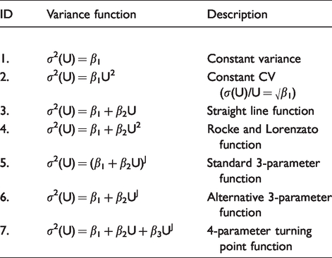
Each of the functions in Table 1 has been used with success in the peer-reviewed literature, but negative mean values create immediate complications. The 4-parameter and alternative 3-parameter functions cannot be estimated because U^J is undefined for negative U unless J is an integer. The Rocke and Lorenzato function fails in the sense that it produces mirror-images around U = 0 and therefore the possibility of negative predicted variances over part of range (the estimation method guarantees positive predicted variances at all data points but not necessarily between them when the function has a turning point; see Figure 1). The constant CV function has no relevance near the detection limit, but fails in any case by predicting σ ² (U) = 0 at U = 0. It also produces mirror images around U = 0. However, the straight line and standard 3-parameter functions can both be estimated in the presence of negative mean values and they both retain the important property of monotonicity, i.e. everywhere increasing, or everywhere decreasing, or constant, thus guaranteeing positive predicted variances across the entire range. In practice, the straight line function is inadequate unless the data have a very short range, leaving the standard 3-parameter function as the sole completely reliable and realistic option from those shown in Table 1. The unavailability of the 4-parameter and alternative 3-parameter functions, and possibly the Rocke and Lorenzato function, represents a potentially serious limitation. Suggested workarounds are outlined in the following sections.

Figure 1.

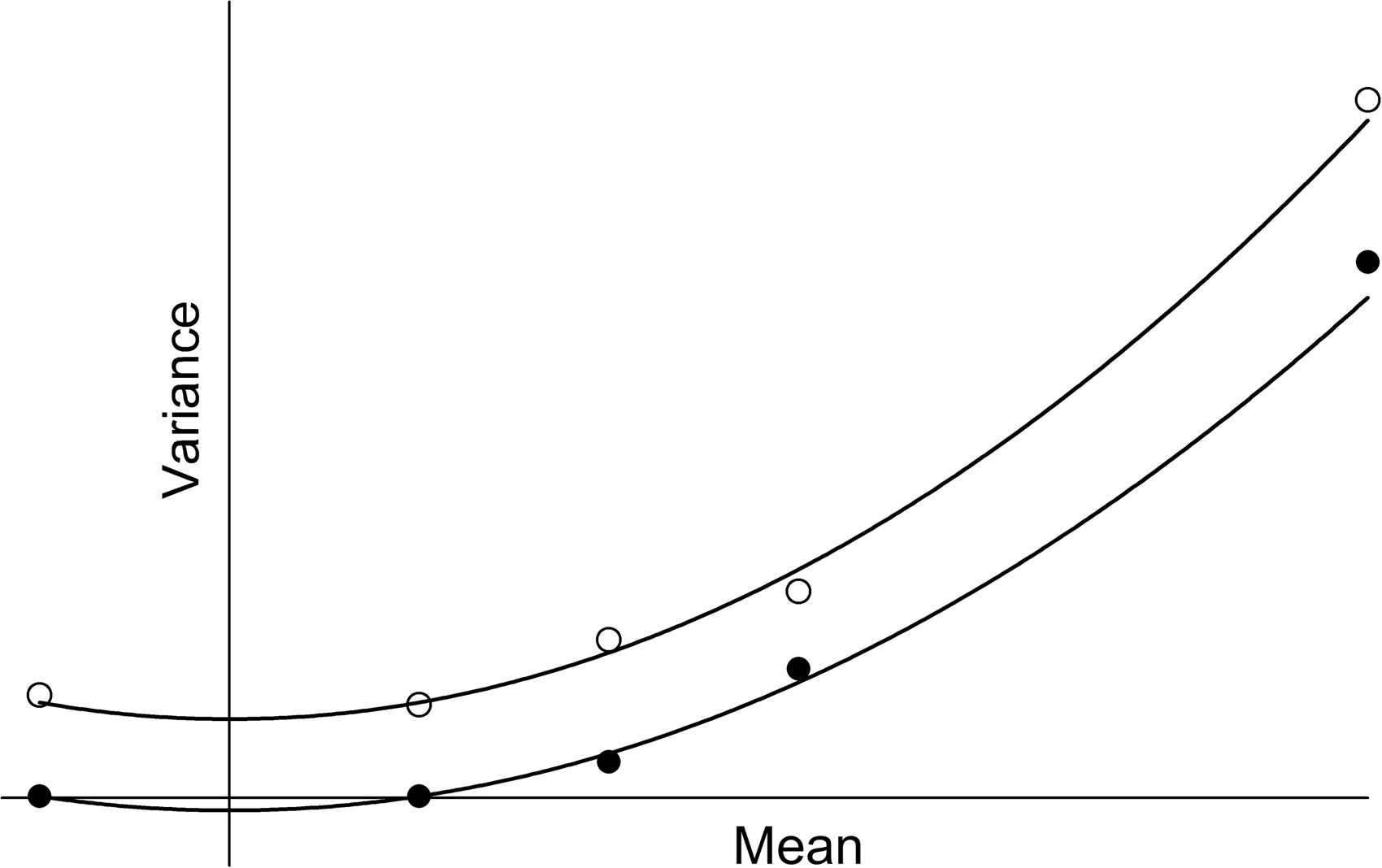
Fit of the Rocke and Lorenzato function, σ ² (U) = β₁ + β₂U ² , to two sets of artificial data (solid and open circles), each of which has one data point with mean < 0. Predicted variance is guaranteed to be positive at all data points and the function is always monotone when all U > 0. However, mirror imaging around U = 0 guarantees a turning point at U = 0 and therefore the possibility of negative predicted variances over part of the range.

Calculation adjustments

Imprecision profiles

Using a variance function to directly estimate imprecision profiles has a long history^17,18 and needs no further comment. When negative mean values are present a case could be made for either of two approaches; include the negative mean values and settle for limited variance function availability, or exclude them and retain access to all available functions (arguably essential in rare cases of a low-end variance turning point). There are additional considerations. Uncertainty plots are most easily interpreted when expressed in terms of CV versus concentration (i.e. precision/imprecision profiles) and such plots necessarily have a lower boundary at U > 0 to avoid infinities. Also, CV plots are usually confined to an upper CV limit of 40–50% to ensure satisfactory readability and the associated concentration values are therefore located a few SDs from zero. In short, imprecision profiles have a natural lower boundary at U > 0 and, quite apart from the function availability issue, it seems reasonable to restrict the data to those with mean values > 0.

LoB and LoD

Armed with an estimate of LoB (by whatever method), the variance function can be used to estimate LoD.^19,20 The advantage of this approach is that the variance function can estimate and thereby accommodate changing uncertainty in the region adjacent to LoB. Normally the variance function data will consist of replications with mean values > LoB and calculations should present no complications. However, if uncensored blank specimen replicates are available, there exists the possibility to either independently estimate LoB from the blanks data, or to include the blank specimen(s) in variance function estimation then calculate LoB using predicted variance at the overall blank specimen mean value. The latter represents a ‘smoothed’ estimate as opposed to a point estimate. The crucial point is that the magnitudes of negative mean values can be expected to be miniscule in relation to the overall range and a simple workaround is to shift all mean values up by a suitable constant prior to analysis, such that the smallest mean value is > 0 (by an arbitrarily small amount). This gives access to all available variance functions and it is a simple matter to back-shift the estimates of LoB, LoD and their confidence intervals. ²⁰

Bland–Altman analysis

Traditional Bland–Altman analysis ² assumes that pair differences exhibit homogeneous scatter when plotted against pair means or, alternatively, that any increase in scatter is proportional to the mean so that homogeneous scatter can be achieved by dividing differences by means ²¹ or by using log transformed data. ² Unfortunately, many data sets do not conform to either of those assumptions and especially when a high density of data is located near the detection limit. A variance function relating variances of pair differences to pair means has the potential to normalize data scatter in these cases thereby extending Bland–Altman analysis to encompass a wider array of data.^22–24 However, when a high density of data is located near the detection limit (i.e. a significant fraction of paired results have been contaminated by left-censoring) and the methods have differing uncertainties (likely to be the rule rather than the exception), then the outcome is spurious bias. ⁴ Bias is particularly pronounced with data left-censored to LoD (or higher) but is also statistically significant with left-censoring to zero.

Uncensored data can be expected to produce instances of negative pair means. Assuming, as per the previous section, that the magnitudes of negative pair means are small in relation to the overall range, it is simple matter to shift the data such that all pair means are > 0, estimate a suitable normalizing variance function (all shown in Table 1 are available), then apply Bland–Altman analysis to the shifted data. Back-shifting the data and Bland–Altman bias and limits of agreement values produces two minor plotting complications. When a log scale is used on the X-axis, or when Bland–Altman results are expressed as percentages, the data and results are necessarily confined to the region where pair means are > 0. The smallest positive pair mean is the natural lower boundary and data points with zero or negative pair means have to be omitted from the plot. Other plotting configurations are not affected.

Regression analysis

The combination of data censoring and unequal uncertainties also result in biased regression parameters. ⁴ Assuming access to uncensored data, there is no problem submitting negative X, Y values for regression analysis. The potential complication lies with estimating variance functions to act as weighting functions (weighting factor = reciprocal of predicted variance). X, Y data shifts cannot be used in this case because back-transformation of the regression parameters and their confidence intervals or joint confidence region is problematic at best and possibly intractable. Variance (weighting) functions should represent day-to-day uncertainty of the X and Y variates because the paired clinical specimen results should ideally be collected across multiple days. Two distinct approaches could be used. First, collect duplicate measurements from each specimen, on different days and in each assay, then estimate X, Y variance functions from the duplicates. Variance function availability is restricted if negative mean values occur for any X or Y duplicate and there is also the likelihood that a relatively small data sample may not yield reliable variance functions (e.g. 50–100 X, Y pairs would imply X and Y variance functions based on just 50–100 duplicates). Second, make use of internal QC or day-to-day method evaluation results. Data sets of this type are usually large and there are no variance function restrictions, but this approach does have the potential drawback that the X, Y concentration range covered by QC or evaluation specimens invariably falls inside the range of the paired results submitted for regression analysis. In other words, using the resulting variance functions as weighting functions is virtually guaranteed to involve some degree of extrapolation outside the concentration range of the data used to estimate the functions. However, a high density of clinical data located near the detection limit presumably implies one or more QC or evaluation specimens located in that region and it is probably reasonable to simply extrapolate the variance function to zero and to use predicted variance at zero to assign weights to negative X or Y values. Extrapolation distances at the low end of the range should be miniscule in well-designed internal QC or method evaluations, and certainly considerably smaller than corresponding distances at the upper end. While ‘exactness’ in the assignment of weights is always the aim, it is necessary in practice to settle for some level of approximation.

Software

Variance function computer programs based on various adaptions of likelihood estimation occurred initially in the immunoassay environment.^25–27 The aim was reliable estimation of the response-error relationship for use as a weighting function in least-squares fitting of the standard curve. The relationship is also an integral part of Ekins’ precision profile method.^9,10 These early programs assumed mean values > 0 because that reflected the reality of the data (assay response measurements). Extending variance function estimation to summarize the uncertainty of test results was a natural progression but adjustments are required to accommodate negative mean values. Variance function program ¹⁴ suppresses estimation in the presence of negative mean values but instead automates the data shifts, back-shifts and extrapolations described in previous sections. Analyse-it ¹⁵ goes a step further and does allow estimation with negative mean values, although restricted in these cases to the subset of variance functions for which estimation is possible. This has potential application if regression weighting function data do extend into the negative region. Importantly, it also gives users the opportunity to simply experiment. Ongoing software developments will doubtless occur.

Summary

There are numerous medical laboratory tests for which the foregoing has no relevance whatsoever because clinical results are well removed from zero. Serum sodium and other electrolytes are obvious examples. However, there are also numerous tests where a high density of clinical results are located in the vicinity of the detection limit and reliable estimation of low-end performance has high importance. In these cases, censored results, and especially those censored to values > 0, can produce seriously misleading statistical summaries (particularly methods comparisons). The requirement for those tasked with evaluating and monitoring test performance is simply the option to access raw uncensored results (including negative results) if and when required. Augmenting regular test output with a parallel stream of raw results, on request, should be trivial given the power and sophistication of modern computing. The main obstacle is not technical but overcoming a decades-long mindset.