Using the variance function to estimate limit of blank,limit of detection and their confidence intervals

Abstract

Background

Implementing International Organization for Standardization definitions of limit of blank and limit of detection requires precision estimates from specimens devoid of analyte (blank specimens) and also from specimens located close to zero. Calculations are straightforward if errors are constant over the relevant concentration range but estimation of the relationship between variability and concentration (variance function) is necessary in the general case when errors are not constant. This study investigated the efficacy of incorporating the variance function into estimation of limit of blank, limit of detection and their confidence intervals.

Methods

Simulated data, designed to encompass the range of properties that would typically be observed in practice, consisted of four distinct relationships between variance and concentration, in combination with large and small variances and three concentration ranges. Four methods of estimating limit of blank were evaluated together with the accuracy of variance function derived estimates of limit of detection and the accuracy of symmetrical 95% confidence intervals constructed from limit of blank and limit of detection constituent variables.

Results

Most limit of blank estimates and all limit of detection estimates showed systematic negative bias but, provided the data concentration range is not too small, the biases were consistently <1% with confidence interval coverages ranging from 92% to 95%. Estimating limit of blank by extrapolating the variance function to zero lost little in comparison with methods based on blank specimen data.

Conclusions

The variance function provides a convenient and reliable way of analyzing data from experiments evaluating detection capability and, provided certain assumptions are tenable, of estimating limit of blank and limit of detection as part of routine internal quality control.

Introduction

Many different definitions and experimental procedures have been proposed for estimating the detection capability of analytical methods. Jiménez-Chacón and Alavrez-Prieto ¹ gave a useful summary of the plethora of different approaches over the last 40 years. More recently it appears that definitions and guidelines published by the International Organization for Standardization (ISO) ² are becoming increasingly widely used. Figure 1 illustrates the concepts. Limit of blank (LoB) is defined as

$\text{LoB}=U0+k1\text{SD}0$

(1) where U₀ is the mean concentration from replicated measurements on a specimen devoid of analyte (blank specimen), SD₀ is the observed SD and k₁ is a coverage factor selected such that it excludes a specified fraction (α) of the density function. Limit of detection (LoD) is defined as

$\text{LoD}=\text{LoB}+k2\text{SD}\text{D}$

(2) where SD_D is the SD at LoD and k₂ is a coverage factor selected such that a specified fraction (β) of the density function centred on LoD lies below LoB. Factors k₁ and k₂ will usually be the same but are not necessarily so, and are typically chosen so that α = β = 0.05. The α region represents false positives (‘detecting’ analyte that is not present) and the β region represents false negatives (failing to detect analyte that is present). LoD is the minimum concentration at which at least 100 × (1 − β)% of observed results can be declared significantly greater than LoB.

Figure 1.

Gaussian distributions illustrating the quantities LoB and LoD where U₀ is the observed mean of replicated blank specimen measurements.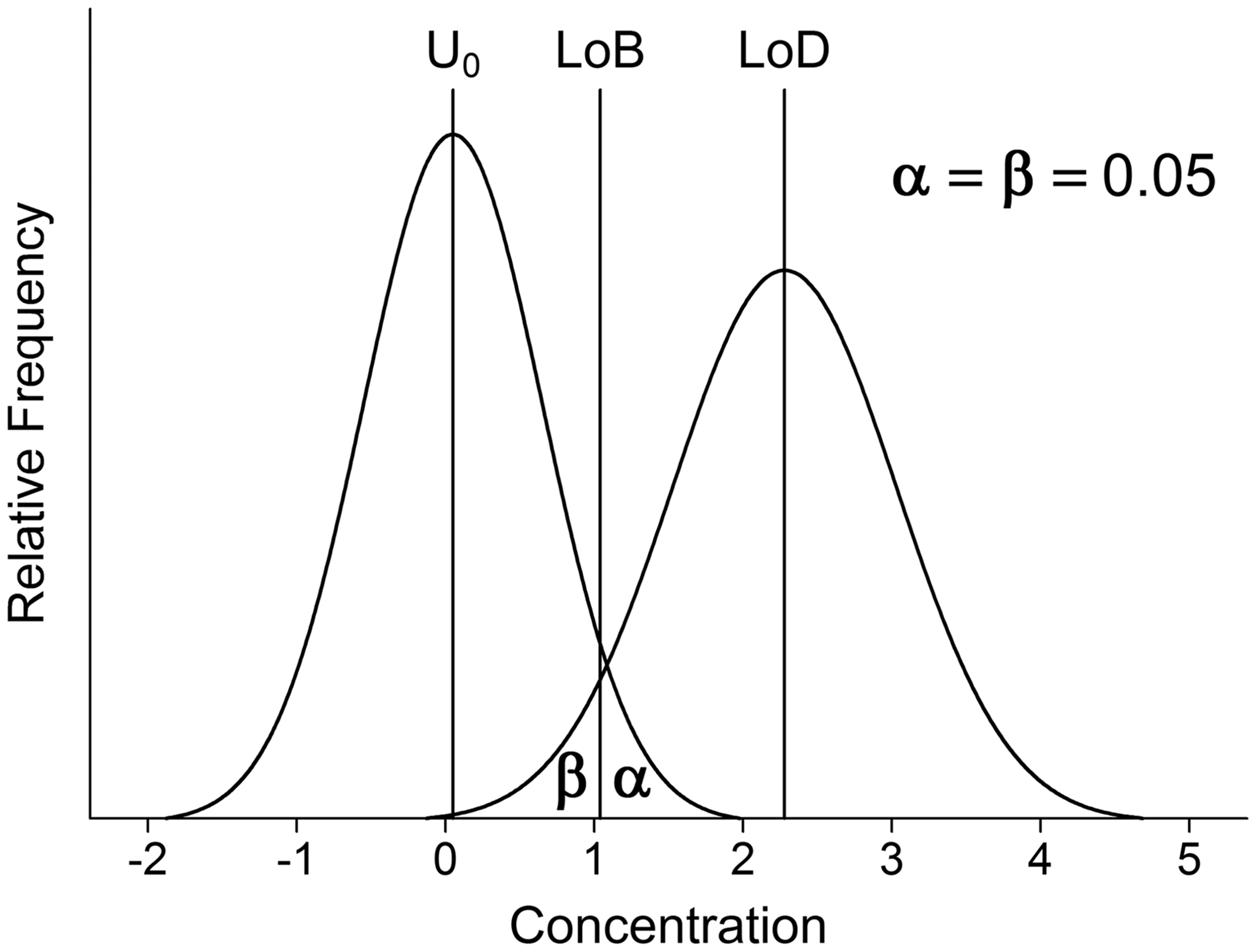

The concept is straightforward but there are practical complications. For example, it is widely assumed that the relevant density functions are Gaussian and therefore factors k₁ and k₂ are 1.645 (subject to adjustment if the number of replicated measurements is relatively small). This assumption is probably reasonable at concentrations around LoD and above. It might also be tenable for blank specimens but unfortunately U₀ and SD₀ cannot be calculated if negative results are truncated to zero and data-reduction output fails to include both raw response (signal) measurements and calibration details. This is a particular problem for immunoassays where manufacturers typically use ‘black box’ principles when designing output from automated instruments. Data rounding is a further potential complication. Moreover, logistic functions are commonly used to model immunoassay calibration relationships and since they are undefined for response measurements on the negative side of the fitted zero response it has to be assumed that a negative-side response deviation equates to a negative result which is the mirror image of the corresponding positive-side deviation. In practice, the routine availability of a complete spectrum of blank specimen results, expressed to a reasonable number of significant figures, is likely to be confined to specialist laboratories able to configure their data-reduction software appropriately, or to those able to acquire the necessary data via a suitable arrangement with a manufacturer. Linnet and Kondratovich ³ proposed the practical solution of estimating LoB nonparametrically as the upper 95th percentile of the distribution of blank specimen results and provided informative worked examples.

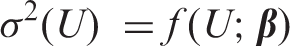
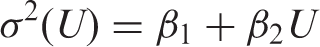
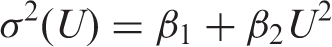
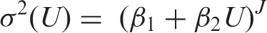
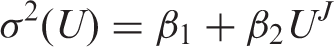
If SD is constant in the vicinity of LoD then SD_D is easily estimated from replicated measurements on one or more suitable specimens and equation (2) yields an immediate estimate of LoD. However, analysis of large databases (e.g. the data described in Sadler ⁴ ) and published data such as in Jiménez-Chacón and Alvarez-Prieto ¹ indicates that errors are not, in general, constant in the vicinity of LoD. If the functional relationship between variance (σ²(U)) and concentration (U) is expressed as

$\sigma 2(U)=f(U;\beta )$

then, from equation (2), LoD is given by the concentration, U, that satisfies

$U=\text{LoB}+k2f(U;\beta )1/2$

or

$U-\text{LoB}-k2f(U;\beta )1/2=0$

(3)

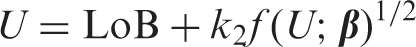
Armed with an estimate of LoB (by whatever method), equation (3) is a general equation for calculating LoD, including the constant SD case where f(U; β )^½ represents a horizontal straight line. After solving, SD_D is the value predicted by the variance function at LoD. However, with the exception of a few cases where f(U; β )^½ has a simple form, equation (3) cannot be reorganized to yield an explicit value of U. It requires iterative solution. The bisection method is perfectly adequate and simple to use. Jiménez-Chacón and Alavrez-Prieto ¹ successfully applied equation (3) to data from flame atomic absorption spectrometry assays for metals using f(U; β ) = (β₁ + β₂U)² and f(U; β ) = β₁ + β₂U² as the variance functions, where β₁ and β₂ are the parameters. The former has the direct solution [U ( = LoD) = (LoB + k₂β₁)/(1 − k₂β₂)]; the latter requires an iterative process.

Equations (1) and (2) indicate that LoB and LoD are just alternative, more informative ways of summarizing precision characteristics at low concentrations. Using the variance function, as per equation (3), not only provides for non-constant errors near zero concentration but also has the potential to routinely incorporate LoD calculations into a single wide-range precision evaluation. It should also be feasible to incorporate the confidence interval (CI) estimated for the variance function ⁵ into CIs for LoB and LoD. In this study simulated data were used to evaluate four methods of estimating LoB, in combination with four variance functions, large and small variances and narrow, moderate and wide range data, with the aim of comparing accuracy of recovered LoB and LoD estimates, accuracy of 95% CIs and relative efficiencies.

Methods

Variance relationships and simulation data

Figure 2 illustrates the target variance relationships which are loosely based on internal QC data from an immunoluminometric assay for serum thyrotropin (TSH). There are two groupings intended to roughly represent the upper and lower limits of what might typically be observed in practice (large and small variances) and within each there are four variance relationships defined by

$\sigma 2(U)=\beta 1+\beta 2U$

(4)

$\sigma 2(U)=\beta 1+\beta 2U2$

(5)

$\sigma 2(U)=(\beta 1+\beta 2U)J$

(6)

$\sigma 2(U)=\beta 1+\beta 2UJ$

(7) where β₁, β₂ and J are the parameters. Equation (5)^1,6,7 is widely used in analytical chemistry while equations (6) ⁸ and (7) ⁹ are specifically aimed at immunoassay data. Three data ranges were defined; narrow (0–0.2 concentration units, as per the inset of Figure 2), moderate (0–10 units) and wide (0–60 units). The narrow range represents a likely range for a targeted LoD experiment, while the moderate and wide ranges are plausible ranges for internal QC specimens or for a general precision experiment. Equation (4) was restricted to the narrow data range, equations (5) to (7) were used over all three ranges to produce 10 (variance function × range) combinations. Four target concentrations (representing specimens) were specified to cover each range. See online supplementary file for details of the variance function parameters and target concentrations.

Figure 2.

Target relationships, plotted as CV versus concentration, represented by four variance functions and two groups representing large and small variances. Labels 1 to 4 denote equations (4) to (7). The inset shows the relationships plotted as SD versus concentration and illustrates the narrow data range used in the simulations.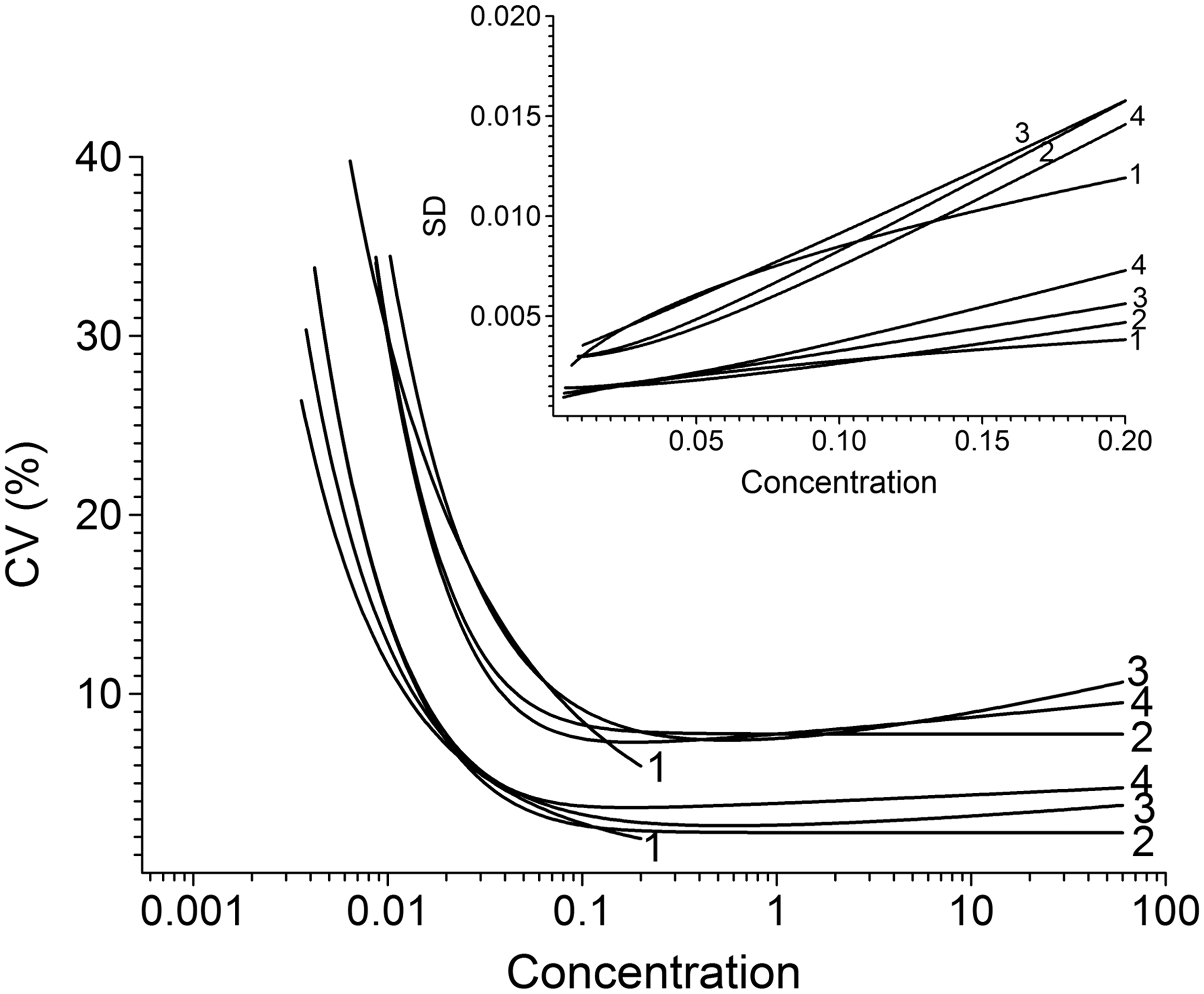

A single simulation data-set consisted firstly of 40 replicate values at each of the four target concentrations, randomly drawn from a Gaussian distribution with mean given by the target concentration and variance predicted by the particular variance function at that concentration. In addition, 40 blank specimen replicates (or 60 replicates in one particular case – see below) were randomly drawn from a Gaussian distribution with mean zero and variance predicted by extrapolating the relevant variance function back to zero (i.e. setting U = 0 in each of equations (4) to (7)).

LoB estimation

Four methods of estimating LoB were evaluated.

A: Predicted

Include all five specimens in variance function estimation. Evaluate equation (1) using, U ₀

mean of the blank specimen replicates.

k ₁

1.645.

SD₀

square root of predicted variance at U₀.

B: Sample

Exclude blank specimen from variance function estimation but assume a Gaussian distribution, i.e. the blank specimen is treated as independent. Evaluate equation (1) using, U ₀

mean of the blank specimen replicates.

k ₁

1.645/C.

SD₀

SD calculated from the blank specimen replicates.

A sample SD underestimates the true underlying SD and C = 1 − 1/[4 × (N − 1)] corrects for the discrepancy where N is the number of replicates. Here N = 40, C = 0.9936 and could possibly be omitted.

C: Nonparametric

Exclude blank specimen from variance function estimation. Assume blank specimen replicates have a non-Gaussian distribution or are not complete, e.g. negative values have been truncated to zero. Compute LoB (α = 0.05) as the value of the (0.95N + 0.5) ordered replicate value, ¹⁰ extrapolating between neighbouring replicates if (0.95N + 0.5) is not an integer. Preliminary simulations showed that the rank values that supposedly represent 95% CIs produced only 83% coverage of the true underlying LoB with N = 40, rising to 89% with N = 50. Therefore, specifically for nonparametric estimation of LoB, the number of blank specimen replicates was increased from 40 to 60. Since (0.95 × 60 + 0.5) = 57.5, LoB is given by the average of the 57th and 58th ordered replicate values. As per Table 1 in Linnet and Kondratovich, ³ the 95% CI is defined by the 54th and 60th ordered replicate values.

D: Extrapolation

Exclude blank specimen entirely. Assume that the variance function estimated from the four higher concentration specimens can be legitimately extrapolated to zero. Evaluate equation (1) using, U ₀

0.

k ₁

1.645.

SD₀

square root of predicted variance at 0.

95% confidence intervals

LoB and LoD are composed of various estimates or approximations of U₀, various estimates of SD₀ and values of SD_D predicted from a variance function. Formulae for combining the errors of these individual constituents into CIs for LoB and LoD are given in the online supplementary file.

Simulations

For each of the 80 data combinations,

$10[\text{variancefunction}\times \text{range}]\times 2[\text{variancesize}]\mathrm{\hspace{1em}\hspace{1em}\hspace{1em}}\times 4[\text{LoBestimationmethod}],$

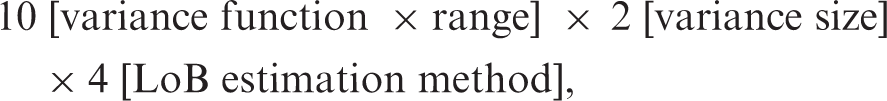
a total of 10,000 sets of simulated data were generated. Variance functions were estimated by conditional likelihood ¹¹ using the automated calculations module of Variance Function Program. ¹² Where estimation was successful (see below), LoB, LoD, and their CIs were saved for analysis.

Limitations

The target variance functions in Figure 2 naturally predict positive variances over the entire range, and also when extrapolated to zero. That does not necessarily extend to variance functions estimated from samples of data. The variance function estimation method ¹¹ guarantees positive predicted variances at all data points but not necessarily outside the range of the data points. LoB method A should always succeed because the blank specimen is included in the estimation process. However, method D (extrapolation) obviously fails if predicted variance ≤ 0 at zero concentration. Less obviously, equation (3) requires predicted variance > 0 at LoB, i.e. after estimating LoB by methods B or C, subsequent calculations to obtain LoD will invariably fail if predicted variance ≤ 0 at LoB. See the online supplementary file for more information.

Results

A detailed tabulation of results is given in the online supplementary file. The main points are illustrated graphically below.

Bias

Each combination of variance function and variance size (Figure 2) produces an exact expected value for LoB and LoD. Figure 3 illustrates the mean values recovered from the 80 simulation experiments expressed as a percentage difference from the target value. A calculation failure rate of 0.12% occurred (970/800,000 sets) consisting of negative predicted variance at zero concentration (582 cases) which negated an LoB estimate by extrapolation (method D), and negative predicted variance at LoB which prevented an estimate of LoD for methods B (190 cases) and C (198 cases). However, failures were entirely confined to the narrow range data. More than 90% (895/970) occurred with the large variance data and more than 75% (734/970) with the use of equation (6).

Figure 3.

Differences between LoB and LoD estimates recovered from simulations and underlying target values, expressed as percentage. Most data points are the mean value from 10,000 sets of simulated data. A few are based on slightly fewer sets (total estimation failures across a row of data points are shown in square brackets). Results are categorized firstly by LoB estimation method; A (predicted), B (sample), C (nonparametric) and D (extrapolation) and secondly by data range; N (narrow), M (moderate) and W (wide). Each row of data points represents either equations (4) to (7) (narrow range) or equations (5) to (7) (moderate and wide ranges) in combination with large variance data (open circles) and small variance data (smaller solid circles).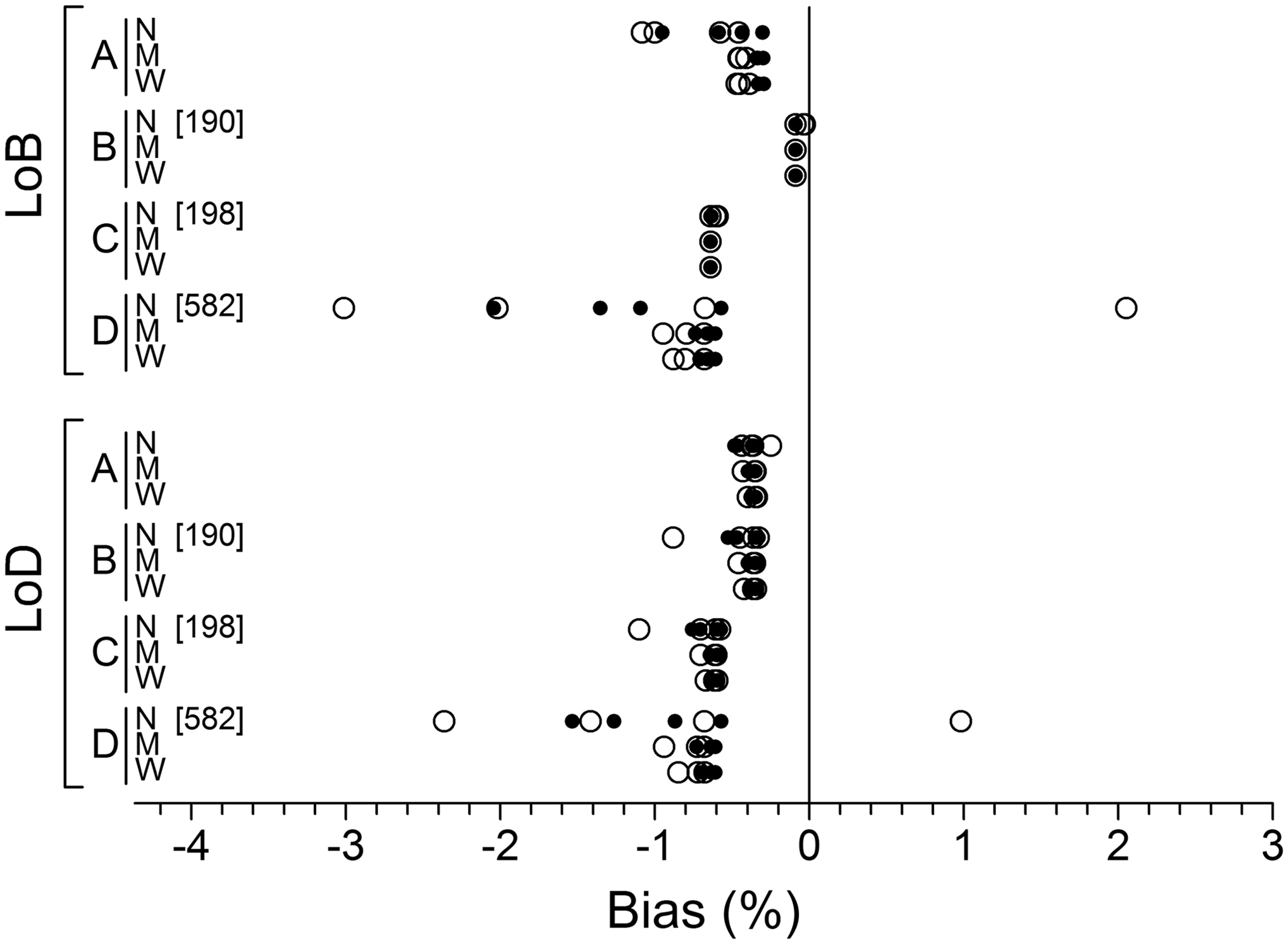

As expected, LoB values estimated from blank specimen means and variances (method B) were not significantly different from target values (P > 0.5 throughout) but all other estimates of LoB and LoD did differ significantly from target values (P < 0.02 throughout). However, ignoring the narrow range data, all results were within 1% of target values and it is worth noting that there appears little difference between estimates obtained from nonparametric analysis of 60 blank specimen replicates (method C) and those relying on extrapolation of the variance function to zero (i.e. complete absence of blank specimen data; method D).

95% confidence intervals

Figure 4 illustrates the percentage of ostensibly 95% CIs that enclosed the true underlying LoB or LoD values. As in the previous section, the largest inaccuracies occurred with narrow range data. Ignoring that range, the least accurate LoB CI coverage occurred with nonparametric analysis (method C), despite the availability of 60 blank specimen replicates. Ignoring the narrow range, the patterns of LoD CI results were remarkable similar, presumably because estimates of SD_D and its error were derived from a common series of variance functions.

Figure 4.

Frequencies of simulation LoB and LoD CIs enclosing the underlying target LoB and LoD values, expressed as percentage. Most data points represent the enclosure rate from 10,000 sets of simulated data. A few are based on slightly fewer sets (total estimation failures across a row of data points are shown in square brackets). See Figure 3 caption for further explanation.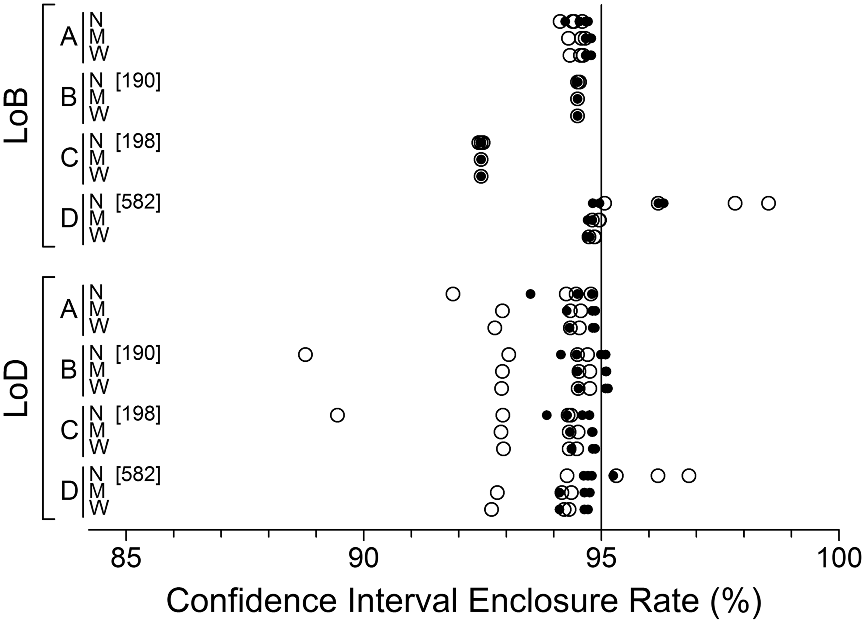

Efficiency

The SD of the LoB and LoD estimates was calculated for each of the 80 simulation combinations and since these SDs vary with mean values, the results were standardized by expressing as a CV, i.e. 100 × observed SD/observed mean. Results are shown in Figure 5. Ignoring the narrow range results, it appears that extrapolating the variance function to zero (method D) loses little in terms of efficiency relative to the methods based on actual blank specimen data.

Figure 5.

Uncertainties of the simulation LoB and LoD estimates expressed as 100 × SD/mean. Most data points are based on 10,000 sets of simulated data. A few are based on slightly fewer sets (total estimation failures across a row of data points are shown in square brackets). See Figure 3 caption for further explanation.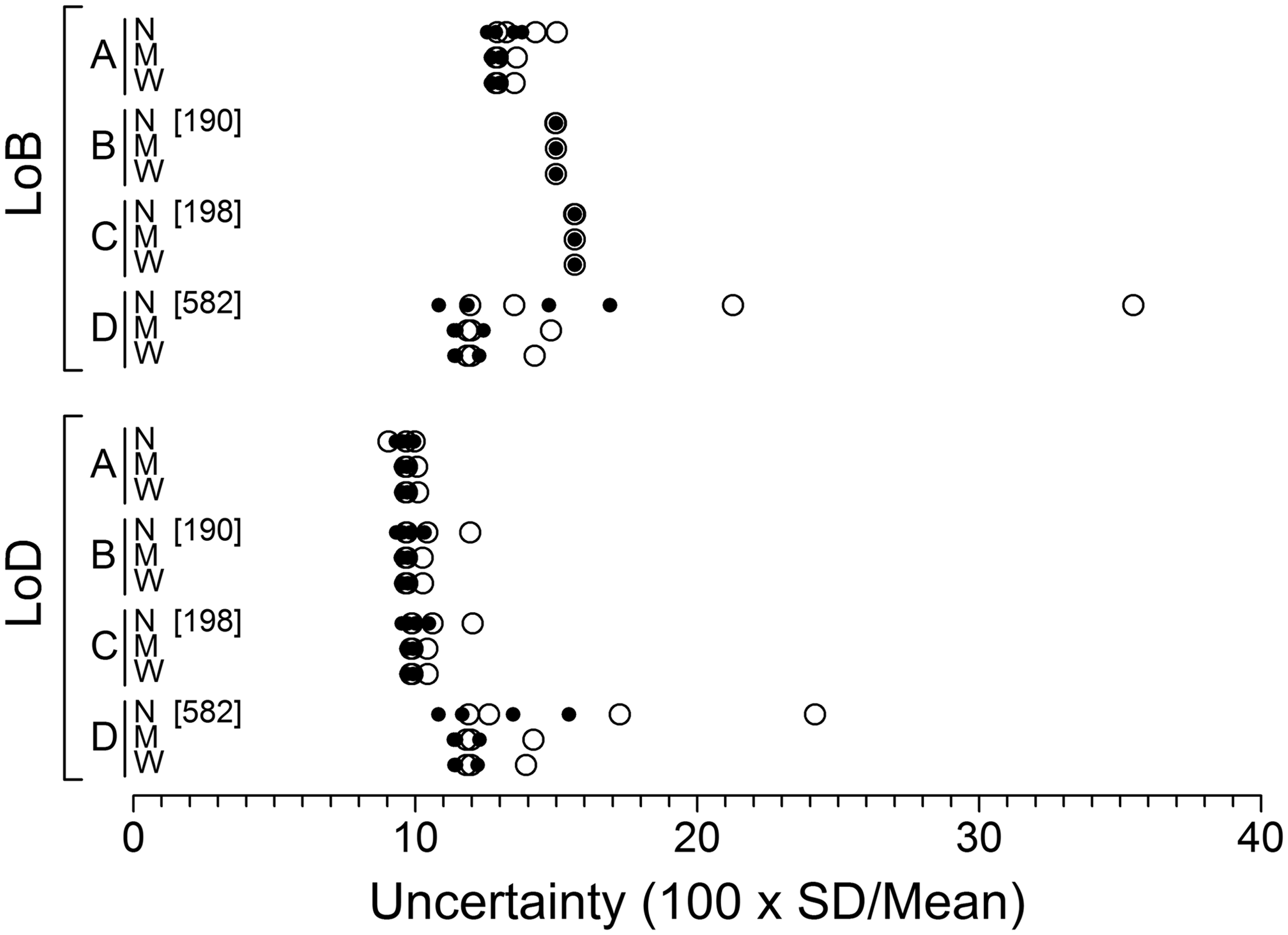

Discussion

The data generated in this study were uncontaminated samples from Gaussian distributions (i.e. no outliers or other aberrant values) and therefore might have been expected to yield unbiased estimates of LoB and LoD and perfectly accurate CIs. However, simulation run sizes of 10,000 have considerable statistical power and clearly demonstrate that the variance function methods used here resulted in systematic negative bias in the estimates of both LoB and LoD. This, in turn, was probably a factor in CIs systematically failing to achieve the expected 95% enclosure of true underlying values. Nevertheless, the biases and inaccuracies are relatively small and the estimates illustrated in Figures 3 and 4 could be regarded, for practical purposes, as useable approximations.

There was a clear range related effect. Estimation failures and the largest biases and inaccuracies occurred exclusively with narrow range data. This contradicts the intuitive notion that packing as much data as possible into the immediate vicinity of LoD will ‘obviously’ yield improved estimates. That would certainly be true if variance was constant in the vicinity of LoD, but when variance changes with concentration the crucial factor is the reliability of estimation of the underlying relationship, i.e. f(U; β ) in equation (3). In general, the wider the range of values for the independent variable the smaller the uncertainty associated with the estimated variance function. However, an underlying variance function factor should be noted. Equation (6) possesses considerable latent flexibility, necessary to successfully model wide range immunoassay data, but as previously noted, ⁴ performs poorly (overly flexible) when applied to narrow range samples of data and especially when relative change in variance is small. It accounted for more than 75% of estimation failures and for the majority of the extreme biases and CI inaccuracies. At the other extreme equation (5) was alone in delivering a zero failure rate.

The wide-range relationships illustrated in Figure 2 represent relative concentration changes (maximum:minimum) of up to 16,000-fold and relative changes in variance of up to 4-million fold. The latter is completely disguised when transformed and plotted as CV versus concentration. Contrary to what might be expected, data points with means and variances far removed from LoD do not unduly influence the variance function fit in the vicinity of LoD. The estimation method ¹¹ takes full account of the sampling variability of variances and weights each data point by the factor, (N − 1)/ $({\sigma }_p^2)2$ , where N is the number of replicates and ${\sigma }_p^2$ denotes predicted variance at that data point. See also Finney and Phillips ¹³ and Raab. ¹⁴ Data points near LoD receive enormous weighting relative to those at higher concentrations which ensures that very wide ranges can be used without adverse low-end consequences.

This study investigated the consequences of disregarding blank specimen replicates entirely and estimating SD₀ (hence LoB) by extrapolation (LoB method D). In the case of the narrow range data, illustrated in the inset of Figure 2, extrapolation distances are clearly ‘discernable’ and represent 2–5% of the range. However, this reduces to 0.03–0.1% with the moderate data range and <0.02% with the wide data range (i.e. <1 part in 5000). If a variance relationship appears reliably estimated from data at LoD and higher concentrations, it seems improbable that a significant shift in precision characteristics would occur within the vanishingly small extrapolation distances. However, that factor together with the distribution properties of blank specimen replicates requires assessment on a case-by-case basis. Given that manufacturers typically withhold essential details (especially in the case of immunoassays), it could be argued that they have an obligation to assist clinical laboratories in that regard by routinely publishing blank specimen data alongside the usual precision estimates.

The simulations assumed a Gaussian distribution for blank specimen replicates and mean, variance values that are an exact extrapolation of the functions shown in Figure 2. If tenable with real data, results suggest that extrapolation loses little in comparison with estimates based on data. That is not a total surprise given the miniscule extrapolation distances. It is also worth noting that extrapolation estimates of SD₀ will invariably be based on the precision characteristics of genuine clinical specimens or pools. In contrast, preparation of blank specimens can, in some cases, require chemical or other manipulation and therefore the possibility of precision characteristics that do not mimic those of genuine clinical specimens.

In practice, formal experiments to estimate LoB and LoD usually include two or more blank specimens (i.e. at least some attempt to provide for possible precision differences between specimens) and several specimens in the region of LoD. Gaussian distributions can usually be safely assumed at LoD and higher concentrations. If blank specimen replicates also appear approximately Gaussian then the blank specimen data point(s) could be included in variance function estimation (LoB method A), or treated as independent (LoB method B). The latter appears to have slight advantage in terms of bias (Figure 3). Nonparametric analysis ³ provides fallback (LoB method C). However, experiments of that type (in fact precision experiments in general) are often performed over a short time span and involve a single calibration event and a single lot of all reagents. Resulting estimates are not necessarily a good indicator of clinical laboratory outputs because potentially important error sources have been excluded, e.g. errors associated with multiple lots of calibration materials, multiple re-calibrations, multiple lots of reagents, medium to long term instrument wear and tear, operator differences (manual assays) and possibly effects due to a ‘carefully’ performed experiment versus the pressured conditions of a high workload clinical laboratory. The four specimen, 40 replicate, moderate and wide range designs used here were deliberately chosen to reflect daily internal QC measurements over a two month period. A target QC concentration in the vicinity of LoD was assumed to be typical for assays where detection capability is of high importance. By organizing QC data on a roll-on roll-off basis, and assuming extrapolation has been verified as tenable, the variance function approach has the potential to convert routine data into regularly updated estimates of LoB and LoD. No special or additional measurements are required and such estimates reflect current detection capability under clinical working conditions.

Previous paragraphs stressed extrapolation and the clinical laboratory context, but the variance function approach can be used with any suitable experimental data and any LoB estimation method. The computer program ¹² used to estimate the variance functions has been updated to automate the LoB, LoD and CI calculations described here.