Methods comparison biases due to differing uncertainties and data censoring

Abstract

Background

Measurements on clinical specimens that contain no analyte, or very low amounts of analyte, unavoidably generate assay response (signal) measurements that fall on the ‘negative’ side of the fitted zero response. It is virtually universal practice to left-censor such measurements to zero and this is frequently extended by left-censoring to the assay limit of detection (LoD) value for reporting purposes. This study considers the effect of censoring on methods comparison analysis.

Methods

Paired results were randomly generated from two hypothetical assays with zero bias, firstly assuming equal uncertainty near zero and secondly with uncertainties that differed by a moderate 50% near zero. In both cases results were left-censored to zero and to LoD and further subsets were extracted representing partial and complete removal of censored results. All data sets were subjected to overall bias evaluation and Bland–Altman and Deming regression analyses.

Results

The combination of differing uncertainties and data censoring produced spurious biases by both Bland–Altman and regression analysis, regardless of whether censored results were retained or discarded. Biases were small for data left-censored to zero but were non-trivial with LoD-censoring. Imposing a lower limit aimed at eliminating the influence of censored results did not resolve the problem.

Conclusions

When high proportion of clinical results are located near zero, caution is required when using censored data (and especially LoD-censored data) in methods comparison studies. Optional access to negative results would rectify the problem, but requires the cooperation of manufacturers.

Introduction

Bland–Altman analysis ¹ and Deming regression ² are widely used to evaluate the agreement between two analytical methods. However, issues arise when clinically important results are located near assay detection limits. Meaningful methods comparison in those cases requires accumulation of paired results near zero and the sharp rise in CV in that region means that traditional Bland–Altman analysis invariably produces misleading or even meaningless limits of agreement. That particular problem can be overcome by transforming the data using a variance function estimated from pair differences, as previously described.^3–5

An additional issue is the impact of censored data. It is standard practice, at least for immunoassays, to left-censor apparently negative results to zero and common practice to report results left-censored to limit of detection (LoD) values, or to some similar lower limit.

It is easily recognized that the presence of censored values produces pair differences which systematically underestimate the true underlying differences. It is probably less obvious that simply excluding all such pairs does not resolve the matter. More importantly, it may not be obvious that when methods under comparison have differing uncertainty characteristics near zero (i.e. differing LoD values), spurious bias estimates occur (both Bland–Altman and regression analysis) regardless of whether pairs containing censored values are retained or excluded. A simple simulation experiment is used here to illustrate these effects.

Methods

Equal uncertainty case

The model is a pair of assays with zero bias and identical uncertainty properties. N = 51 equally spaced target mean values covering the interval 0–10 units were pre-set (0, 0.2, 0.4, … , 9.8, 10.0). At each target mean value two Gaussian distributions (arbitrarily designated X, Method B and Y, Method A, respectively) with mean = target mean and SD =1.0 were used to randomly draw 250,000 paired results. Each result was rounded to two decimal places. The data extend to 10 SDs from zero and, by the usual definition, ⁶ LoD is located at 3.29 units (i.e. 1.645 SD + 1.645 SD). Obviously many negative results occurred at the lower end of the target interval.

For each of the 51 groups of 250,000 pairs the following combinations were considered; (a) all data, (b) negative results left-censored to zero and all data retained, (c) as for (b) but exclusion of pairs with both values censored, (d) as for (b) but exclusion of pairs with either value censored. In each case three quantities were calculated; mean of Method A and Method B values, mean of (Method A − Method B) differences (Bland–Altman bias), and the SD of the differences (used to calculate Bland–Altman limits of agreement). The calculations were repeated for combinations (b), (c) and (d) except that results were left-censored to 3.29 (LoD).

Given the very large sample size, combination (a) should yield 51 sets of results which accurately recover true underlying values, i.e. mean of Method A and Method B = target mean, mean (Method A − Method B) difference = 0 and SD of differences = √2. The aim is to evaluate departures from those values caused by data censoring. Data patterns are also of interest. Since it is not feasible to plot 51 ×  250,000 possible data points, the first 1000 pairs from each set of 250,000 were retained for illustrative purposes and for submitting to Bland–Altman and regression analyses (see Supplementary file). These 51 sets of 1000 pairs were subjected to the same censoring combinations as described above.

Differing uncertainty case

The model is a pair of assays with zero bias and differing uncertainties. The data generation described in the previous section was repeated except that the second Gaussian distribution used at each target mean value was assigned SD = 1.5, i.e. measurement SD for the second hypothetical assay (Y, Method A) is 50% greater than the first (X, Method B) and consequently LoD values are 4.935 and 3.29, respectively. The calculations and retention scheme described in the previous section were repeated except that when left-censoring to LoD values the Method A and Method B results were left-censored to 4.935 and 3.29, respectively. The expected SD of pair differences in this case is (1² + 1.5²)^½ or 1.8028.

Results

The main results of the experiments are summarised here. The consequences for Bland–Altman and regression analyses are illustrated in detail in the Supplementary file.

Equal uncertainty

As could have been predicted, no data combination showed evidence of (Method A − Method B) bias, or Deming regression bias, because regardless of whether data are censored to zero or to LoD (or to any other common value), the effects are equivalent for both pair values.

In contrast, Figure 1 illustrates SDs of pair differences plotted against pair mean values. The expected means and SDs were reliably recovered from the uncensored data. The slight jittering simply reflects experimental sampling variation. Censored data show considerable biases both in observed mean values and observed SDs and, as expected, these effects are more marked for data censored to LoD. Note that excluding all pairs that include a censored value did not eliminate SD biases. The impact on Bland–Altman limits of agreement are tabulated in the Supplementary file.

Figure 1.

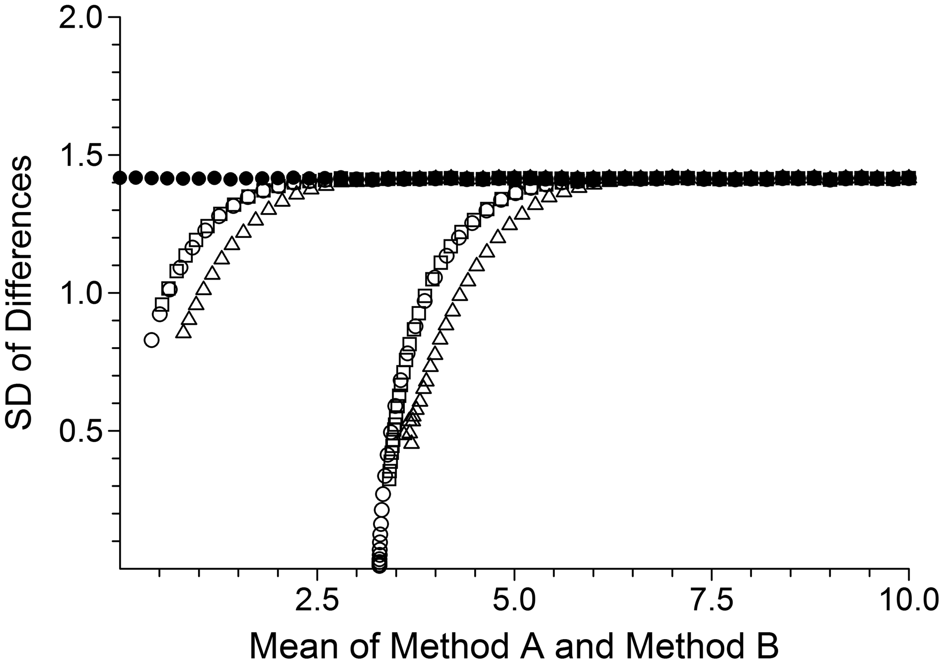
Equal uncertainty case. Solid circles illustrate observed means and SDs for the uncensored data. Open circles, open squares and open triangles illustrate, respectively, corresponding means and SDs after data censoring but all results retained, data censoring and exclusion of all pairs with both values censored, and data censoring and exclusion of all pairs with either value censored. The left and right groupings illustrate left-censoring to zero and to LoD, respectively.

Differing uncertainty

(Method A − Method B) biases were evident for all combinations involving differing uncertainties and censored data. Biases were small for data censored to zero and those results are illustrated in the Supplementary file. The more pronounced biases observed with censoring to LoD are shown in Figure 2. The observed biases are plotted with large symbols over a sample of the randomly drawn pairs (i.e. the 51 × 1000 pairs retained for illustrative purposes). The latter also illustrate how the data would appear in a Bland–Altman plot. Close inspection of Figure 2(a) shows that the underlying pair data have the shape of a forward leaning parallelogram. In general, the greater the difference in the uncertainties the more pronounced the forward lean. Nevertheless, this did not affect the accurate recovery of the target means and differences. A pair of intersecting data ‘boundaries’ is clearly visible for the censored data in Figure 2(b) and these represent pairs where one of the two values had been censored. The intersection point is the location of pairs where both values had been censored (i.e. Mean = (3.29 + 4.935)/2 = 4.11 units and Bias = 4.935 − 3.29 = 1.645 units). The partial and complete exclusion of pairs containing censored values simply removes data points from the intersection point, Figure 2(c), and from the boundaries, Figure 2(d), respectively, but does not alter the underlying data pattern.

Figure 2.

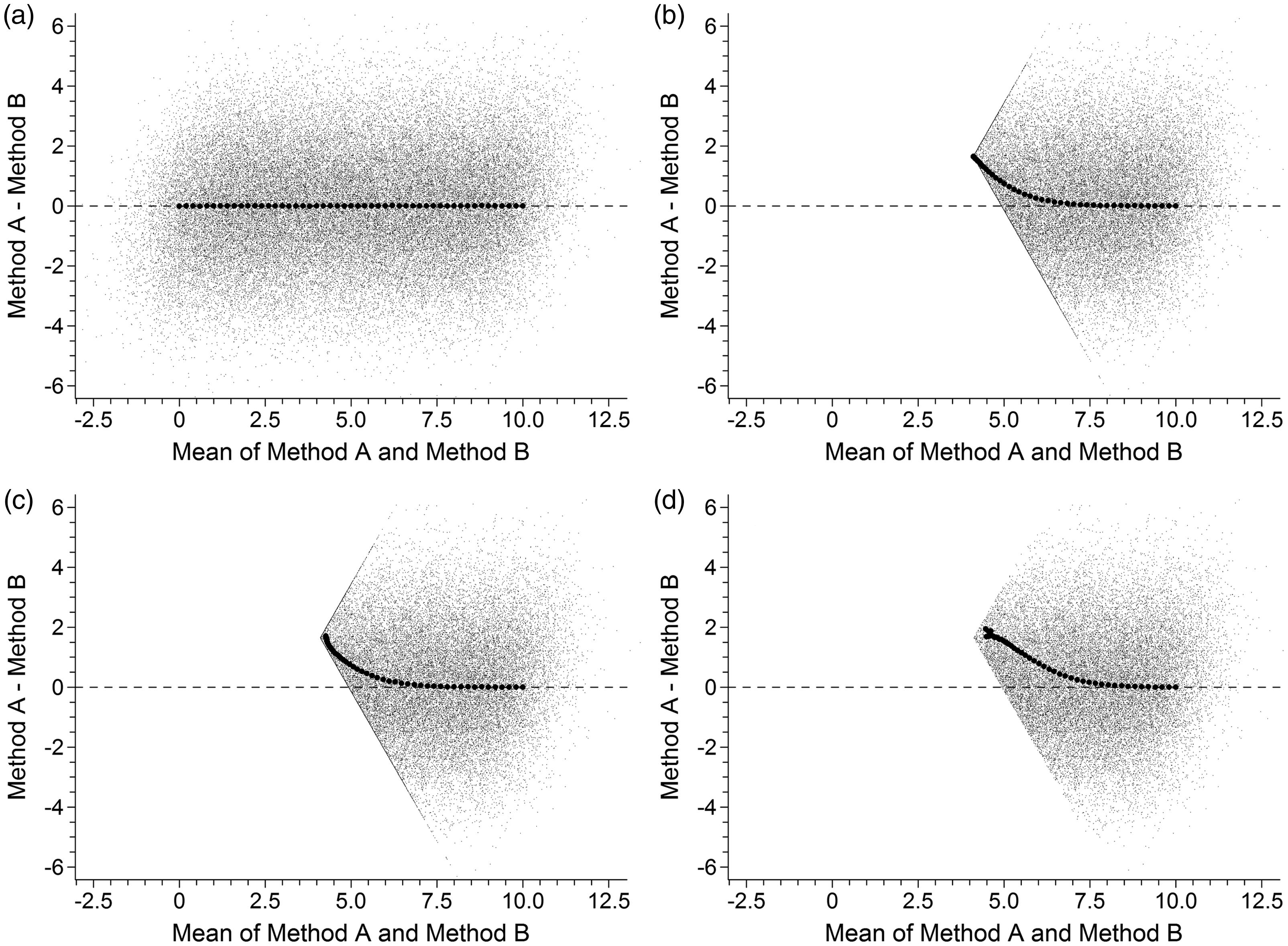
Differing uncertainties and data left-censored to respective LoD values. The larger solid circles illustrate observed pair means and differences averaged within each of the 51 sets of 250,000 pairs. The smaller data points are the subset of 51 × 1000 pairs, retained for illustrative purposes, which indicate how the underlying pair data would appear in a Bland–Altman plot. The four panels represent: (a) uncensored data, (b) censored data and all results retained, (c) censored data with exclusion of pairs with both values censored, and (d) censored data with exclusion of pairs with either value censored.

SDs of pair differences are illustrated in Figure 3 and show virtually identical patterns to those in the equal uncertainty case (Figure 1), but shifted to the right. The data patterns in Figure 2(b) to (d) provide insight into why observed SDs of pair differences show little change following the successive removal of censored data.

Figure 3.

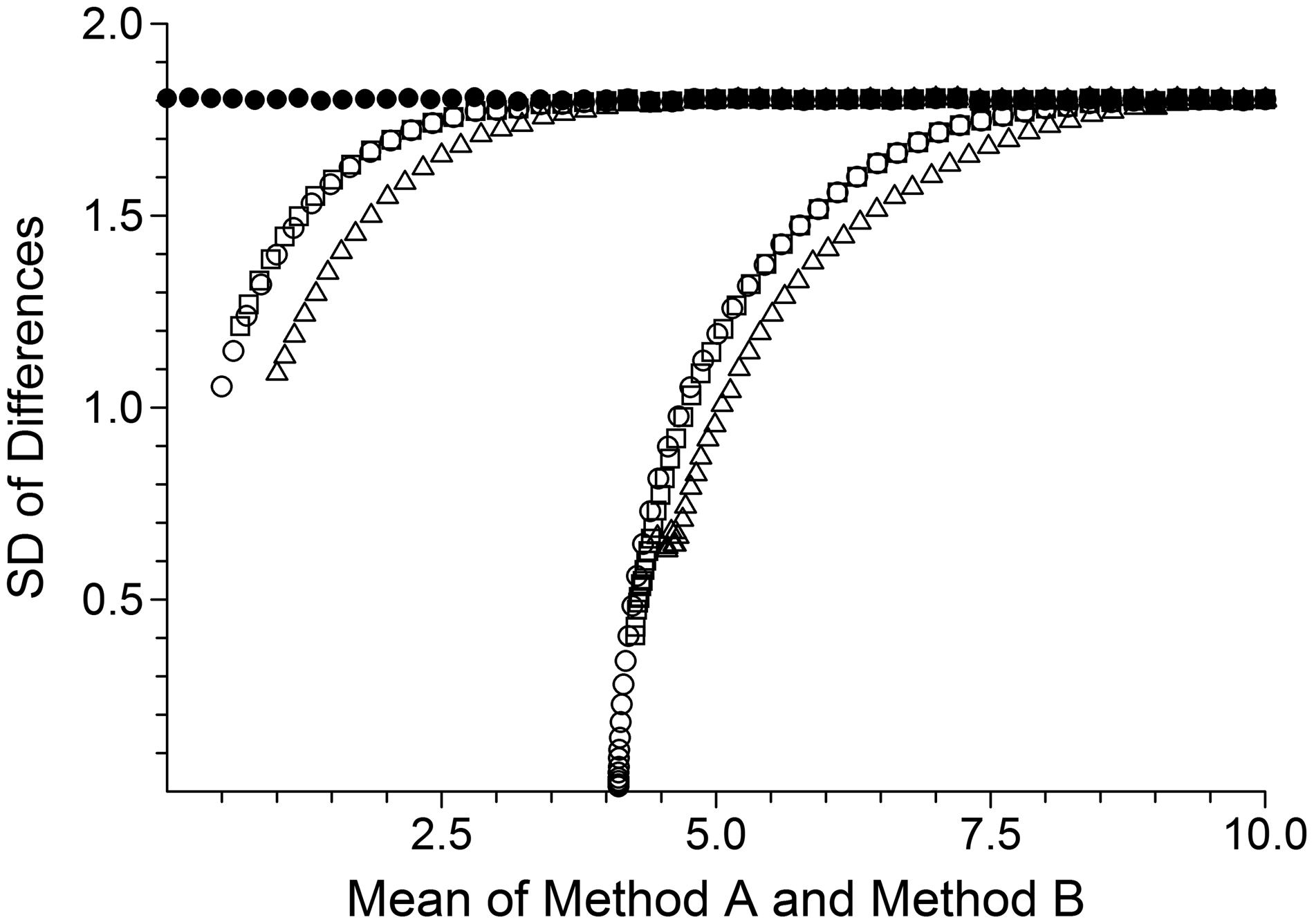
Differing uncertainty case. Solid circles illustrate observed means and SDs for the uncensored data. Open circles, open squares and open triangles illustrate, respectively, corresponding means and SDs after data censoring but all results retained, data censoring and exclusion of all pairs with both values censored, and data censoring and exclusion of all pairs with either value censored. The left and right groupings illustrate left-censoring to zero and to LoD, respectively.

Discussion

The effects illustrated here will of course be ‘diluted’, possibly to insignificance, when a high proportion of paired methods comparison data is well removed from zero. This study addresses the particular issue of methods comparison when a relatively high proportion of pair data is located near zero (although the overall range of mean values might be large). It is clear from the figures that the effects of censoring extend (as expected) to about 2.5 SDs above zero or above LoD, depending on which mode of censoring has been applied, and that should be taken to mean the larger of the SD and LoD values when the methods have differing precision characteristics. When mean values span a wide concentration range, boundaries similar to those illustrated in Figure 2(b) to (d) might not be easily discerned on a Bland–Altman plot with linear X-axis scale, but should be readily apparent on a logarithmic X-axis scale.

Conducting a methods comparison using results censored to LoD is appealing because the data are likely to be readily accessible (e.g. stored in a clinical database) and, moreover, it seems intuitively correct to use them because these are the results that are actually reported out. Unfortunately, in the presence of differing uncertainties, spurious bias, equivalent to the difference in LoD values, occurs at the lower data extreme. The rather moderate 50% difference in LoD values used here might be typical of a point-of-care instrument versus a main laboratory instrument, but larger differences are certainly possible. In the extreme, 10-fold differences are well known with the so called ‘generational’ improvements in immunoassay sensitivities. It is easy to submit such data to Bland–Altman or regression computer programs without appreciating the underlying low-end consequences.

In the case of differing uncertainties, how should a serious methods comparison proceed when a high proportion of data is located near zero? An obvious recommendation is to use only raw results (i.e. typically left-censored to zero) which markedly reduces not only the range of mean values over which spurious effects occur, but also the sizes of the effects. As indicated by the figures, discarding all pairs which include a LoD-censored value might slightly improve bias and Bland–Altman limits of agreement issues but it does not resolve them. Unpalatable though it might be, the graphs suggest that biases could be completely abolished by discarding all pairs whose mean values lie within the region of influence of the censored data. The biases shown in any of Figure 2(b) to (d), for example, suggest a mean value cut-off at around 7.5 units. However, imposing a lower limit failed; a completely unexpected result. The reason is a matter of symmetry. Imposing a lower cut-off on data such as those in Figure 2 sets a vertical lower boundary, but the upper boundary has a systematic diagonal orientation due to unequal uncertainties. That combination equates to asymmetry and manifests as bias, whether evaluated by Bland–Altman analysis or regression analysis. These secondary bias effects are illustrated in the Supplementary file.

The problems discussed here disappear if laboratory analysts were able to access negative results (as per Figure 2(a), for example). Quite apart from eliminating censoring effects, the data symmetry necessary for unbiased estimates would be preserved. Moreover, analyses would have improved efficiency because all available information is utilised. A complication in the case of immunoassays is that the logistic functions commonly used to model standard curves cannot directly produce a result for response measurements that fall on the ‘negative’ side of the fitted zero response (result undefined because the calculation involves the logarithm of a negative number). Nevertheless, there is more than one way to obtain estimates. The simplest is to assume response measurements are symmetrically distributed about their mean values and that variance is constant in the immediate vicinity of zero. A negative result is therefore well approximated by mirroring a negative side response measurement onto the positive side and interpolating as usual. The calculation is trivial, but does require access to raw response measurements, the standard curve model and the parameters of the current standard curve fit. Given the general reluctance of manufacturers to disclose the internal details of their methods it seems logical that manufacturers should perform the calculations. In the vast majority of cases negative results are not needed and would not be of the slightest interest to laboratory analysts, but there is nothing to prevent instrument output being supplemented, on user request, by a parallel stream of results which include negative value calculations. Methods comparison studies would be facilitated if manufacturers made the effort to provide such an option. Is it likely to happen? That is an open question.

Supplemental Material

Supplemental material for Methods comparison biases due to differing uncertainties and data censoring

Supplemental Material for Methods comparison biases due to differing uncertainties and data censoring by William A Sadler in Annals of Clinical Biochemistry