Using the variance function to generalize Bland–Altman analysis

Abstract

Background

Bland–Altman analysis is a popular and widely used method for assessing the level of agreement between two analytical methods. An important assumption is that paired method differences exhibit approximately constant (homogeneous) scatter when plotted against pair means. This allows estimation of limits of agreement which retain validity across the entire range of mean values. In practice, pair differences often increase systematically with the mean and Bland and Altman used log transformed data to achieve approximately homogeneous scatter. Unfortunately, a logarithmic transformation fails when data are located near the detection limit of an assay (a region that is often of considerable clinical importance).

Methods

Simulated thyrotropin data are used to illustrate how a variance function, estimated from pair differences, can be used to transform problematic data into a form suitable for traditional Bland–Altman analysis. Simulated and real data sets are used in a supplementary file to illustrate and offer practical solutions to potential problems.

Results

Following transformation by variance function, Bland–Altman results can be readily interpreted by back-transformation either to the original measurement scale or as percentage values. Limits of agreement are no longer horizontal straight lines, but their shapes simply reflect error characteristics which are (or should be) thoroughly familiar to laboratory analysts.

Conclusions

The method is completely general and in principle requires only the estimation of a variance function that reliably describes the relationship between the variances of pair differences and their mean values. A computer program is available which performs the necessary calculations.

Introduction

Bland–Altman analysis ¹ is so widely used that it hardly needs introduction. In brief, pair differences in a methods comparison are plotted against pair means, and the mean and SD of the differences are calculated. The mean difference is an estimate of bias with confidence interval (CI) ts/√N where t is the critical Student's t value with N–1 degrees-of-freedom, s is the SD of the differences and N is the number of paired results. Assuming the differences have Gaussian distributions, Bland–Altman 95% limits of agreement are given by mean ± 1.96 s with approximate CI, √3ts/√N (derivation given in Bland and Altman ² ). Meaningful agreement limits rely implicitly on a homogeneous scatter of pair differences across the range of mean values. In practice, measurement errors (hence pair differences) often increase markedly over the range. Bland and Altman handled that data pattern by assuming constant CV and using log transformed data to normalize the scatter of the pair differences. An equivalent normalizing strategy, first suggested by Eksborg, ³ is the transformation 100d _i /U _i where d _i and U _i are, respectively, the difference and mean of the ith pair (i = 1, 2, … , N). This transformation has no effect on the X-axis of Bland–Altman plots. In both cases, the mean difference (bias) and limits of agreement can be directly interpreted as percentage values.

Unfortunately, many data-sets do not conform to the simple constant variance or constant CV assumptions of traditional Bland–Altman analysis. In particular, clinically crucial results from numerous immunoassays occur in the vicinity of the assay detection limit where CV rises sharply. Moreover, immunoassays often exhibit a marked upturn in CV at both ends of the measurement range and on rare occasions a variance turning point near the assay detection limit. ⁴ The variance function can provide a solution. The success of the transformation 100d _i /U _i in cases of constant CV is not because of some fortuitous property of the U _i , but because constant CV implies SD directly proportional to U. Therefore, 100d _i /U _i is equivalent to 100d _i /SD _i (or simply d _i /SD _i ) where SD _i is predicted SD of the pair differences evaluated at U _i . In this specific context, 100d _i /U _i is preferred simply because the resulting Bland–Altman quantities have a simple interpretation as percentages. The general normalizing transformation is d _i /f(U)^½, where f(U) is a suitable variance function which describes the relationship between the variance of the d _i and U. Recognizing this, Hawkins^5,6 used the Rocke and Lorenzato function ⁷

$$\text{f}\left(\text{U}\right)={\beta }_{\text{1}}+{\beta }_{\text{2}}{\text{U}}^{\text{2}}$$

(1)

where β₁ and β₂ are parameters to illustrate successful normalization of paired oestradiol results when the traditional logarithmic (or equivalent 100d _i /U _i ) transformation failed at the low end of the range. He also introduced a probably long overdue enhancement by adapting the Breusch-Pagan statistic^8,9 as an objective test of the success (or otherwise) of a normalizing transformation.

The complication, following transformation by d _i /f(U)^½, is interpretation of the bias and limits of agreement values. In practice, it is a simple matter to back-transform them, as Hawkins illustrated, either to the original measurement scale or as percentages. In this study, simulated thyrotropin (TSH) data are used to illustrate the general d _i /f(U)^½ transformation and formulae are derived for back-transforming CIs. A supplementary file contains simulated and real data examples which draw attention to practical issues.

Methods

Simulated methods comparison data

Data from a precision evaluation ¹⁰ of TSH measurement on the ‘Access’ instrument (Beckman Coulter, Fullerton CA, USA) were used to estimate the variance function ¹¹

$$\text{f}\left(\text{U}\right)={\left({\beta }_{\text{1}}+{\beta }_{\text{2}}\text{U}\right)}^{\text{J}}$$

(2)

where U ranged from 0.0156 to 27.19 mU/L and β₁ = 0.008936, β₂ = 0.04401 and J = 2.4718 are the fitted parameters. A typical clinically observed distribution of N = 125 values between 0.0156 and 27.19 was preset (i.e. a relatively high density at the low end of the range) and at each of these values a pair of results were randomly drawn from a Gaussian distribution with variance as predicted by equation (2). The 125 paired results (tabulated in the supplementary file) were submitted as duplicates to estimate a (normalizing) variance function (equation (2)). ¹¹ Bland–Altman analysis was conducted using the raw pair differences (d _i ) and transformed as 100d _i /U _i and as d _i /f(U)^½.

Breusch-Pagan statistic

As adapted by Hawkins, ⁶ the d _i are first scaled to mean value zero. Denoting the scaled values as θ _i , quantities θ _i ²/D are regressed on the U _i , where D is the overall mean of the θ _i ². SS_reg/2, where SS_reg is the sum of squares attributable to regression, is asymptotically distributed as χ² with one degree-of-freedom. Hawkins’ description omitted the initial scaling step, doubtless a simple oversight. Tests based on χ² can lose accuracy at small N and a preliminary check was performed. Sets of N = 1000, N = 150, N = 100 and N = 50 pairs were randomly drawn from Gaussian distributions (uniformly distributed U between 10 and 100 with constant variance 1.0) and in each case subjected to the regression described. The experiment was repeated 500,000 times (10,000 samples × 50 different random number seeds) and overall frequencies of SS_reg/2 values > 3.84146 were determined (the critical 0.05 value for χ² with one degree-of-freedom). Observed frequencies for N = 1000, 150, 100 and 50 were 0.0499, 0.0482, 0.0477 and 0.0455, respectively. Under somewhat idealized conditions, the test retained reasonable accuracy at sample sizes typical of Bland–Altman analyses.

Back-transformation

Following normalization by d _i /f(U)^½, the transformed data points and bias and limits of agreement values can be back-transformed to the original scale by simply multiplying by f(U)^½, evaluated at U _i . Likewise, back-transformed data and summary values can be expressed as percentages using the factor 100f(U)^½/U _i .

Confidence intervals

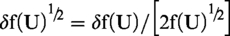
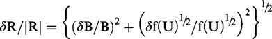
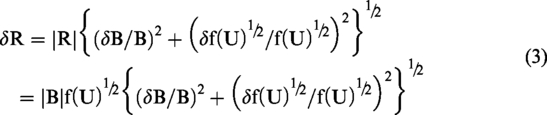
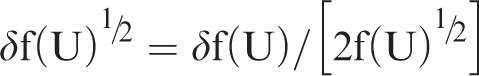
Unfortunately, upper and lower CI limits cannot be simply back-transformed as described in the previous paragraph. Uncertainty in the back-transformation factor must be taken into account. The estimated bias value (B) is uncorrelated with f(U)^½, and therefore after back-transformation to original scale values (R), the error relationship is given by the standard formula

$$\delta \text{R}/\left|\text{R}\right|={\left\{{\left(\delta \text{B}/\text{B}\right)}^{\text{2}}+{\left(\delta \text{f}{\left(\text{U}\right)}^{\mathrm{½}}/\text{f}{\left(\text{U}\right)}^{\mathrm{½}}\right)}^{\text{2}}\right\}}^{\mathrm{½}}$$

where δR, δB and δf(U)^½ are the uncertainties of the back-transformed bias, untransformed bias and predicted SD, respectively. Uncertainties in this context are usually expressed as SDs or as standard errors, but since CIs are constructed as coefficient x uncertainty, where coefficient is (usually) a critical value of Student’s t distribution, the error relationship could also be phrased in terms of CIs, i.e.

$$\begin{array}{l}\delta \text{R}=\left|\text{R}\right|{\left\{{\left(\delta \text{B}/\text{B}\right)}^{\text{2}}+{\left(\delta \text{f}{\left(\text{U}\right)}^{\mathrm{½}}/\text{f}{\left(\text{U}\right)}^{\mathrm{½}}\right)}^{\text{2}}\right\}}^{\mathrm{½}}\\ \hspace{1em}=\left|\text{B}\right|\text{f}{\left(\text{U}\right)}^{\mathrm{½}}{\left\{{\left(\delta \text{B}/\text{B}\right)}^{\text{2}}+{\left(\delta \text{f}{\left(\text{U}\right)}^{\mathrm{½}}/\text{f}{\left(\text{U}\right)}^{\mathrm{½}}\right)}^{\text{2}}\right\}}^{\mathrm{½}}\end{array}$$

(3)

where δR, δB and δf(U)^½ are (95%) CIs. δB is immediately available as per the first paragraph of the Introduction section. The computer program ¹¹ optionally outputs values necessary to calculate a 95% CI for any predicted variance, δf(U), and this translates to δf(U)^½ via

$$\delta \text{f}{\left(\text{U}\right)}^{\mathrm{½}}=\delta \text{f}\left(\text{U}\right)/\left[\text{2f}{\left(\text{U}\right)}^{\mathrm{½}}\right]$$

Superficially it might appear that after back-transforming bias as a percentage value (P), errors would be described by

$$\begin{array}{l}\delta \text{P}=\left|\text{P}\right|{\left\{{\left(\delta \text{B}/\text{B}\right)}^{\text{2}}+{\left(\delta \text{f}{\left(\text{U}\right)}^{\mathrm{½}}/\text{f}{\left(\text{U}\right)}^{\mathrm{½}}\right)}^{\text{2}}+{\left(\delta \text{U}/\text{U}\right)}^{\text{2}}\right\}}^{\mathrm{½}}\\ =\text{1}00\left|\text{B}\right|\text{f}{\left(\text{U}\right)}^{\mathrm{½}}/\text{U}\{{\left(\delta \text{B}/\text{B}\right)}^{\text{2}}\\ {+{\left(\delta \text{f}{\left(\text{U}\right)}^{\mathrm{½}}/\text{f}{\left(\text{U}\right)}^{\mathrm{½}}\right)}^{\text{2}}+{\left(\delta \text{U}/\text{U}\right)}^{\text{2}}\}}^{\mathrm{½}}\end{array}$$

(4)

where δU is the 95% CI for U. Denoting the variances of the two methods under consideration as σ_A² and σ_B², f(U) estimates σ_A² + σ_B², i.e. the variance of pair differences. Since the expected variance of the pair means is (σ_A² + σ_B²)/4, δU is well approximated by tf(U)^½/2, where t is the 0.05 Student’s t value with (N–p) degrees-of-freedom and p is the number of variance function parameters. Unfortunately, equation (4) is incomplete because it does not account for the correlation between f(U) and U. Moreover, extensive simulations confirmed that the degree of correlation depends on the nature of the relationship between f(U) an U (i.e. the form of the variance function) and also shows marked variability across any particular range of U values (low correlation where variance function slope is small, typically near the assay detection limit, and larger at higher variance function slopes). Equation (3) is exact but equation (4) slightly overestimates back-transformed CI size. For practical purposes, it is probably the best approximation that can be obtained.

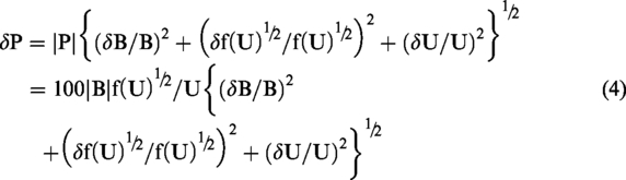
Equations (3) and (4) describe back-transformed CIs for bias. As per the first paragraph of the Introduction section, CIs for limits of agreement are related those for bias by the factor √3, and therefore back-transformed CIs for limits of agreement are √3δR and √3δP. Finally, when estimated bias is zero equations (3) and (4) reduce to

$$\delta \text{R}=\delta \text{Bf}{\left(\text{U}\right)}^{\mathrm{½}}$$

(5)

$$\delta \text{P}=\text{1}00\delta \text{Bf}{\left(\text{U}\right)}^{\mathrm{½}}/\text{U}$$

(6)

i.e. when bias is zero, CIs are back-transformed by the same simple factors that are applied to the bias and limits of agreement values themselves, and equation (4) inaccuracies vanish.

Results

The inset of Figure 1 shows the variance function (equation (2)) estimated from the 125 randomly drawn duplicates (β₁ = 0.01588, β₂ = 0.04397 and J = 2.83). The estimated 95% CI (δf(U)) is plotted as a shaded area. The data spanned more than eight orders of magnitude and a logarithmic scale on the ordinate is necessary to properly visualize the entirety of the variance function. The associated vertical stretching produces a somewhat distorted view of the fit to the data, and the CI, symmetrical about the variance function on a linear scale, appears asymmetric. The Figure 1 base graph shows the function replotted in terms of CV. For comparison, the estimated equation (1) (β₁ = 0.00000914, β₂ = 0.000769) is also plotted. Equation (1) was successfully used by Hawkins^5,6 to normalize paired oestradiol data. In general, it is likely to be an important normalizing function, but it cannot produce the U-shape necessary to provide for the upturn in CV often observed at the upper end of immunoassay measurement ranges.

Figure 1.

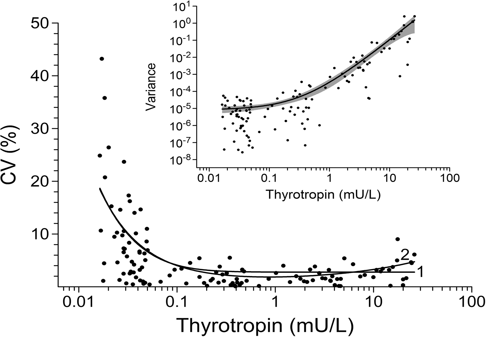
The inset shows the variance function, f(U) = (β₁ + β₂U)^J, estimated from 125 randomly drawn paired thyrotropin results. The shaded area is the 95% CI. The base graph shows the function replotted as CV (labelled 2) together with the estimated variance function, f(U) = β₁ + β₂U² (labelled 1).

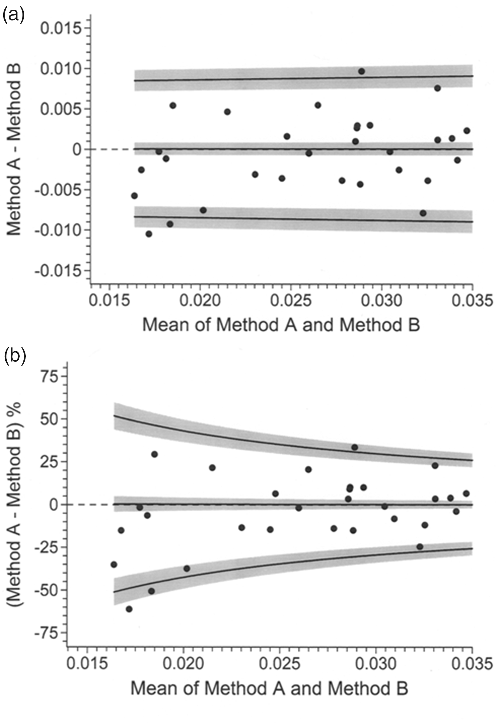
Figure 2 illustrates the paired results following Bland–Altman analysis (the first and second members of each (X, Y) pair were designated Method B and Method A, respectively). 95% CIs are plotted as shaded areas. Panels (a) and (b) give a clear illustration of the issue. The scatter of raw pair differences (Panel (a)) increases by orders of magnitude across the range of mean values, and consequently the calculated limits of agreement are a nonsensical reflection of the level of agreement between the paired results. The transformation 100d _i /U _i (Panel (b)) produced a marked improvement (an identical pattern of results could have been obtained by Bland and Altman’s logarithmic transformation). Nevertheless, it is unclear what the Panel (b) limits of agreement actually mean. In theory, they are limits which enclose ∼95% of pair differences and are intended to assist in determining whether the agreement between the two methods meets local clinical requirements. However, the limits in Panel (b) appear too narrow at the low end of the data range and are clearly far too wide elsewhere. In short, they are not fit for purpose. Although these are artificial data, the error properties are typical of numerous immunoassays (in particular) where clinically important results are located in regions where CV is simply not constant (i.e. logarithmic and 100d _i /U _i transformations fail). Panel (c) shows the result of transformation as d _i /f(U)^½. Breusch-Pagan statistics for Panels (a), (b) and (c) were 543.7 (P < 0.0001), 9.55 (P = 0.002) and 0.00085 (P = 0.977), respectively.

Figure 2.

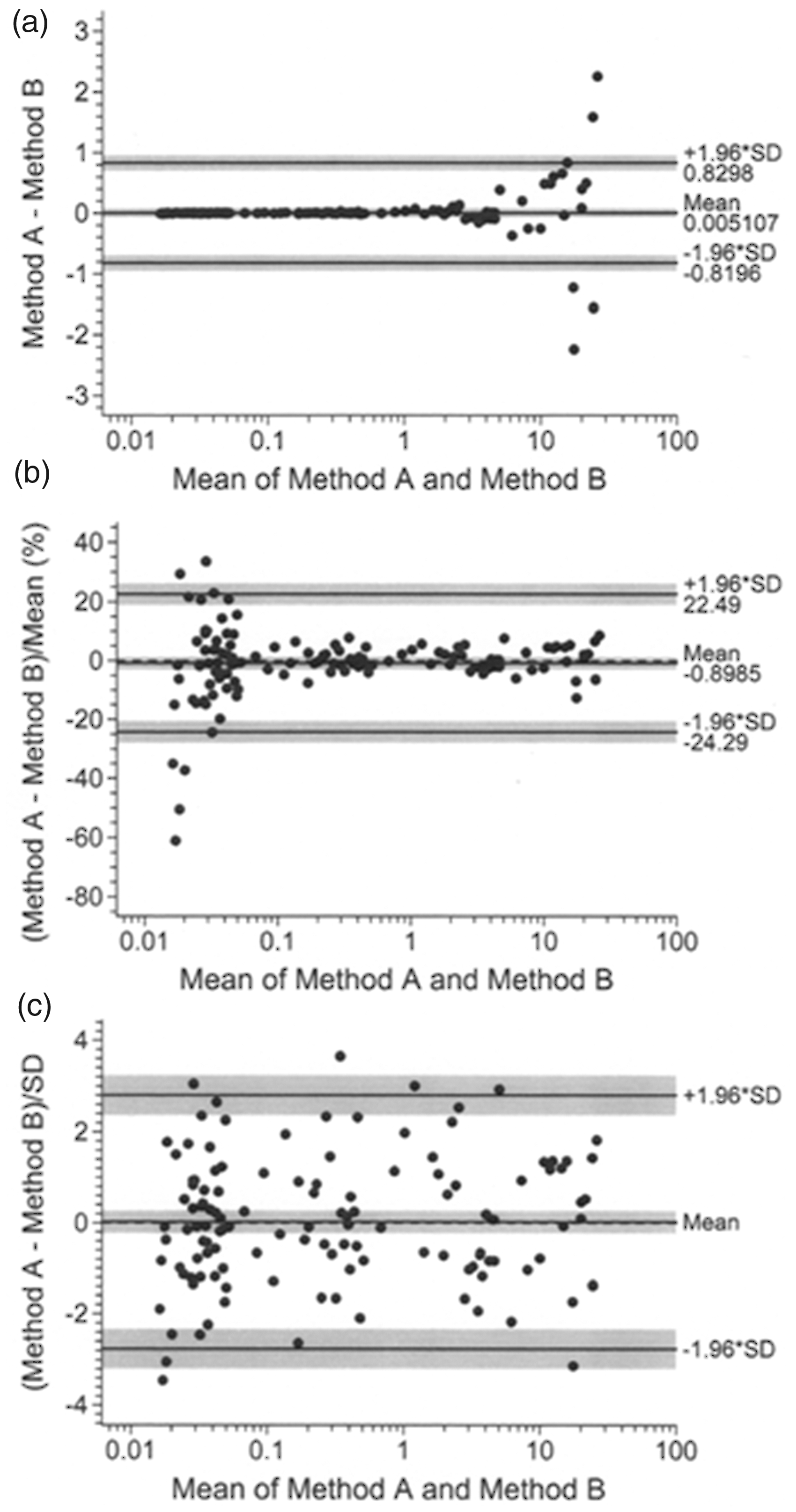
Bland–Altman analysis applied to the 125 randomly drawn thyrotropin pairs; raw pair differences d _i (a), differences transformed as 100d _i /U _i (b) and differences transformed as d _i /f(U)^½ (c) where f(U) was equation (2). Shaded areas are 95% CIs. Measurement units are mU/L.

Figure 3 illustrates the data points and bias and limits of agreement values, back-transformed from Figure 2(c), expressed in the original measurement scale (Panel (a)) and as percentages of the mean (Panel (b)). As expected, the data are identical to those in corresponding panels of Figure 2. Figure 3(a) is clearly useless as a visual aid and in general ‘blow-up’ views would be desirable. As an example, Figure 4 is a blow-up of the lower extreme of the data range. Transformation by variance function, as per Figure 2(c), has clearly produced a homogeneous scatter of pair differences across the entirely of the mean value range and therefore meaningful limits of agreement as envisaged by Bland and Altman. Graphs such as Figures 3 and 4 provide interpretation.

Figure 3.

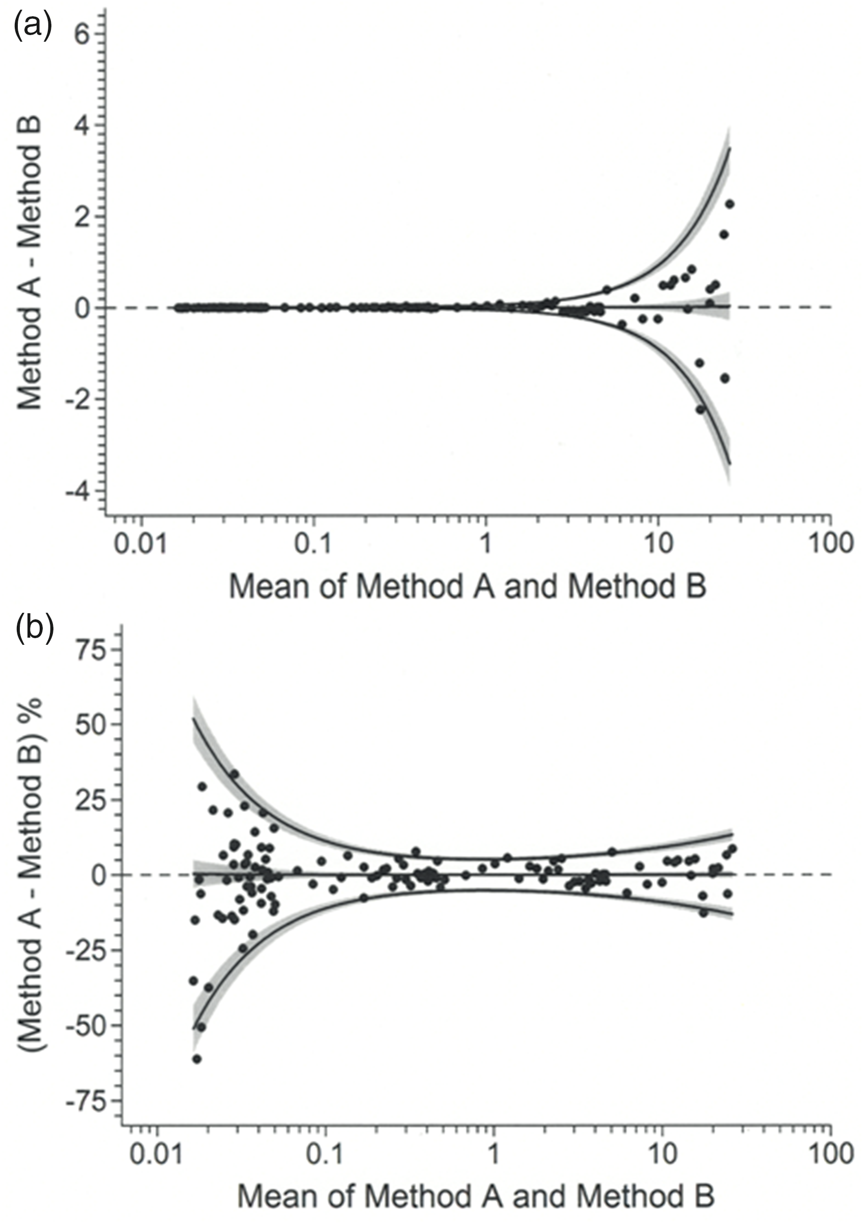
Data and results from Figure 2(c) back-transformed to the original measurement scale (a) and expressed as percentages of mean values (b). Measurement units are mU/L.

Figure 4.

Blow-up view of the lower extreme of the Figure 3 data range.

Equations (5) and (6) indicate that back-transformed CIs retain their exact relative size when bias is zero. It follows that when bias is very small relative to its CI, as is the case in Figure 2(c), then δB/|B| is large and completely dominates the other terms inside the curly brackets in equations (3) and (4). In other words, only a miniscule inflation in back-transformed CI size is expected in this particular case. Conversely, when B is large and particularly when δB/|B| < 1 (which equates to statistically significant bias), a marked increase in back-transformed CI size can be expected and examples of that are shown in the supplementary file.

Discussion

Simplicity and a highly informative graphical display are almost certainly the principal reasons for the popularity of Bland–Altman analysis. Results (horizontal lines) and an effective visual impression of uncertainty (CIs) are available at a glance. Bland and Altman ¹ warned against using any data transformation other than logarithmic because, as they rightly pointed out, the resulting bias and limits of agreement values would have no meaningful interpretation (hence those values are omitted from Figure 2(c)). However, Figure 2(a) and (b) illustrates the potential consequences of strictly adhering to Bland and Altman’s advice. Many real data-sets show similar behaviour and examples in the peer-reviewed literature are not difficult to find. ¹² The variance function can extend Bland–Altman analysis to encompass otherwise problematic data. Updating calculation and graphical software routines should present no great difficulties, but an additional interactive component would be required to allow users to enter or dial-up mean values of clinical interest, plus a display area to output the corresponding back-transformed bias and limits of agreement values.

Some might complain that the back-transformations illustrated in Figures 3 and 4 destroy the inherent straight-line simplicity of Bland–Altman plots. That is a valid point, but the immediate counter-argument is that simplicity equates, in some cases, to misleading or even meaningless results (particularly limits of agreement). There is no reason why curvilinearity should be especially disconcerting. Results from immunoassays are probably the most likely to require the calculations illustrated in Figures 3 and 4. In the 60 years since the method was discovered, immunoassay results, probably numbering in the trillions, have been routinely obtained by interpolating response measurements across curvilinear calibration relationships (standard curves). Estimating bias and limits of agreement by interpolation across curvilinear relationships should be regarded, at least by immunoassay practitioners, as just business as usual. The profiles in the main part of Figure 1 are not imprecision profiles (based instead on between-method differences), but the shape of the profile labelled 2 is readily identified as being characteristic of immunoassays. It is therefore worth comparing that familiar shape with the upper limit of agreement in Figure 3(b). The similarity is not a coincidence. In general, the shape of the normalizing variance function, plotted in terms of percent CV, predicts the shape of the agreement limits back-transformed as percentages. Similarly, the variance function in the inset of Figure 1, replotted as SD versus mean on a linear SD scale, predicts the shape of the agreement limits in Figure 3(a).

When conducting Bland–Altman analysis along traditional lines (Figure 2(a) and (b)), it is usually obvious, by simple visual inspection, which of the two configurations provides the more suitable data. Likewise, formal evaluation of the Figure 2(c) data is unnecessary because improved normalization is clearly obvious by eye (entirely expected in this case because the pair differences and variance function were highly correlated, by definition). However, in general, real data may require experimentation to determine which variance function provides the best normalization and this can be established objectively by comparing Breusch-Pagan P-values (Hawkins’ adaption of the test arguably has its greatest value in this particular context). Alternatively, the test can be used to simply ascertain whether normalization has been successful at some level of statistical significance (the small simulation reported in the Methods section suggests that the test is unlikely to produce seriously misleading P-values with typical Bland–Altman sample sizes). The supplementary file contains several examples which illustrate these considerations.

The computer program ¹¹ used to estimate equations (1) and (2) has been updated to perform the Bland–Altman calculations and graphical output shown here. The program incorporates several variance functions any of which can be evaluated as a normalizing function.

Supplemental Material

Supplemental material for Using the variance function to generalize Bland–Altman analysis

Supplemental material for Using the variance function to generalize Bland–Altman analysis by William A Sadler in Annals of Clinical Biochemistry